Microbiome dynamics during the HI-SEAS IV mission, and implications for future crewed missions beyond Earth
←
→
Page content transcription
If your browser does not render page correctly, please read the page content below
Mahnert et al. Microbiome       (2021) 9:27
https://doi.org/10.1186/s40168-020-00959-x

 RESEARCH                                                                                                                                          Open Access

Microbiome dynamics during the HI-SEAS
IV mission, and implications for future
crewed missions beyond Earth
Alexander Mahnert1, Cyprien Verseux2, Petra Schwendner3, Kaisa Koskinen1,4, Christina Kumpitsch1, Marcus Blohs1,
Lisa Wink1, Daniela Brunner1, Theodora Goessler1, Daniela Billi5 and Christine Moissl-Eichinger1,4*

  Abstract
  Background: Human health is closely interconnected with its microbiome. Resilient microbiomes in, on, and around the
  human body will be key for safe and successful long-term space travel. However, longitudinal dynamics of microbiomes
  inside confined built environments are still poorly understood. Herein, we used the Hawaii Space Exploration Analog and
  Simulation IV (HI-SEAS IV) mission, a 1 year-long isolation study, to investigate microbial transfer between crew and habitat, in
  order to understand adverse developments which may occur in a future outpost on the Moon or Mars.
  Results: Longitudinal 16S rRNA gene profiles, as well as quantitative observations, revealed significant differences
  in microbial diversity, abundance, and composition between samples of the built environment and its crew. The
  microbiome composition and diversity associated with abiotic surfaces was found to be rather stable, whereas
  the microbial skin profiles of individual crew members were highly dynamic, resulting in an increased
  microbiome diversity at the end of the isolation period. The skin microbiome dynamics were especially
  pronounced by a regular transfer of the indicator species Methanobrevibacter between crew members within the
  first 200 days. Quantitative information was used to track the propagation of antimicrobial resistance in the
  habitat. Together with functional and phenotypic predictions, quantitative and qualitative data supported the
  observation of a delayed longitudinal microbial homogenization between crew and habitat surfaces which was
  mainly caused by a malfunctioning sanitary facility.
  Conclusions: This study highlights main routes of microbial transfer, interaction of the crew, and origins of
  microbial dynamics in an isolated environment. We identify key targets of microbial monitoring, and emphasize
  the need for defined baselines of microbiome diversity and abundance on surfaces and crew skin. Targeted
  manipulation to counteract adverse developments of the microbiome could be a highly important strategy to
  ensure safety during future space endeavors.
  Keywords: Confined built environments, Isolation, HI-SEAS, Skin microbiome, Indoor microbiome, 16S rRNA gene
  amplicons, qPCR, Antimicrobial resistances, Longitudinal, Phenotype predictions

* Correspondence: christine.moissl-eichinger@medunigraz.at
1
 Interactive Microbiome Research, Diagnostic & Research Institute of
Hygiene, Microbiology and Environmental Medicine, Medical University of
Graz, Neue Stiftingtalstrasse 6, 8010 Graz, Austria
4
 BioTechMed-Graz, Graz, Austria
Full list of author information is available at the end of the article

                                       © The Author(s). 2021 Open Access This article is licensed under a Creative Commons Attribution 4.0 International License,
                                       which permits use, sharing, adaptation, distribution and reproduction in any medium or format, as long as you give
                                       appropriate credit to the original author(s) and the source, provide a link to the Creative Commons licence, and indicate if
                                       changes were made. The images or other third party material in this article are included in the article's Creative Commons
                                       licence, unless indicated otherwise in a credit line to the material. If material is not included in the article's Creative Commons
                                       licence and your intended use is not permitted by statutory regulation or exceeds the permitted use, you will need to obtain
                                       permission directly from the copyright holder. To view a copy of this licence, visit http://creativecommons.org/licenses/by/4.0/.
                                       The Creative Commons Public Domain Dedication waiver (http://creativecommons.org/publicdomain/zero/1.0/) applies to the
                                       data made available in this article, unless otherwise stated in a credit line to the data.
Mahnert et al. Microbiome (2021) 9:27 Page 2 of 21 Background productivity may be a significant loss given the high This decade may see the beginning of a sustainable hu- value of astronaut working time. man presence on the Moon. The US government stated Another threat comes from microorganisms’ interfer- their commitment to lead such an endeavor in the Space ence with equipment. First, some microorganisms, re- Policy Directive-1 [1] and current goals include landing ferred to as technophiles, can colonize industrial a crew at the Moon’s south pole by 2024, before estab- materials and lead to hardware malfunction, degradation lishing a sustained presence there by 2028 [2]. Since of structural materials, and corrosion of metal parts [21]. 2015, the European Space Agency (ESA) has been Technophiles were found onboard the Mir station [22, strongly advocating its “Moon Village” concept, a large 23] and onboard the ISS [13, 19, 24], leading to damage collaborative undertaking that would lead to a perman- of various systems [25, 26]. Second, microbial contami- ent presence on the Moon [3]. In addition, the latest nants could interfere with biological life-support systems Council at ministerial level anticipates a strong involve- [27]. These life-support systems could greatly contribute ment of ESA in the US-led Moon program [4]. Other to the feasibility of long-term missions on the Moon or collaborators include the Japan Aerospace Exploration Mars [28–30]. However, microbial contaminants could Agency (JAXA) and the Canadian Space Agency (CSA). harm the system-relevant organisms through competi- While lunar exploration could greatly benefit different tion and/or toxicity or by making food products unsuit- areas of science and technology in itself [5, 6], the Moon able for crew consumption. is expected to serve as a testing ground for crewed mis- Finally, microorganisms brought alongside the crew sions to Mars. Reaching the red planet is also the stated could interfere with the search for life on Mars [31, 32]. goal of private spacecraft companies, notably SpaceX [7] One strategy to mitigate the risk of contamination could who aims for a landing as early as in the 2020s. be to increase our knowledge of, and to catalogue, the In such endeavors, microorganisms will inevitably co- microbial communities we are carrying [33, 34]: this travel with the crew: they are thought to outnumber hu- would help to discriminate between endogenous life and man cells in our bodies [8] and each individual releases our microbiome in case of an ambiguous discovery and millions of them every hour [9]. A microbe-free crewed to assess the risk of contaminants to adapt to some local mission is unrealistic, unethical, and undesirable, as our (micro)environments. While Mars’s surface appears hos- microbiome is essential to our health [10]. Microbial tile even to microbial life, it cannot be excluded that communities may however pose, if inadequately man- some extremophiles may reach niches where they could aged, serious threats to future missions. remain active [32]. The most obvious threats to the crew’s health are In any case, microbial communities will be critical pathogens. This risk is exacerbated by crew members’ components of future space endeavors, with a potentially confinement and proximity, limited treatment options, large influence on mission success [35]. Their import- increased microbial transmission in microgravity [11], ance is reflected in space agencies’ efforts to characterize restricted hygienic practices, potentially increased them onboard the ISS [13, 19, 24, 36–40]. virulence and decreased antibiotic susceptibility of However, microbial monitoring on the ISS is con- bacteria in space [11–14], and lowered immune re- strained by logistical and funding challenges. An alterna- sponses of astronauts attributed to microgravity, radi- tive is to study microbiome nature and dynamics in ation, and stress [11, 12, 15–17]. Moreover, the lack similar, closed systems (such as submarines and polar of environmental microorganisms competing with stations) or specific, ground-based analogues of long- human-borne pathogens for the same niche could term crewed spaceflight [18, 41]. While those analogues complicate the establishment of resilient microbiomes differ in some important aspects (e.g., gravity and radi- in their habitat [18]. While no life-threatening infec- ation) from spaceflight itself, they place a small, isolated tions have been reported during spaceflight so far, op- crew in combinations of the following: long-term con- portunistic pathogens, which are part of the normal finement, high workloads, restricted waste disposal, lim- human-associated microbial diversity, were detected ited hygiene, and/or low air or water quality. They offer on the International Space Station (ISS) [13, 19]. Such the possibility to comprehensively monitor related pathogens might have caused tens of minor medical medical and psychological issues. incidents—among which are urinary tract, upper re- In the past, several studies on the indoor and human spiratory tract and subcutaneous skin infections—be- microbiome were conducted in settings simulating mis- yond Earth [11, 16]. sions to future facilities on the Moon or Mars, for in- The threat increases when emergency returns become stance: Mars500 (520 days) [41, 42], the Antarctic base impossible, notably on a Mars journey, which is ex- Concordia (1 year) [43], the inflatable lunar/Mars analo- pected to last at least 520 days [20]. Even in a relatively gous habitat (ILMAH) (30 days) [44], and the biological mild disease scenario, the resulting decrease in life-support testbed “Lunar Palace 1” (LP1; 105 days)
Mahnert et al. Microbiome   (2021) 9:27                                                                    Page 3 of 21

[27]. For all these studies, individual parameters have to   washed with Equate’s Sensitive Skin Body Wash, and
be critically considered such as variations in methodolo-    hair with Garnier Fructis’ Pure Clean Clear 2in1. In-
gies, environmental conditions, activity, geographical lo-   between showers, participants occasionally used disin-
cation, architectural design, baseline-diversity of          fecting wipes (mainly, Kirkland’s Extra Large Disinfect-
microorganisms, contaminants from crew members, and          ing Wipes). Hands were routinely washed with Dr.
cargo such as food and scientific equipment.                 Bronner’s 18-in-1 Hemp Peppermint Pure-Castile liquid
  Another opportunity arose in 2015–2016: as part of         soap, and disinfected with germ’s hand sanitizer.
the Hawaii Space Exploration Analog and Simulation IV          A general cleaning of the habitat was performed every
(HI-SEAS IV) mission, six people spent 1 year in isola-      Sunday. Most hard surfaces were then cleaned with Sim-
tion in a dome (diameter: 11 m) located at 2.5 km of         ple Green’s cleaner, the kitchen floor with Comet’s
altitude on the barren slopes of the Mauna Loa volcano,      bleach-based powder, and floors aside from the bath-
primarily for NASA Behavioral Health and Performance         room and kitchen were only vacuumed. Dishwashing
(BHP) research [45]. Over a period of 336 days, swab         was performed by hand. Clothes were washed with Kirk-
and wipe samples from habitat surfaces and crew skin         land’s UltraClean laundry detergent, either by hand or in
were taken in order to assess the microbial community        a washing machine.
fluctuation, as well as the interactions of surface and        Sources of voluntarily introduced microorganisms in-
skin microbiomes.                                            cluded the following: Fermented products (sourdough
  Our main hypotheses were that (i) the microbiome of        bread, tempeh, cream cheese, kombucha, and yoghurt)
the HI-SEAS habitat would follow a longitudinal              were prepared using commercial microbial mixes. Toi-
homogenization between individual crew members, but          lets were composting toilets, maintained with Sun-Mar’s
also the surrounding built environment; (ii) overall mi-     Microbe Mix and Sun-Mar’s compost swift. Cyanobac-
crobial diversity would be depleted; and (iii) the micro-    teria (Anabaena sp. PCC 7120 and Chroococcidiopsis sp.
biome would resemble those of other long time                CCMEE 029) were used for research purposes. Part of
experiments in isolated and confined built environments      the kitchen waste was processed in a bokashi compost-
(ICE) on Earth and on the ISS.                               ing system (purchased from Each One Teach One
                                                             Farms, Hawaii).
Methods
Setting of the HI-SEAS IV mission                            Sampling
The 1-year Hawaii Space Exploration Analog and Simu-         Microbiome samples were taken every other week. Habi-
lation IV (HI-SEAS IV) mission took place from August        tat/furniture surface samples were taken with swabs at
28th, 2015 to August 28th, 2016 [45] in the HI-SEAS          four different locations. Skin surface (front torso) sam-
habitat, an 11 m in diameter spherical-shaped dome lo-       ples were taken with wipes from each crew member. In-
cated at 2.5 km of altitude on the barren slopes of the      mission sampling occurred from September 4th, 2015 to
Mauna Loa volcano (Supplementary Fig. S1). Operated          August 5th, 2016, and an extra series of skin wipe sam-
by the University of Hawaii, and funded by NASA, this        ples was performed after mission completion. The base-
habitat served primarily for NASA Behavioral Health          line (day 0) was defined as the day of the first sampling
and Performance (BHP) research. During HI-SEAS IV,           event.
six crew members (3 males and 3 females) selected for           The swab samples were taken from (Supplementary
their astronaut-like profile, four from the USA and two      Fig. S2):
from Europe (France and Germany), spent a year there
in conditions mimicking those of a Mars mission. Time         – The front part of the (composting) toilet bowl (high
was mostly spent on research work (including outside            density plastic), in the upstairs bathroom
work, wearing mock spacesuits), test subject duties,          – The kitchen floor (painted, waterproof plywood), in
physical exercise, and household chores. The crew was           an area (between the fridge and another piece of
physically isolated from other human beings for the             furniture) where dust tended to accumulate
whole mission duration and communications had a high          – The desk (medium density fiberboard overlaid with
latency (20-min delay in both directions). The diet was         plastic laminate) in one of the bedrooms, and
mostly composed of dehydrated food, canned food,              – One desk (medium density fiberboard overlaid with
occasional fermented food (yoghurt, bread, and cream            plastic laminate) in the main room
cheese) made from rehydrated products, and rare vege-
tables grown on site.                                          For each habitat/furniture surface sample, a swab
  Participants typically showered 1 to 3 times a week,       (552C regular swab; ethylene oxide sterilized, Copan,
for an average duration of 1.5 to 2 minutes under run-       Brescia, Italy) was moistened with autoclaved, deionized
ning water (Heinicke et al. submitted); bodies were then     water (ELGA’s Vision 125 Deionizer). An area of 5 × 5
Mahnert et al. Microbiome (2021) 9:27 Page 4 of 21
cm was sampled in three directions (horizontal, vertical, followed by 35 cycles of denaturation at 94 °C for 45 s,
and diagonal). The swab was turned between each annealing at 50 °C for 60 s, elongation at 72 °C for 90 s,
change in direction. The swab was then broken at the and a final elongation step at 72 °C for 10 min. PCR
predetermined breaking point and placed back into its fragments were evaluated for product size and quantity
original container. Field controls were performed during by agarose gel (3%) electrophoresis at 70 V for 30 min.
each sampling session by waving the swab in the air for Libraries for Illumina MiSeq sequencing were prepared
a few seconds instead of sampling a surface. by the Core Facility Molecular Biology at the Center for
Prior to samplings of skin surfaces, sterile 50-ml tubes Medical Research at the Medical University Graz,
were filled with one wipe (TX3211, SterileWipe LP, Tex- Austria and covered biological samples, field blanks, ex-
wipe) and 10 ml of autoclaved, deionized water. Once traction blanks, as well as no-template controls of PCRs.
the wipes were homogeneously moistened, crew mem- For the NGS library, DNA concentrations of the gener-
bers sampled their own skin following oral and written ated amplicons were normalized with a SequalPrep™
instructions. Briefly, they put on gloves, cleaned them normalization plate (Invitrogen). After normalization of
with ethanol, took the wipe out of the tube, put it flat on PCR products, each sample was indexed with a unique
their hand, wiped their torso up and down and left and barcode sequence using 8 cycles of indexing PCR.
right, folded the wipe over the target surface, wiped Indexed samples were then pooled and purified by gel
again with one of the clean sides, wiped with the other cuts. Finally, the library was sequenced on an Illumina
side, and put the wipe back into the original tube. MiSeq instrument and the MiSeq Reagent Kit v3, 602
Twenty milliliters of water were then added to each tube cycles (2 × 301 cycles).
before storage. Field controls were performed during
each sampling session by waving the wipe in the air for Statistics and bioinformatics
a few seconds instead of wiping skin. After sequencing, resulting fastq files were processed with
Swab and wipe samples were stored at − 20 °C after Qiime2 versions 2018.6–2020.8 [47]. Demultiplexed reads
sampling, shipped to Europe in dry ice after mission were denoised with DADA2 [48] and an amplicon se-
completion and then stored at − 80 °C until analysis. quence variant (ASV) feature table was created after trun-
cating forward reads at position 200 and reverse reads at
DNA extraction position 150. Potential contaminants were identified and
A total of 63 wipes were thawed at 4 °C overnight before removed with decontam [49] and its prevalence method
transferring them to DNA-free bottles (baked at 250 °C with default settings (method = “prevalence,” neg=“is.neg,”
for 24 h) filled with polymerase chain reaction (PCR)- threshold = 0.5). Representative sequences were classified
grade water. The bottles were sonicated for 120 ± 5 s by a Naïve Bayes trained classifier [50] based on Silva 128
with a maximal power of 240 W and a frequency of 40 [51, 52] and a rooted phylogenetic tree for phylogenetic
kHz, and vortexed at maximum speed for 1 min. The diversity measures was created with Fasttree [53]. Core
biomass-containing water suspension was concentrated metrics for alpha and beta diversity (including metrics for
to 200–500 μl using UV sterilized Amicon filters (Ami- richness, evenness, diversity, and distances) were calcu-
con Ultra 15 ml, 50 K, Merck Millipore). lated including phylogenetic measures like UniFrac [54] at
DNA was then extracted from cells suspended and a depth of 3000 sequences per sample. Diversity analysis
concentrated from wipes, and from all surface swabs covered displays and statistics like rarefaction curves, prin-
plus 7 swab field controls (for a total of 111 swab cipal coordinate analysis (PCoA), procrustes analysis,
samples), using QIAGEN’s DNeasy PowerSoil Kit. biplots, Mantel tests [55], Kruskal-Wallis, bioenv [56],
Spearman rank correlations [57], Adonis (conducted in
16S rRNA gene amplicons Qiime 1.9.1), ANOSIM, or PERMANOVA tests. Meta-
Microbial profiles were based on amplicons targeting the analysis of longitudinal microbial diversity inside built en-
V4 region of the 16S rRNA gene. The common primer vironments was conducted in Qiita [58] and used datasets
pair F515-R806 [46] with tags for Illumina sequencing of the following publicly available Qiita studies: 2192,
was used to cover most bacterial and some archaeal taxa 10423, 11740, and 12858. All selected studies (including
(Supplementary Table S1). Twenty-five microliters of our study as well) targeted the V4 region of the 16S rRNA
the PCR reaction mix contained a final concentration of gene and were processed with the very same Qiita stand-
200 mM each of forward and reverse primer (0.4 μl of ard workflows (trimmed to 150 bp, used Deblur for
10 μM stock each), 0.1 μl TaKaRa ExTaq polymerase (5 denoising of the ASVs and Greengenes 13_8 for closed
U/μl, Clontech, Japan), 2 μl ExTaq buffer with MgCl2 reference taxonomy assignments). Longitudinal analysis
(10×), 1.6 μl dNTP mix (2.5 mM), 2 μl of template was based on the q2-longitudinal plugin available in
DNA, and 18.5 μl PCR grade water. PCR conditions Qiime2 [59] and covered calculations of feature-volatility,
were as follows: initial denaturation at 94 °C for 3 min, linear-mixed-effects modeling, pairwise-differences,Mahnert et al. Microbiome (2021) 9:27 Page 5 of 21
pairwise-distances, Wilcoxon signed rank tests, and above 0.9 as well as clean melting curves were required.
Mann-Whitney U tests. Supervised classification and re- Counts in negative and no-template controls were sub-
gression of sample metadata was conducted with the q2- tracted from actual samples and extrapolated per m2.
sample-classifier plugin [60] with settings for optimized Finally, qPCR counts were displayed as volatility plots
feature-selection and parameter tuning for RandomForest including linear regressions with time.
regression and classifications. For this analysis, the dataset In addition to quantifications of the microbial load,
was randomly split and 20% of the dataset was removed monitoring of antimicrobial resistances was based on the
and kept as the test set. The training set was used to cre- following four selected resistance genes: blaOXA (class
ate a learning model predicting class probabilities for each A beta-lactamase [74];), int1a (class 1 integrase [75]),
sample by using K-fold cross validation. In the end model, qacEΔ1 (biocide resistance gene, quaternary ammonium
accuracy was calculated by comparing predicted values of compound-resistance [74, 76]), and tetM (tetracycline
the training and test set. Differential abundance and com- resistance [74, 77]) (Supplementary Table S3). As indi-
position of features was determined with balances in vidual standards were not available, all quantifications
gneiss [61], ancom [62], and feature rankings (feature dif- were based on relative proportions and serial dilutions
ferentials and loadings) available from aldex2 [63], song- (1:10, 1:100, 1:1,000) of the genomic DNA of four cul-
bird [64], and deicode [65] were partly visualized in qurro tures (Acinetobacter sp., Escherichia coli, Enterococcus,
[66]. Microbial contributions of different sources and and Pseudomonas aeruginosa) with reported presence of
sinks were predicted with SourceTracker2 (https://github. these resistances. qPCR runs were prepared with the
com/biota/sourcetracker2 [67]) at a source and sink depth STARlet pipetting robot (Hamilton, Germany) for the
of 3000 sequences per sample. Potential phenotypes and Bio-Rad CFX384 instrument. PCR conditions were set to
functions were predicted with PiCrust2 (https://github. initial denaturation at 95 °C for 10 min, followed by 40
com/gavinmdouglas/q2-picrust2 [68]) using the custom cycles of denaturation at 95 °C for 15 s, annealing at 55
tree pipeline and BugBase [69–71]. Further statistics and °C for 30 s, elongation at 72 °C for 30 s, and a final
visualizations were conducted in R [72] using the libraries elongation step at 72 °C for 30 s. All 14 qPCR runs were
ggplot2 and streamgraph. normalized internally (according to qPCR counts of each
individual standard); counts from negative controls and
Data availability no-template controls were subtracted from actual sam-
All amplicon raw data is available at the European Nu- ples and then extrapolated per m2. Similarly, as done for
cleotide Archive ENA (EMBL-EBI ERP118380). In qPCR counts of the 16S rRNA gene, antimicrobial resis-
addition to raw data, processed data is available in Qiita tances were also displayed as volatility plots with linear
(study id 12858; https://qiita.ucsd.edu/ [58]). regressions.
qPCR (16S rRNA genes and resistance genes) Microbial nomenclature
The overall microbial load was determined by qPCR of Throughout the manuscript, we refer to the nomencla-
the 16S rRNA gene. Two setups were used to quantify ture assigned by the Silva 128 release. A special case is
bacteria and archaea separately (primer pair 331f-797r the genus Propionibacterium. We are aware that skin-
for bacteria [73] and primer pair A806f-A958r for ar- associated representatives of this genus were renamed in
chaea, Supplementary Table S2). For each setup 10 μl of a recent release of the Silva database to the genus
the SYBR Green Supermix (Biorad) contained 5 μl of Cutibacterium [78] that was not available when we per-
SsoAdvanced Universal qPCR Kit MM 2×, 0.3 μl each of formed our analysis.
forward and reverse primers (10 μM), 3.4 μl of PCR-
grade water, and 1 μl of template DNA. qPCR runs were Results
then carried out on a Bio-Rad CFX96 thermocycler with Overview of the microbiome of the built environment
the following conditions: initial denaturation at 94 °C for and its occupants
3 min, followed by 35 cycles of denaturation at 94 °C for Samples were taken from four representative locations
45 s, annealing at 54 °C for bacteria, and 60 °C for ar- (toilet bowl, kitchen floor, desk in one of the bedrooms,
chaea for 60 s, elongation at 72 °C for 90 s, and a final desk in the main room) within the confined built envir-
elongation step at 72 °C for 10 min. Quantifications of onment and from the skin (front torso) of six isolated
16 qPCR runs relied on serial dilutions of a cloned 16S crew members. Sampling was performed at 27 time
rRNA gene of Escherichia coli and Nitrososphaera vien- points spanning 1 year. Besides amplicon sequencing, all
nensis, respectively for bacteria and archaea, into Strata- samples plus laboratory controls (n = 186 in total) were
Clone vector pscA_AmpKan according to manufacturer subjected to quantitative PCR (qPCR) on the 16S rRNA
instructions. For reliable quantifications, a minimum re- gene to assess the overall bacterial load, and on four rep-
action efficiency of 0.8 and a correlation coefficient resentative resistance genes (blaOXA, int1a, qacEΔ1,Mahnert et al. Microbiome (2021) 9:27 Page 6 of 21 tetM) to assess the progression of microbial resistances Since we were interested in the characteristics of the on skin and surfaces over time. microbiome profile of the different sample groups, the Along with the samples, 16 types of metadata of envir- dataset was divided into different surface types (crew onment and crew members were recorded (selected nu- [skin], built environment) and sample locations (e.g., in- merical metadata is listed in Supplementary Table S4). dividual crew members and locations within the facility). The crew was composed of three male and three female members (crewID A-F), with an average age of 30 ± 4 and The overall microbial diversity and composition of biotic an average body size of 176 ± 9 cm. During the isolation (skin) and abiotic surfaces differs significantly and confinement, hygiene practices were restricted. On In the first step, we compared the alpha diversities average, crew members showered preferentially on Satur- (based on Shannon index) of all sample types. Samples days, every 5.4 ± 1.8 days (60.67 ± 15.7 times) for about 1 from the crew’s skin showed significantly lower diversity min and 42 ± 47 s. However, individual showering prac- than samples from surfaces of the built environment tices differed. For instance, some crew members showered (pairwise Kruskal-Wallis P = 7.3 × 10⁻¹⁶; mean Shannon for shorter durations, but more frequently and others H’ ~ 6.2 vs. 7.5) (Fig. 1a). Significant differences were showered for longer durations, but only a few times dur- also detected in the diversity index of five crew members ing the isolation period. The diet was mostly composed of (pairwise Kruskal-Wallis of crew member A and B: q dehydrated food, but the crew was allowed to bring bene- value 1.6 × 10⁻³; A and D: q value 1.3 × 10⁻³; A and F: ficial microbes into the habitat, e.g., starters for sourdough 7.5 × 10⁻³; C and F: 2.7 × 10⁻²; Fig. 1c). bread, tempeh, cream cheese, kombucha, and yoghurt. Notably, the microbial diversity on the crew’s skin varied Toilets were composting toilets. Cyanobacteria (Anabaena more (mean Shannon H’ ~ 5.0 in samples from crew sp. PCC 7120 and Chroococcidiopsis sp. CCMEE 029) member F to ~ 6.7 for crew member A) than that on abi- were used for research purposes. Part of the kitchen waste otic surfaces (mean Shannon H’ ~ 7.2 in samples of the was processed in a bokashi composting system. kitchen floor to ~ 7.6 in bedroom samples; Fig. 1b, c). No direct or real-time contact to other humans except With respect to alpha diversity, the built environment to crew members was allowed, and the extravehicular surfaces showed only significant differences between activities included donning of a mock spacesuit that pre- bedroom and kitchen floor samples (pairwise Kruskal- vented exposure to open air and direct sunlight (de- Wallis q value 4.5 × 10⁻²; Fig. 1b), while richness was scribed in [79]). Nine resupply events happened during variable (Supplementary Fig. S3). Alpha diversity was the isolation period (on days 15, 43, 79, 107, 148, 185, also significantly different according to type of surface 223, 258, 303, 335). A total of 132 samples were proc- material (plywood vs. polymer; pairwise Kruskal-Wallis q essed before and 43 samples after a resupply event. value 4.5 × 10⁻²; Supplementary Fig. S4). Temperature was stable over time (mean temperature 18 Beyond alpha diversity, the microbiome profile of sam- ± 1 °C). CO2 levels were always in the recommended ples from built environment surfaces was significantly range for indoor environments (400–1000 ppm) with an different from that of crew skin samples (weighted Uni- average of 662 ± 62 ppm. Frac distances, PERMANOVA q value = 3 × 10⁻³; ANO- Denoising of demultiplexed amplicon data with DADA2 SIM R = 0.3, P = 3.3 × 10⁻³; Adonis R2 = 0.15, P = 1 × resulted in 10,016 unique features (ASVs). In an initial 10−3) and samples clustered separately in PCoA plot step, we analyzed the processed controls (sampling blanks, analysis (Fig. 1g, h). Further significant differences were process controls, no-template controls), which showed found between all four locations of the HI-SEAS habitat significantly lower microbial Shannon diversity than in ac- (ranging from q values of 1.8 × 10⁻³ to 3.3 × 10⁻³, tual samples (pairwise Kruskal-Wallis P = 1.8 × 10⁻⁴; PERMANOVA pairwise testing; ANOSIM R = 0.14 to Shannon H’ ~ 5.7 vs. 7.0; rarefaction depth of 7850 se- 0.85, highest for kitchen floor vs. toilet bowl; Adonis R2 quences). Moreover, microbial composition differed sig- = 0.33). However, the microbial composition was not nificantly between samples and controls, according to significantly different between individual crew members weighted UniFrac metrics (PERMANOVA, ANOSIM R = despite highly explained variability along PCoA axis 1, 0.42, Adonis R2 = 0.06, for all three tests P = 0.001). To indicating dynamic changes of microbial composition on clean the dataset, contaminants were identified from proc- skin samples over time (see below). essed controls with decontam [49] and subsequently re- Supported by extensive metadata analysis, the factors time moved from the dataset. All subsequent analyses were (P = 0.04, Spearman rank correlation of Shannon diversity performed with the cleaned dataset, which contained 3, with time) and sampling location (P = 9.4 × 10⁻¹⁹, Kruskal- 077,780 sequences (median frequency was 17,533 se- Wallis test of all groups, see above for more details) were quences per sample). According to rarefaction curves, se- identified to have a significant impact on microbial diversity quencing depth was of sufficient quality, as the Shannon and the microbial profile, whereas the microclimate of the diversity metric (H) plateaued at ~ 2500 sequences. habitat revealed no significant influence.
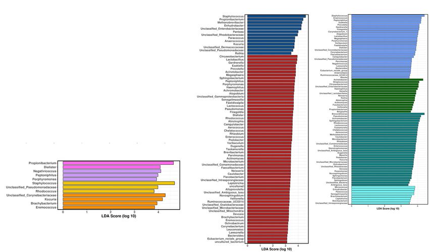
Mahnert et al. Microbiome       (2021) 9:27                                                                                            Page 7 of 21

 Fig. 1 Microbiome profile of crew and built environment samples, all time points included. a–c Violin plots (kernel probability density of Shannon
 values, displaying the alpha diversity) including individual data points and a box with median and interquartile range. a Sampled surface types:
 skin of crew and locations of the built environment. b Built environment surfaces: BR (desk in bedroom), KC (kitchen floor), MR (desk in main
 room), TB (toilet bowl). c Samples from the individual crew members (a–f). d Linear discriminant analysis effect size (LEfSe) on samples from crew
 and built environment. e LEfSe on samples from built environment surfaces. f LEfSe on samples from individual crew members. g–h Beta
 diversity represented by PCoA plots based on weighted UniFrac metrics and a rarefaction depth of 3000 ASVs per sample. g Microbial profile of
 samples from built environment and crew. h Microbial profile of the individual crew members and sampling locations of the built environment
Mahnert et al. Microbiome   (2021) 9:27                                                                       Page 8 of 21

   Metadata predictions based on Random Forest classi-       (Supplementary Fig. S6). An increase in microbial di-
fiers and regressors showed high overall accuracy esti-      versity on skin was observed for most crew members
mates of 95% for the sampling environment (skin samples      (C, D, E, and F; mean Shannon H′ 5.1 to 6.5; highest
vs. built environment samples), and the day of sampling      increase for individual C from 5 to 7.8). However,
(R = 0.77, P = 2.3 × 10⁻⁸). Thus, our subsequent analyses    almost no change was visible for individual A, and a
focused on the impacts of time and sampling location.        slight decrease was observed for individual B (mean
                                                             Shannon H′ 5.5. to 4.8; Fig. 2b).
Each surface was characterized by a specific set of             The microbial diversity on different locations inside
microbial signatures, which can be predicted with high       the HI-SEAS habitat changed as well (Fig. 2b). The lar-
accuracy                                                     gest fluctuations were detected for samples of the main
As selected surfaces of the built environment (desk in a     room, and a slight increase in microbial diversity was
bedroom, kitchen floor, desk in the main room, toilet        visible for all locations apart from the toilet bowl. In the
bowl) and the crew’s skin showed a significantly different   latter case, microbial diversity decreased by 1 log (mean
composition (see below), we were interested in a detailed    Shannon H′ 7.9 to 6.8), possibly due to more rigorous
analysis of the characteristic features.                     cleaning procedures.
   Overall, the skin samples were characterized by high         Other metrics describing the alpha diversity of all sam-
abundance of Staphylococcus, Propionibacterium, Entero-      ples, such as richness (92 to 213.67) and phylogenetic di-
bacteriaceae, Enhydrobacter, and Methanobrevibacter          versity estimates (7.6 to 14.7), followed a similar pattern,
signatures (LEfSe analysis, Fig. 1d), whereas the built      while Pielou’s evenness remained constant over the en-
surfaces were characterized by the presence of Chryseo-      tire isolation period (0.8 to 0.84; Supplementary Fig. S7
bacterium, Lactobacillus, Gardnerella, Prevotella, and       and Supplementary Fig. S8).
Acinetobacter.                                                  Temporary dynamics of microbial diversity were inves-
   Indicative microbial signatures were identified for the   tigated by pairwise difference comparisons of samples
toilet bowl (Staphylococcus, Anaerococcus), the main         from individual time points. Significant differences were
room desk (Acinetobacter, Streptococcus), the kitchen        only evident between day 210 and day 252 for skin sam-
floor (Brevundimonas, Achromobacter), and the bed-           ples (Kruskal-Wallis test for multiple groups, P = 0.02)
room desk surface (Enhydrobacter, Micrococcus; Fig. 1e).     and between skin and built environment surface samples
   As observed for habitat surfaces, individual crew mem-    (Mann-Whitney U test, q value = 0.03).
bers revealed typical microbiome profiles with Propioni-        Furthermore, correlating patterns of microbial diver-
bacterium being indicative for crew member D,                sity were analyzed by Spearman rank correlations. After
Peptoniphilus for crew member C, Staphylococcus for          false discovery rate (FDR) correction, significant positive
crew member B, and Kocuria for crew member A                 correlations of microbial diversity were only evident between
(Fig. 1f). Remarkably, accuracy of metadata prediction       crew members C and E (q value = 0.05−4, rho = 0.9).
based on RandomForest classifications was possible for          Observations of microbial composition followed a
certain individuals (e.g., crew member D with 100%) or       similar pattern as described for microbial diversity.
distinct surfaces of the built environment (e.g., kitchen    Hence, composition of skin samples (weighted UniFrac
floor and the toilet bowl both 100% accuracy) (Supple-       distances) changed to larger magnitudes than those from
mentary Figure S5).                                          built environment surfaces along PCoA axis1 (Fig. 2d).
                                                             Largest shifts on crew’s skin were visible between day 0
Microbial diversity on skin increased during the isolation   and day 210 (with a maximum at day 84 of − 0.3)
over time                                                    (Fig. 2d), especially for crew member B. In contrast,
Overall, the longitudinal microbial diversity in sam-        almost no changes along PCoA axis 1 were visible for
ples from skin showed a steady increase over time            crew member D and E (Fig. 2e).
(mean Shannon H′ 4.9 to 6.4), whereas the increase              Pairwise distance comparisons of microbial compos-
in microbial diversity on built environment surfaces         ition (weighted UniFrac distances) at individual time
was lower (mean Shannon H′ 6.4 to 7.3). The micro-           points showed significant differences between day 84
bial diversity from built environment surfaces was           and day 126 (Kruskal-Wallis test for multiple groups, P
subject to greater fluctuations throughout the time          = 0.03), and between skin and built environment surface
period (Fig. 2a). This observation, however, could be        samples (Mann-Whitney U test, q value = 0.04).
due to a higher number of analyzed built environ-
ment samples. Increasing microbial diversity on skin         Comparison with other built environment studies indicates
was also confirmed by linear mixed effect models             an atypical increase in skin diversity under isolation
which tested whether Shannon diversity changed over          For a suitable evaluation of our observations, we
time in response to the sampling locations                   performed a meta-analysis of longitudinal microbial
Mahnert et al. Microbiome (2021) 9:27 Page 9 of 21 Fig. 2 Longitudinal development of diversity and composition. a Volatility analysis of Shannon diversity resolved to sample type (built environment and human skin). b Volatility analysis of Shannon diversity resolved to individual crew members and sampled locations within the HI-SEAS habitat. c Meta volatility analysis of longitudinal microbial diversity of samples taken within the HI-SEAS habitat and inside other built environments. d Volatility analysis along PCoA axis 1 showing weighted UniFrac distances for different sample types (built environment and human skin). e Volatility analysis along PCoA axis 1 showing weighted UniFrac distances for individual crew members and sampled locations within the HI-SEAS habitat diversity patterns inside different built environments. were selected based on three criteria: first they had This analysis (see “Material and methods” section for to be longitudinal, second they had to be conducted more details) covered more than 3400 samples and in a built environment setting, and third they had to ten different sample types (front torso skin, confined cover samples from human sources beside built en- habitat surfaces, office dust, room surfaces, desk sur- vironment surfaces. According to these criteria, we faces, door stoppers, floors, windows, fecal samples, included a longitudinal analysis of microbial interac- and skin samples from the inner elbow) from four tions between humans and the indoor environment longitudinal studies inside the built environment and [80], a longitudinal assessment of the influence of were all processed in the same way to allow lifestyle homogenization on the microbiome of for proper comparisons. Public studies from Qiita United States Air Force Cadets [81], and a study
Mahnert et al. Microbiome   (2021) 9:27                                                                          Page 10 of 21

which identified geography and location as the primary           features into the categories skin, GIT/UGT (gastrointestinal/
drivers of office microbiome composition [82]. Our meta-         urogenital tract), and environmental was based on empirical
analysis confirmed that microbial diversity progressions in      data from literature [10].
the HI-SEAS habitat were exceptional. While all other               Representing the skin microbial taxa, Acinetobacter, des-
sample types showed a decrease in microbial diversity,           pite being recognized as a typical skin microbial taxon,
only samples from the human gut of US air force cadets           showed higher relative abundances on built environment
(mean Shannon H′ 5.1 to 5.5) and skin samples of                 surfaces (especially in the main room and bedroom). Crew
the HI-SEAS crew (mean Shannon H′ 4.9 to 5.4) showed             member E showed over proportional prevalence at the be-
a steady increase over time (Fig. 2c).                           ginning and together with crew member A also at the end
                                                                 of the isolation period (Fig. 3b and Supplementary Fig. S10).
Microbial dynamics during isolation was driven by                   Staphylococcus [aureus] was mainly present on human
specific taxa                                                    skin (crew members D, E, and F), but has also been
For a higher resolution of microbial composition in skin         detected on surfaces inside the habitat. (Fig. 3b and
and built environment samples over time, the isolation           Supplementary Fig. S11). Brevundimonas was clearly
period was grouped into four phases (phase 1: days 0–            associated with the kitchen surfaces (Supplementary Fig.
84, phase 2: 84–210, phase 3: 210–294, and phase 4:              S12) and showed higher proportions on the toilet bowl
294–336). To get insights into microbiome evolution              (between day 70 and day 84), the main room (between
after isolation, skin samples from the post-mission              day 238 and day 252), and on the skin of crew member F
control (day 400) were also studied.                             between day 238 and day 252 and again between day 294
   According to differential abundance analysis of all           and day 336. Relative proportions of Kocuria were clearly
samples using balances in gneiss (Fig. 3a), higher propor-       correlated with time by linear regression models and
tions were visible for Staphylococcus, Propionibacterium,        showed the highest value for importance (0.3)
and Methanobrevibacter (phase 1). Between day 84 and             (Supplementary Fig. S13). While crew members A and E
day 210 (phase 2), only Stenotrophomonas and unclassi-           showed a higher prevalence of Kocuria right from the be-
fied Enterobacteriaceae showed higher proportions at             ginning, built environment surfaces as well as crew mem-
the latter time point. Later on, unclassified Dermacocca-        bers B and C showed higher proportions only later on. In
ceae, Propionibacterium, Kocuria, and unclassified Rhi-          contrast, Propionibacterium did not manifest itself on
zobiaceae showed increasing proportions, while                   built environment surfaces and could only be recovered
Streptococcus and Fusobacterium showed decreasing                from other skin samples over time (Supplementary Fig.
proportions (phase 3). During phase 4, Methylobacter-            S14). On the other hand, signatures of Streptococcus could
ium populi, Streptococcus, Brevundimonas, Pseudo-                not be linked to a defined human source and established
monas, Lactococcus, Sphingomonas, and Cloacibacterium            itself on bed and main room surfaces (Supplementary Fig.
revealed lower proportions than unclassified Enterobac-          S15). Kytococcus was associated with crew members A
teriaceae and Staphylococcus.                                    and D at the beginning (Supplementary Fig. S16). Later
   After the isolation period, increasing proportions of         on, only single events of high proportions were visible on
Acinetobacter, Propionibacterium, Rhizobium, and Methy-          the skin of crew member B or sampled bedroom surfaces.
lobacterium populi were prevalent on the skin of the crew,       Dermacoccaceae were regularly retrieved from skin and
while signatures of Pseudomonas, Corynebacterium, or             built environment surfaces with highest proportions in
unclassified Intrasporangiaceae decreased (Supplementary         samples from the bedroom and from crew member D at
Fig. S9).                                                        the end of the confinement period (Supplementary Fig.
                                                                 S17). After Kocuria, Dermacoccaceae showed the highest
Dynamics of representative skin, GIT/UGT, and                    importance (0.1) in linear regression models.
environment-associated microbial taxa                               As a representative of the GIT/UGT, Gardnerella showed
In a next step, we selected 15 microbial genera and families     a consistent presence despite varying proportions on the
which were indicative of either skin (Acinetobacter, Staphylo-   surface of the toilet bowl (Supplementary Fig. S18). Like-
coccus [aureus], Brevundimonas, Kocuria, Propionibacterium,      wise, signatures of Lactococcus revealed a single peak on
Streptococcus, Kytococcus, Dermacoccacae), gastrointestinal/     the kitchen floor after day 50, but could not be detected on
urogenital tract (Gardnerella, Lactococcus, Methanobrevibac-     the skin of any crew member (Supplementary Fig. S19). In
ter, Faecalibacterium, Enterobacteriaceae), or environment       contrast to Faecalibacterium (Supplementary Fig. S20),
and water (Pseudomonas, Enhydrobacter), to assess the dy-        Methanobrevibacter were not consistently recovered from
namics of those microbial signatures. Our feature selections     the toilet bowl, but were clearly associated with some of the
were supported by higher rankings in differential abundance      crew members (Supplementary Fig. S21). As biplot analyses
tests based on gneiss, aldex2, and songbird, and feature load-   identified Euryarchaeota (in particular Methanobrevibacter
ings based on deicode. Grouping these representative             sp.) as the main reason for compositional changes around
Mahnert et al. Microbiome (2021) 9:27 Page 11 of 21 Fig. 3 (See legend on next page.)
Mahnert et al. Microbiome          (2021) 9:27                                                                                                   Page 12 of 21

 (See figure on previous page.)
 Fig. 3 Microbial dynamics in distinct phases and for representative features. a Proportion plots of differential feature abundances using balances in
 gneiss on genus level grouped into four distinct phases. The proportion plot shows taxa of the crew and the built environment, which could be
 responsible to explain the differences between the earlier and the later sampling event in each phase (green and orange bars). Differential numerator
 taxa are grouped to the top (background color in light blue) and differential denominator taxa are grouped to the bottom (background color in dark
 blue). b Volatility analysis based on linear regression models with time of Acinetobacter, Staphylococcus, and Methanobrevibacter sp.

day 84, this genus was analyzed further. In general, signa-                       other archaeal lineages (Euryarchaeota, Thaumarchaeota,
tures of Methanobrevibacter were highly associated with                           and Woesarchaeota), which showed scattered peaks on
the human crew within the first 210 days (Fig. 3b and Sup-                        built environment surfaces but not in skin samples. Entero-
plementary Fig. S22). However, these signatures were not                          bacteriaceae showed only single events of prevalence on the
common on built environment surfaces and were only ob-                            toilet bowl and were mainly associated with skin samples of
served on the toilet bowl and the kitchen floor on day 115                        crew members D, E, and F between day 100 and day 250
and on day 224. This pattern was different from that of                           (Supplementary Fig. S23).

 Fig. 4 Source tracking of microbial signatures according to SourceTracker2. Panels a–f show respective crew members A to F as a sink of microbial dispersal
Mahnert et al. Microbiome       (2021) 9:27                                                                                          Page 13 of 21

 Fig. 5 Linear regression with time of predicted phenotypes from BugBase shown as volatility plots (sorted according to regression with time)

  Despite representing an environment-associated taxon,                    revealing pairwise microbial exchange for two pairs of
Enhydrobacter was present on all crew members to vary-                     crew members as significant parameters on respective skin
ing proportions and was regularly detected in samples                      microbiome profiles (P = 0.002 RDA). Sampled locations
from the toilet bowl (Supplementary Fig. S24). Signa-                      of the built environment played only a minor role in over-
tures of Pseudomonas were observed in skin samples                         all microbial dispersals. Maximal microbial contributions
from crew members B and D, followed by a detectable                        on the crew reached only proportions of 1.2% in case of
increase on the kitchen floor and further on the skin of                   the main room. Interestingly, crew gender showed differ-
crew members E and F (Supplementary Fig. S25).                             ent microbial associations for bedroom and the kitchen
                                                                           floor samples. Nevertheless, microbial interaction profiles
Shared occupancy influences the microbiome composition                     were highly person-specific as well as dynamic over time.
and function of the crew skin and abiotic surfaces                         Overall, trends were difficult to delineate (Fig. 4).
Source tracking of microbial signatures with Source-                          Further on, we were interested in whether microbial
tracker2 identified human skin as the main source of mi-                   profiles and interactions between crew members and
crobial dispersal. Noteworthy, the intensity of microbiome                 surfaces inside the HI-SEAS habitat had an impact on
exchange was heterogeneous among the possible pairs of                     potential phenotypes predicted with Picrust 2 and BugBase.
crew members. In more detail, crew member F showed                         According to these predictions, most phenotypes showed
the highest interactive profile (13.4%) of all crew members.               higher proportions (e.g., potential mobile elements, poten-
This was also supported by redundancy analysis (RDA)                       tial pathogens, potential stress tolerance, and especially
Mahnert et al. Microbiome (2021) 9:27 Page 14 of 21 Fig. 6 Overall bacterial load and abundance of selected antimicrobial resistances. a Volatility analysis of bacterial 16S rRNA gene copies per m2 according to qPCR. b Linear regression volatility analysis of selected resistance gene copies per m2 according to qPCR facultative anaerobes) or recurring peaks (Gram-positive Fluctuation of microbial quantity correlates with the and Gram-negative phenotypes and aerobes) on samples presence of certain antimicrobial resistance genes and from the crew’s skin. However, the potential to form bio- microbial phenotypes films showed a constant maximum in samples retrieved Quantitative PCR was used to assess bacterial and ar- from the kitchen floor (global median 0.18, maximum 0.27, chaeal abundance, and its dynamics inside the HI-SEAS cumulative average decrease/increase − 0.25/0.24) and an- habitat and the skin of its isolated crew members. As aerobes were increasing on the toilet bowl (minimum 0.06, observed for microbial profiles, bacterial abundance maximum 0.21) while decreasing on human skin (0.02 to changed to a larger extent for samples from the crew’s 0.01). Interestingly, potential pathogens showed an anti- skin than from built environment surfaces. In general, cyclic pattern of samples from the built environment versus two main phases of differing bacterial load could be de- samples from the crew (Fig. 5). termined. In the beginning (days 0–42) and between
Mahnert et al. Microbiome   (2021) 9:27                                                                    Page 15 of 21

days 126 and 210, bacterial abundance on human skin          aerobes and potential biofilm formers (q value = 8.9 ×
was much lower than on selected locations of the built       10−11, rho = 0.60), as well as potential pathogens and
environment (respective mean difference for the two          stress tolerance (q value = 4.7 × 10⁻¹², rho = 0.63). On
phases: 12.5 and 22.5%). The largest dynamics were ob-       the contrary, significant negative correlations were
served around day 28 and day 182 (change in relative         observed between aerobes and facultative anaerobes (q
proportions by 43%; Fig. 6a). On the other hand, ar-         value = 1.0 × 10⁻¹⁴, rho = − 0.67), as well as between po-
chaeal abundance peaked around day 84 (82%) but var-         tential biofilm formers and Gram-positives (q value =
ied to much lesser extents, especially in the mid-term of    1.1 × 10⁻⁷, rho = − 0.51). However, significant correla-
the isolation period (Supplementary Fig. S26).               tions between quantitative and qualitative measures were
   In addition, four markers for antimicrobial resistance    scarce. Only the overall bacterial load (16S rRNA gene
(blaOXA—class A beta-lactamase, int1a—class 1 inte-          copy numbers) showed significant positive correlations
grase, qacEΔ1—biocide resistance gene, quaternary am-        with anaerobes (q value = 0.002, rho = 0.32) and signifi-
monium compound, and tetM—tetracycline resistance)           cant negative correlations with aerobes (q value = 0.01,
were selected to analyze dynamics of microbial resis-        rho = − 0.26).
tances in a quantitative way. TetM was most predictive
for the factor time (importance = 0.2) and was con-          Discussion
stantly more abundant in skin samples between day 140        Human well-being is inseparably linked with its micro-
and day 294. Interestingly, beta-lactamases showed the       biome. Thus, the dynamics of the microbiome in and
opposite pattern, with lowest proportions between day        around a human being is subject of research for the
140 to day 294. Int1a gene abundance was highly dy-          preparation of human long-term spaceflight and settle-
namic over the whole time frame (highest global vari-        ment in remote locations such as a future Martian out-
ance of 0.06) and showed peaks on built environment          post [7]. For such studies, Earth-based models are
locations (toilet bowl and kitchen floor) on day 140, but    indispensable including a monitoring of the longitudinal
also on human skin (especially crew members C and D)         microbial dynamics of an isolated crew with its confined
on day 308. Highest and lowest abundances of qacEΔ1          environment beside social analysis of team cohesion and
regularly alternated between samples of the built envir-     performance. Numerous suitable model environments
onment and from human skin. Nevertheless, all four tar-      were investigated in the past (besides the one studied
geted resistance genes showed high dynamics and              herein), but greatly differed in terms of setup and study
potential transfer between skin and the built environ-       design. For instance, the Concordia research station in
ment (Fig. 6b).                                              Antarctica comprised separate buildings, accommodated
   Eighty-nine taxa on species level could be positively     16–32 occupants during the sampling period, and was
correlated by Spearman rank correlations with 16S            microbially monitored for 365 days [43]. The US inflated
rRNA gene abundance (for instance Chryseobacterium q         lunar/Mars analog habitat (ILMAH) provided 300 m3
value = 1.5 × 10⁻⁸, R = 0.57; Pseudomonas fragi q value      space for three occupants and was investigated for 30
= 1.6 × 10⁻⁸, R = 0.56; Megasphaera q value = 7.5 ×          days [44]. Another example is the Mars500 habitat lo-
10−8, R = 0.54), while only a few taxa showed significant    cated in Moscow, Russia, which included four modules
negative correlations (Ralstonia q value = 1.8 × 10⁻⁴, R =   with a total volume of 550 m3 and housed six partici-
− 0.39; Tepidimonas q value = 0.01, R = − 0.26). On the      pants for 520 days [41].
contrary, potential significant correlations of taxa with      All isolated and confined built environment (ICE)
selected antimicrobial resistance genes could not be veri-   models represented a unique testbed for assessing the
fied by multi-hypothesis testing using FDR correction of     microbial interaction of an isolated crew inside a con-
significant p values.                                        fined built environment. In contrast to other studies in
   Finally, predicted phenotypes were correlated both        the microbiome of built environments (MoBE) field, its
with each other and with obtained quantitative informa-      reduced set of potential environmental variables that
tion (16S rRNA gene copies and selected resistance           could drive the microbiome in a longitudinal context al-
genes). While all quantitative data could be significantly   lows distinct assumptions about where microbial signa-
positively correlated with each other (especially class A    tures originated, as well as when, where and why they
beta-lactamases with biocide resistance of quaternary        were transferred through time and space [83].
ammonium compounds; q value = 1.5 × 10⁻¹³, rho =               Unexpectedly, our study revealed a highly dynamic skin
0.66, and biocide resistance of quaternary ammonium          microbiome of the HI-SEAS crew despite its isolated and
compounds with tetracycline resistance;q value = 2.9 ×       confined setup. In contrast to the study by Sharma and
10−7, rho = 0.5), comparisons of the qualitative informa-    co-workers [81] in which longitudinal homogenization of
tion showed both positive and negative correlations. Sig-    microbial composition was visible ab initio, we observed a
nificant positive correlations were evident between          retarded longitudinal homogenization between skin and
You can also read