Mockingbird: Defending Against - Deep-Learning-Based Website Fingerprinting Attacks with Adversarial Traces - arXiv
←
→
Page content transcription
If your browser does not render page correctly, please read the page content below
1

                                                       Mockingbird: Defending Against
                                                  Deep-Learning-Based Website Fingerprinting
                                                       Attacks with Adversarial Traces
                                                                   Mohammad Saidur Rahman §† , saidur.rahman@mail.rit.edu
                                                                        Mohsen Imani § , Anomali Inc., imani.moh@gmail.com
                                                                           Nate Mathews † , nate.mathews@mail.rit.edu
                                                                            Matthew Wright † , matthew.wright@rit.edu
                                                                                       § Authors contributed equally
                                                        † Global Cybersecurity Institute, Rochester Institute of Technology, Rochester, NY, USA.
arXiv:1902.06626v5 [cs.CR] 28 Oct 2020

                                            Abstract—Website Fingerprinting (WF) is a type of traffic
                                         analysis attack that enables a local passive eavesdropper to infer
                                         the victim’s activity, even when the traffic is protected by a VPN
                                         or an anonymity system like Tor. Leveraging a deep-learning
                                         classifier, a WF attacker can gain over 98% accuracy on Tor
                                         traffic. In this paper, we explore a novel defense, Mockingbird,
                                         based on the idea of adversarial examples that have been shown to
                                         undermine machine-learning classifiers in other domains. Since
                                         the attacker gets to design and train his attack classifier based
                                         on the defense, we first demonstrate that at a straightforward                 Fig. 1: Website Fingerprinting Attack Model.
                                         technique for generating adversarial-example based traces fails
                                         to protect against an attacker using adversarial training for robust
                                         classification. We then propose Mockingbird, a technique for           path to identify which websites the client is visiting. Figure 1
                                         generating traces that resists adversarial training by moving          shows the WF attack model. This local passive adversary could
                                         randomly in the space of viable traces and not following more          be sniffing the client’s wireless connection, have compromised
                                         predictable gradients. The technique drops the accuracy of the
                                         state-of-the-art attack hardened with adversarial training from        her cable/DSL modem, or gotten access to the client’s ISP or
                                         98% to 42-58% while incurring only 58% bandwidth overhead.             workplace network.
                                         The attack accuracy is generally lower than state-of-the-art              The WF attack can be modeled as a supervised classification
                                         defenses, and much lower when considering Top-2 accuracy,              problem, in which the website domain names are labels and
                                         while incurring lower bandwidth overheads.                             each traffic trace is an instance to be classified or used for
                                            Index Terms—Anonymity System; Defense; Privacy; Adversar-           training. Recently proposed WF attacks [6], [7], [8], [9], [10]
                                         ial Machine Learning; Deep Learning;                                   have used deep learning classifiers to great success because of
                                                                                                                the superior inference capability of deep learning models over
                                                                                                                traditional machine learning models. The state-of-the-art WF
                                                                I. I NTRODUCTION
                                                                                                                attacks, Deep Fingerprinting (DF) [9] and Var-CNN [8], utilize
                                            Deep learning has had tremendous success in solving                 convolutional neural networks (CNN) to identify patterns in
                                         complex problems such as image recognition [1], speech                 traffic data. These attacks can achieve above 98% accuracy
                                         recognition [2], and object tracking [3]. Deep learning models         to identify sites using undefended traffic in a closed-world
                                         are vulnerable, however, to adversarial examples – inputs              setting [9], [8], and both attacks achieve high precision and
                                         carefully crafted to fool the model [4]. Despite a large body of       recall in the more realistic open-world setting.
                                         research attempting to overcome this issue, no methods have               In response to the threat of WF attacks, numerous defenses
                                         been found to reliably classify these inputs. In fact, researchers     have been proposed [11], [12], [13]. WF defenses perturb
                                         have found that adversarial examples are another side of the           the traffic so as to hide patterns and confound the classifier.
                                         coin of how deep learning models are so successful in the first        While some defenses have unacceptably high overheads, two
                                         place [5].                                                             relatively lightweight defenses for Tor have recently been pro-
                                            In this paper, we investigate whether the exploitability            posed: WTF-PAD [14] and Walkie-Talkie (W-T) [15]. State-
                                         of deep learning models can be used for good, defending                of-the-art DL attacks, however, have proven effective against
                                         against an attacker who uses deep learning to subvert privacy          both of them [6], [9], [8] and illustrate the need for defenses
                                         protections. In particular, we seek to undermine an attacker           that can withstand improvements in the attacker’s capabilities.
                                         using deep learning to perform Website Fingerprinting (WF)                This motivates us to investigate a WF defense that can be
                                         attacks on the Tor anonymity system.                                   effective not only against current DL-based attacks but also
                                            WF is a class of traffic analysis attack that enables an            against possible attack methods that we can foresee. Adversar-
                                         eavesdropper between the client and the first Tor node on her          ial examples are a natural method to turn to for confusing a DL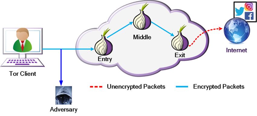
2
model, so we explore how to create adversarial examples for • We show how algorithms for generating adversarial ex-
network traffic. We find that adversarial examples have three amples in computer vision fail as a defense in the WF
attributes that are valuable for defending against WF: i) high setting, motivating more robust techniques.
misclassification rates, ii) small perturbations, which ensure • Our evaluation shows that Mockingbird significantly re-
a low overhead, and iii) transferability. The transferability duces accuracy of the state-of-the-art WF attacks hardened
property [4], in which some adversarial examples can be with adversarial training from 98% to 38%-58% attack
made to reliably work on multiple models [16], [17], makes accuracy, depending on the scenario. The bandwidth over-
it possible to defend against unknown attacks and potentially head is 58% for full-duplex traffic, which is better than
even ones with more advanced capabilities. both W-T and WTF-PAD.
In this paper, we introduce Mockingbird,1 a defense strategy • We show that Mockingbird makes it difficult for an at-
using adversarial examples for network traffic traces, which we tacker to narrow the user’s possible sites to a small set. The
call adversarial traces. In the WF context, we cannot simply best attack can get at most 72% Top-2 accuracy against
perform a straightforward mapping of adversarial examples to Mockingbird, while its Top-2 accuracy on W-T and WTF-
network traffic. As it is the reverse of when the adversary PAD is 97% and 95%, respectively.
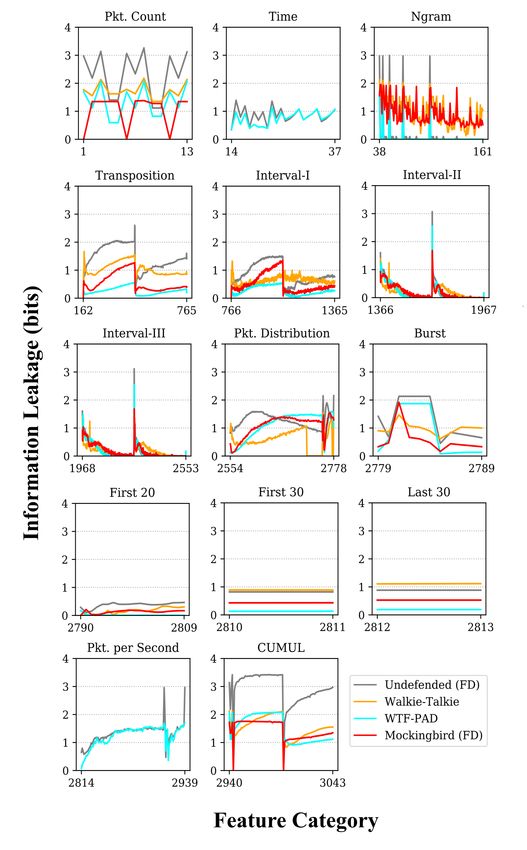
is applying the adversarial examples, the WF attacker gets • Using the WeFDE framework [20], we measure the infor-
to know what the WF defender is doing to generate the mation leakage of Mockingbird, and find that it has less
examples. In particular, he can use the defense as implemented leakage for many types of features than either W-T or
in open-source Tor code to generate his own adversarial traces WTF-PAD.
and then use them to train a more robust classifier. This
Our investigation of this approach provides a promising first
adversarial training approach has been shown to be effective
step towards leveraging adversarial examples to undermine
when the classifier knows how the adversarial traces are being
WF attacks and protect user privacy online.
generated [18].
To address this, we propose a novel technique to generate II. T HREAT & D EFENSE M ODEL
adversarial traces that seeks to limit the effectiveness of
A. Threat Model
adversarial training. In particular, we increase the randomness
of the search process and reduce the influence of the design We assume that the client browses the Internet through
and training of the targeted deep learning model in finding the Tor network to hide her activities (see Figure 1). The
a good adversarial example. To this end, as we search for adversary of interest is local, which means the attacker is
the new trace, we select a random target trace and gradually positioned somewhere in the network between the client and
reduce the distance from the modified trace to the target. We Tor guard node. The attacker is assumed to already know the
also change to other randomly selected targets multiple times identity of the client. His goal is to detect the websites that the
during the search. The deep learning model is only used to client is visiting. A local adversary can be an eavesdropper on
give a confidence value on whether the current trace fools the the user’s local network, local system administrators, Internet
classifier, and we do not access the loss function, the logits, or service provider, any networks between the user and the entry
any other aspect of the model. The resulting adversarial traces node, or the operator of the entry node. The attacker is passive,
can go in many different directions from the original source meaning that the he only observes and records the traffic traces
traces instead of consistently following the same paths that that pass through the network. He does not have the ability to
result from, e.g., following the gradient of the loss function. drop, delay, or modify real packets in the traffic stream.
In this way, the technique selects paths that are hard to find In a website fingerprinting (WF) attack, the attacker feeds
through adversarial training. Further, each new trace generated the collected network traffic into a trained machine-learning
from the same source typically ends near a different target each or deep-learning classifier. For the purpose of training, the
time, helping to reduce the attacker’s Top-k accuracy. WF attacker first needs to collect traffic of various sites by
operating a Tor client. Since is not feasible to collect traffic
Extensive evaluation shows that Mockingbird2 reliably
for all the sites on the web, the attacker identifies a set of
causes misclassification in a deep learning classifier hardened
monitored sites that he wants to track. The attacker limits the
with adversarial training using moderate amounts of band-
scope of his attack to the identification of any website visits
width overhead. Our results hold even when the attacker uses a
that are within the monitored set. The set of all other sites is
significantly more powerful classifier than the target classifier
known as the unmonitored set.
used by Mockingbird to produce the adversarial examples.
WF attacks and defenses are evaluated in two different
Contributions. In summary, the key contributions of this work settings: closed-world and open-world. In the closed-world
are as follows: setting, we assume that the client is limited to visiting only
• We propose Mockingbird, the first WF defense to leverage the monitored sites. The training and testing set used by the
the concept of adversarial examples. attacker only include samples from the monitored set. The
closed-world scenario models an ideal setting for the attacker
and is not indicative of the attack’s real-world performance.
1 The Northern mockingbird imitates the calls of a wide range of other birds,
From the perspective of developing a WF defense, demonstrat-
and one of its call types is known as a chatburst that it uses for territorial
defense: https://en.wikipedia.org/wiki/Northern mockingbird ing the ability to prevent closed-world attacks is thus sufficient
2 This work is an extended version of a short paper [19]. to show its effectiveness.3
In contrast, the open-world scenario models a more realistic in the closed-world setting using a dataset of 100 sites with
setting in which the client may visit websites from both 1,000 instances each. They also examined the effectiveness
the monitored and unmonitored sites. In this setting, the of their model against WF defenses, where they showed
attacker trains on the monitored sites and a representative (but that their model can achieve concerningly high performance
not comprehensive) sample of unmonitored sites. The open- against even some defended traffic. Most notably, their attack
world classifier is then evaluated against both monitored and achieved 90% accuracy against WTF-PAD [14] and 98% Top-
unmonitored sites, where the set of unmonitored sites used for 2 accuracy against Walkie-Talkie [15].
testing does not intersect with the training set. Var-CNN. Recently, Bhat et al. [8] developed a more sophis-
ticated WF attack based on the ResNet CNN architecture and
B. Defense Model attained 98.8% closed-world accuracy.
The purpose of a WF defense is to prevent an attacker We evaluated Mockingbird on both the DF model and Var-
who observes a traffic trace from determining accurately to CNN model in the black-box setting.
which site the trace belongs. To achieve this, the real traffic
stream must be manipulated in some way. Because traffic B. WF Defenses
is bidirectional, the deployment of a successful WF defense
requires participation from both the client and a cooperating To defeat WF attackers, researchers have explored various
node in the Tor circuit. We call this node the bridge.3 To defense designs that generate cover traffic to hide the features
defend against eavesdroppers performing WF attacks, the present in website traffic. WF defenses are able to manipulate
bridge could be any node located between the adversary and the traffic stream with two operations: sending dummy packets
the client’s destination server, making it so that the adversary and delaying real packets. These manipulations, however,
only has access to the obfuscated traffic stream. Since the come at a cost: sending dummy packets adds an additional
guard node knows the IP address of the client and can thus bandwidth overhead to the network, while delaying packets
act as as a WF adversary, it is better to set up the bridge at adds latency overhead that directly impacts the time required
the middle node, which cannot directly identify the client. to load the page. Several studies have thus tried to balance
the trade-off between the WF defense’s overhead and efficacy
of the defense against WF attacks. In this section, we review
III. BACKGROUND & R ELATED W ORK
these WF defenses.
A. WF Attacks
Constant-rate padding defenses. This family of defenses
Website fingerprinting attacks have applied a variety of transmits traffic at a constant rate in order to normalize trace
classifiers. The three best attacks based on manual feature characteristics. BuFLO [25] is the first defense of this kind,
engineering are k-NN [21], CUMUL [22], and k-FP [23], and it sends the packets in the same constant rate in both
which all reached over 90% accuracy in closed-world tests on directions. The defense ends transmission after the page has
datasets with 100 samples per site. In the rest of this section, finished loading and a minimum amount of time has passed.
we examine the more recent deep-learning-based WF attacks. The overhead of the traffic is governed by both the transmis-
SDAE. The first to investigate using deep-learning techniques sion rate and the minimum time threshold for the stopping
for WF were Abe and Goto [24], who developed an attack condition. Moreover, although the defense covers fine-grained
based on Stacked Denoising Autoencoders (SDAE). Their features like burst information, course-grained features like the
model was trained on raw packet direction, represented by volume and load time of the page still leak information about
a sequence of “+1” and“-1” values for outgoing and incoming the website. Tamaraw [13] and CS-BuFLO [12] extend the
packets, respectively. Despite this innovation, their attack BuFLO design with the goal of addressing these issues. To
achieved a lower accuracy rate than the previous state-of-the- provide better cover traffic, after the page is loaded, Tamaraw
art attacks at only 88% in the closed-world setting. keeps padding until the total number of transmitted bytes is
a multiple of a fixed parameter. Similarly, CS-BuFLO pads
Automated Website Fingerprinting (AWF). Rimmer et al. [10]
the traffic to a power of two, or to a multiple of the power
proposed using deep learning to bypass the feature engineering
of the amount of transmitted bytes. All of these defenses are
phase of traditional WF attacks. To more effectively utilize
expensive, requiring two to three times as much time as Tor to
DL techniques, they collected a very large dataset of 900 sites
fetch a typical site and more than 100% bandwidth overhead.
with 2,500 trace instances per site. They applied several differ-
ent DL architectures—SDAE, Convolutional Neural Network Supersequence defenses. This family of defenses depends on
(CNN), and Long Short-Term Memory (LSTM)—on the traffic finding a supersequence for traffic traces. To do this, these
traces. They found that their CNN model outperforms the other defenses first cluster websites into anonymity sets and then
DL models they developed, obtaining 96% accuracy in the find a representative sequence for each cluster, such that
closed-world setting. it contains all the traffic sequences. All the websites that
belong to the same cluster are then molded to the representa-
Deep Fingerprinting (DF). Sirinam et al. [9] developed a
tive supersequence. This family includes Supersequence [21],
deeper CNN model that reached up to 98% accuracy rate
Glove [11], and Walkie-Talkie [15]. Supersequence and Glove
3 Tor bridges are usually used for evading censorship, but they can be used use approximation algorithms to estimate the supersequence of
for prototyping WF defenses such as used in WTF-PAD [14]. a set of sites. The traces are then padded in such a way so as4
to be equivalent to its supersequence. However, applying the The idea of creating adversarial examples is to modify
molding directly to the cell sequences creates high bandwidth samples from one class to make them be misclassified to
and latency costs. Walkie-Talkie (WT) differs from the other another class, where the extent of the modification is limited.
two defenses in that it uses anonymity sets of just two sites, More precisely, given an input sample x and target class t
and traces are represented as burst sequences rather than cell that is different from actual class of x (t 6= C ∗ (x)), the goal
0
sequences. Even with anonymity sets of sizes of just two, is to find x which is close to x according to some distance
0 0
this produces a theoretical maximum accuracy of 50%. Wang metric and C(x ) = t. In this case, x is a targeted adversarial
and Goldberg report just 31% bandwidth overhead for their example since it is misclassified to a particular target label t.
defense, but also 34% latency overhead due to the use of half- An untargeted adversarial example, on the other hand, may be
duplex communication. Against WT, the DF attack achieved misclassified to any other class except the true class (C ∗ (x)).
49.7% accuracy and 98.4% top-2 accuracy, meaning that it In response to the threat of adversarial examples, many
could effectively identify the two sites that were molded defense techniques have been introduced to make classifiers
together but not distinguish between them [9]. more robust against being fooled. Recent research [28], [29]
WTF-PAD. Shmatikov and Wang [26] proposed Adaptive shows that almost none of these recent defense techniques are
Padding (AP) as a countermeasure against end-to-end traffic effective. In particular, we can generate adversarial examples
analysis. Juarez et al. [14] proposed the WTF-PAD defense as that counter these defense techniques by including the defense
an adaptation of AP to protect Tor traffic against WF attacks. techniques directly into the optimization algorithm used to
WTF-PAD tries to fill in large delays between packets (inter- create the adversarial examples. We can also overcome many
packet arrival times). Whenever there is a large inter-packet defense approaches by simply increasing the amount of per-
arrival time (where ”large” is determined probabilistically), turbation used [30].
WTF-PAD sends a fake burst of dummy packets. This ap-
B. Properties of Adversarial Examples
proach does not add any artificial delays to the traffic. Juarez
et al. show that WTF-PAD can drop the accuracy of the k- Adversarial examples have three major properties that make
NN attack from 92% to 17% with a cost of 60% bandwidth them intriguing for us in WF defense: i) robust misclassifica-
overhead. Sirinam et al. [9], however, show that their DF attack tion, ii) small perturbations, and iii) transferability. We now
can achieve up to 90% accuracy against WTF-PAD in the explain the effect of each of these properties in a WF defense.
closed-world setting. Robust Misclassification. An effective defense should be
Application-level defenses. Cherubin et al. [27] propose the able to fool a trained WF classifier consistently in real-world
first WF defenses designed to work at the application layer. conditions. Adversarial examples have been shown to work
They proposed two defenses in their work. The first of these reliably and robustly for images, including for cases in which
defenses, ALPaCA, operates on the webserver of destination the viewpoint of the camera cannot be fully predicted, such
websites. ALPaCA works by altering the size distribution for as fooling face recognition [31] and self-driving cars [32].
each content type, e.g. PNG, HTML, CSS, to match the profile Small Perturbations. To fool the classifier, the defense will
for an average onion site. In the best case, this defense has 41% add padding packets to the original network traffic. Ideally, a
latency overhead and 44% bandwidth overhead and reduces WF defense should be lightweight, meaning that the number
the accuracy of the CUMUL attack from 56% to 33%. Their of padding packets should be constrained to keep bandwidth
second defense, LLaMA, operates exclusively on the client. It consumption low. By using small perturbations to achieve
adds random delays to HTTP requests in an effort to affect misclassification, an effective WF defense based on adversarial
the order of the packets by manipulating HTTP request and examples can also be lightweight.
responses patterns. LLaMA drops the accuracy of the CUMUL Transferability. Recent research shows that defenses such as
attack on Onion Sites from 56% to 34% at cost of 9% latency WTF-PAD [14] and W-T [15], which defeated the state-of-the-
overhead and 7% bandwidth overhead. art attacks available at that time, are seriously underminded
by the more recent and advanced attacks [6], [9]. Given that
IV. P RELIMINARIES the attacker could use any classifier for WF, the defense
should extend beyond current attacks to other possible attacks
A. Adversarial Examples as well. Adversarial examples provide the ability for this
Szegedy et al. [4] were the first to discover that otherwise due the the transferability property, which indicates that they
accurate ML and DL image classification models could be can be designed to attack a given classifier and at least
fooled by image inputs with slight perturbations that are sometimes also fool other classifiers [16]. Further, there are
largely imperceptible to humans. These perturbed inputs are techniques that work in a black-box setting, where the classifier
called adversarial examples, and they call into question the is completely unknown to the attacker [17], [33]. This property
robustness of many of the advances being made in machine is very important for WF defense, since we cannot predict the
learning. The state-of-the-art DL models can be fooled into attacker’s classifier in advance.
misclassifying adversarial examples with surprisingly high
confidence. For example, Papernot et al. [17] show that C. Adversarial Training
adversarial images cause a targeted deep neural network to Recent research shows that adversarial training increases the
misclassify 84% of the time. robustness of a model by incorporating adversarial examples in5
scenario represents the scenario most typically seen in the
adversarial example literature, in which the classifier has not
been trained on any adversarial instances. In this scenario,
we generated the adversarial examples against a target model
and tested them against the different WF attacks trained on
the original traffic traces. We find that our adversarial traces
Fig. 2: A visual representation of bursts. are highly effective against the WF attacks. The accuracy of
DF [9] is reduced from 98% to 3%, and the accuracy of
CUMUL [22] drops from 92% to 31%. The adversarial traces
the training data [34], [18]. The idea is to train a network with generated using this method are highly transferable, as we
adversarial examples so that they can be classified correctly. generated them against a target CNN model similar to the one
This approach is limited, as it does not adapt well to techniques proposed by Rimmer et al. [10], and they are effective against
for generating adversarial examples that haven’t been trained both DF and CUMUL.
on. In the WF setting, however, the classifier has the advantage Unfortunately, this scenario is not realistic, as it is likely
of knowing how the adversarial examples are being generated, (and usually assumed) that the attacker can discern what type
as they would be part of the open-source Tor code. Thus, of defense is in effect and train on representative samples. This
adversarial training is a significant concern for our system. is represented by the with-adversarial-training scenario. In this
scenario, the C&W technique fails completely, with the DF
D. Data Representation attack reaching 97% accuracy. In addition, we also investigated
Following the previous work [14], [15], [9], we model the a method that combines aspects of our Mockingbird system
traffic trace as a sequence of incoming (server to client) and with C&W, but this also proved to be ineffective as a WF
outgoing (client to server) bursts. The incoming and outgoing defense. We discuss the details of these evaluations in the
packets are represented as −1 and +1, respectively. We define Appendices.
a burst as a sequence of consecutive packets in the same The results of this evaluation led to a very important insight:
direction. An example of the burst representation is shown the scenario in which the effectiveness of adversarial examples
in Figure 2. Given this, we can increase the length of any burst are typically evaluated is notably different than that of a WF
by sending padding packets in the direction of the burst. We defense. In particular, the attacker has the advantage of going
cannot, however, decrease the size of the bursts by dropping second, which means that the classifier can be designed and
real packets due to the retransmissions this would cause, trained after the technique is deployed in Tor. Thus, techniques
changing the traffic patterns and adding delays for the user. that excel at producing adversarial examples for traditional
attacks are poorly suited for our problem. In response to this
V. Mockingbird D ESIGN discovery, we focused our efforts on the development of a new
We now motivate and describe the design of the Mocking- technique designed specifically for our needs. We discuss our
bird defense in detail. We start by evaluating the performance method in the following section.
given by adapting existing adversarial-example techniques,
which are not effective against adversarial training, and then B. Generating Adversarial Traces
examine the Mockingbird design in detail.
A. Applying Existing Methods in WF Defense
Several different algorithms have been proposed for gener-
ating adversarial examples within the field of computer vision,
including the Fast Gradient Sign Method (FGSM) [35], the It-
erative Fast Gradient Sign Method (IGSM) [36], the Jacobian-
Based Saliency Map Attack (JSMA) [37], and optimization-
based methods [29], [33]. For our initial exploration of ad- Fig. 3: Mockingbird Architecture.
versarial examples in WF defense, we examine the technique
proposed by Carlini and Wagner (C&W) [16]. We now introduce Mockingbird, a novel algorithm to gen-
This method is shown to defeat the defensive distillation erate adversarial traces that more reliably fool the classifier in
approach of blocking adversarial examples [38]. The algo- the adversarial training setting. The ultimate goal is to generate
rithm is successful with 100% probability. We modified their untargeted adversarial traces that cause the classifier to label a
technique to suit our needs to generate adversarial traces out traffic trace as coming from some site other than the original
of the burst sequences. This algorithm is designed to work on site, i.e. to generate an untargeted sample. We find, however,
images, which are 2D, so we modified it to work on 1D traffic that it is more effective to generate targeted samples, i.e. to
traces. select specific other sites for the current sample to attempt to
We evaluated the performance of this technique in two dif- mimic. Much like its namesake (the bird), Mockingbird uses
ferent WF attack scenarios: without-adversarial-training and a variety of targets, without much importance on which target
with-adversarial-training. The without-adversarial-training it mimics at any given moment.6
To defend a given trace, the source sample, Mocking- Algorithm 1: Generate Adversarial Traces.
bird first generates a set of potential target traces selected Input : S – set of sensitive sites
randomly from the traces of various sites other than the source D – detector f (x)
α – amplifier
site. It then randomly picks one of these traces as the target δ – iterations before selecting a new target
sample and gradually changes the source sample to get closer τc – confidence threshold
to the target sample. The process stops when a trained classifier τD – perturbation threshold
N – maximum number of iterations
called the detector determines that the class of the sample p – number of targets to pick for the pool
has changed (see Figure 3). Note that it does not need to Is – instance of site s to protect
have changed to the target sample’s class, as the goal is to bj – bursts in Is , j ∈ [1, . . . , n]
Output: Is0 – altered (adversarial) trace of Is
generate an untargeted adversarial trace. The amount of change
1 Ys ← D(Is ) // label of Is
applied to the source sample governs the bandwidth overhead 2 Ps ← random(p, S − {s}) // target pool
of Mockingbird, and as such should be minimized. 3 IT ← argminD(Is , I) // target sample
Unlike most other algorithms used to generate adversarial I∈Ps
examples, Mockingbird does not focus on the loss function 4 Is0 ← Is
5 for iter in [1, . . . , N ] do h
(like FGSM and IGSM) or logits (like Carlini & Wagner) 0
∂D(IS ,IT )
i
6 ∇(−D(Is0 , IT )) ← − ∂b
of the detector network. Instead, it aims to move the source j j∈[1,··· ,n]
sample towards the target sample and only uses the detector ∂D(Is0 ,IT )
7 ∆←α× ∇(−D(Is0 , IT )), where − ∂bj
>0
network to estimate the confidence with which the trace is 8 Is0 ← Is0 + ∆
misclassified. This lessens the reliance on the shape of the de- /* Compute the label and confidence for Is0 */
tector network and helps to generate adversarial traces that are 9 Ys0 , P (Is0 ) ← D(Is0 )
more robust against adversarial training. As we demonstrate /* End if the source class confidence is low */
in the Supplementary Materials, using an optimization method 10 if Ys0 6= Ys and P (Is0 ) < τc then
11 break
to move towards the target sample results in a system that is
/* Pick a new target after δ iterations */
much less robust. 12 if i mod δ = 0 and Ys0 = Ys and Is0 − Is < τD then
Mockingbird Algorithm: We assume that we have a set of 13 Ps ← random(p, S − {s}) // new target pool
14 IT ← argminD(Is , I) // new target sample
sensitive sites S that we want to protect. We train a detector I∈Ps
f (x) on a set of data from S. We discuss the design and 15 return Is0
training of f (x) in Section VI. We consider traffic trace Is
as an instance of source class s ∈ S. Our goal is to alter Is
to become Is0 such that it is classified to any other class t, To make the source sample leave the source class, we
t = f (I 0 s ) and t 6= s. change it with the minimum amount of perturbation in the
direction that makes it closer to the target (It ). We define ∆
Is is a sequence of the bursts, Is = bI1 , bI2 , ..., bIn , where n
is the number of the bursts. Burst is defined as the sequence of as the perturbation vector that we add to the source sample to
packets in a direction (i.e. incoming or outgoing) [8], [9], [21]. generate its defended form Isnew .
The length of each burst (i.e. number of packets in each burst),
∆ = [δ0 , δ1 , · · · , δn ] (δi >= 0) (3)
bIi , makes the sequence of bursts. Usually, the number of
packets in each burst vary widely. The only allowed operation
on a burst bIi is to add some positive values δi >= 0 to that Isnew = Is + ∆ (4)
burst, bIi = bIi +δi . The reason for using δi >= 0 is that we can
only increase the size of a burst. If δi < 0, that would mean We need to find a ∆ that adds the least amount of per-
we should drop some packets to reduce the size of a burst, turbation to the source sample while still making it closer
and dropping real packets means losing data and requires re- to the target sample. Therefore, we find ∆ that minimizes
transmission of the dropped packet. To protect source sample distance D(Isnew , IT ). To do so, we compute the gradient of
Is , we first select τ potential target samples from other classes the distance with respect to the input. Note that most work in
ti 6= s. We then select the target t as the one nearest to the adversarial example generation uses the gradient of the loss
source sample based on the l2 norm distance4 . This helps to function of the discriminator network rather than distance,
minimize overhead, as we will move the source towards the and this may make those techniques more sensitive to the
design and training of the classifier. The gradient points in
target. More formally, we pick a target pool Ps of p random the direction of steepest ascent, which would maximize the
samples from other classes, Ps = I 0 0 , I 1 1 , .., I p m , where
I j i is the j-th sample in the target pool and belongs to target distance. Therefore, we compute the gradient of the negative
class ti 6= s. The target sample It is selected as shown in of the distance with respect to the input, and we modify the
Equation 1. source sample in that direction towards the target sample. In
particular:
It = argminD(Is , I) (1)
I∈Ps ∂D(I, IT ) ∂D(I, IT )
∇(−D(I, IT )) = − = − (5)
D(x, y) = l2 (x − y) (2) ∂I ∂bi i∈[0,··· ,n]
4 We also performed some preliminary experiments with Manhattan dis-
tance and found no significant improvement. Where bi is the i-th burst in input I.7
To modify the source sample, we change bursts such that
Cumulative Fraction
their corresponding values in ∇(−D(I, IT )) are positive. Our 1
perturbation vector ∆ is: 0.8
0.6
( Half-Duplex
−α × ∂D(I,I
∂bi
T)
− ∂D(I,I
∂bi
T)
>0 0.4
δi = (6) Full-Duplex
∂D(I,IT ) 0.2
0 − ∂bi 60
0
where α is the parameter that amplifies the output of the 0 250 500 750 1,000 1,250 1,500
gradient. The choice of α has an impact on the convergence Number of Bursts
and the bandwidth overhead. If we pick a large value for α, we
Fig. 4: CDF of the number of bursts in the full-duplex and
will take bigger steps toward the target sample and add more
half-duplex traces.
overhead, while small values of α require more iterations to
converge. We modify the source sample by summing it with TABLE I: Dataset Split: Adv Set (A) & Detector Set (D).
∆, (Isnew = Is + ∆). We iterate this process, computing ∆ FD: Full-Duplex, HD: Half-Duplex, C: Class, I: Instance,
for Is and updating the source sample at each iteration until CW:Closed-World, OW: Open-World.
we leave the source class, f (Isnew ) 6= s or the number of
Adv Set A Detector Set D CW OW
iterations passes the maximum allowed iterations. Note that at
(C × I) (C × I) Total
the end of each iteration, we update the current source sample FD 95×259 95×259 95×518 40,716
with the modified one, Is = Isnew . Leaving the source class HD 83×360 83×360 83×720 40,000
means that we have less confidence on the source class. So we
fix a threshold value, τc , for measuring the confidence. If the
confidence of the detector on the source class is less than the
threshold (fs (Isnew ) < τc ), Mockingbird will stop changing and the instances that start with an incoming packet, since the
the source sample (Is ). client should send the first packet to start the connection.
As we only increase the size of the bursts where Full-Duplex (FD): The CW dataset contains 95 classes with
− ∂D(I,I
∂bi
T)
> 0, we may run into cases that after some 1000 instances each. After preprocessing, we end up with
iterations ∇(−D(I, IT )) does not have any positive values or 518 instances for each site. The OW dataset contains 40,716
all the positive values are extremely small such that they do not different sites with 1 instance each.
make any significant changes to Is . In such cases, if Isnew −Is Half-Duplex (HD): The CW dataset contains 100 sites with
is smaller than a threshold τD for λ consecutive iterations 900 instances each. After preprocessing, we ended up with 83
(we used λ = 10), and we are still in the source class, we classes with 720 instances per class. The OW data contains
select a new target. In particular, we effectively restart the 40,000 sites with 1 instance each.
algorithm by picking a new pool of potential target samples,
selecting the nearest target from the pool, and continuing the An additional consideration is that we must use a fixed
process. It is to note that, the source sample at this point is size input to our model [9]. To find the appropriate size, we
already in the changed form Isnew and the algorithm starts consider the distribution of burst sequence lengths within our
changing from Isnew . In this process, the confusion added by datasets. Figure 4 shows the CDF of the burst sequence lengths
Mockingbird in the final trace is proportional to the number of for both the HD and FD datasets. More than 80% of traces
targets changed to reach the final adversarial trace. The pseudo have fewer than 750 bursts for the HD CW dataset, and more
code of Mockingbird algorithm is presented in Algorithm 1. than 80% of the traces for the CW FD dataset have fewer
than 500 bursts. We found that using 1500 bursts on both HD
and FD datasets provides just 1% improvement on accuracy
VI. E VALUATION for the DF attack compared to using 750 bursts.To decrease
A. Datasets the computational cost for generating adversarial examples,
we use an input size of 750 bursts for both the FD and HD
We apply Mockingbird to generate adversarial examples on datasets. Note that the attacker in our evaluations uses 10,000
the traffic traces at the burst level. We can get the burst packets rather than bursts.
sequence of the traffic traces from both full-duplex (FD) In our evaluation, we need to address the needs of both
and half-duplex (HD) communication modes. Walkie-Talkie Mockingbird and the adversary to have training data. We thus
(W-T) [15] works on HD communication, and it finds the break each dataset (full-duplex (FD) and half-duplex (HD))
supersequences on the burst level. In our experiments, we use into two non-overlapping sets: Adv Set A and Detector Set D
burst sequences for both FD and HD datasets. (see Table I). A and D each contain half of the instances of
Data Source: We use both the closed-world (CW) and open- each class. This means, in both A and D, 259 instances for
world (OW) FD and HD traffic traces provided by Sirinam et each of 95 classes for FD data and 360 instances for each of
al. [9]. The websites classes from the monitored set are from 83 classes for HD data.
the top sites in Alexa [39].
Preprocessing Data: In our preprocessing phase, we filter the B. Experimental Method
data by removing any instances with fewer than 50 packets Mockingbird needs to train a detector f (x) with instances8
TABLE II: Hyperparameter Tuning on DF and Var-CNN attack and the remaining 10% for testing for each of the settings. To
models for Black-box attacks. represent the data in the attack models, we follow the prior
Final work [8], [9], [21], [22], [23] and represent the data as an
Hyperparameters Choices DF Var-CNN 1-D vector of +1 and −1 for outgoing and incoming packets,
Training Epoch [30, 50, 100, 150] 100 100 respectively. We use a fixed length of 5000 for each instance of
Batch Size [32, 64, 128, 256] 32 32
the class following the prior work. Instances that do not have
Optimizer [Adam, Adamax] Adamax Adamax
Learning Rate [0.001, 0.002, 0.003] 0.002 0.002 5,000 packets are padded with zero, and the instances that
Activation Fn. [ReLU, ELU] ReLU, ELU ReLU have length more than 5,000 are truncated to that particular
length.
As black-box setting is the most realistic attack setting
of a variety of sites to generate adversarial traces. We use to evaluate a defense, we perform hyperparameter tuning on
both Rimmer et al.’s CNN model [10], which we refer to the two deep-learning based attack models: DF [9] and Var-
as AWF, and Sirinam et al.’s more powerful DF model [9] CNN [8]. However, we exclude the hyperparameters choices
for detector models. We train these models on the traces of that have been explored in prior work and did not provide
the Detector Set. Sirinam et al. suggest using an input size any improvement in the attack accuracy. Such hyperparameters
of 5,000 packets, but our padded traces have more traffic, include the SGD and RMSPros optimization functions, and the
so we use an input size of 10,000 packets, which is the tanh activation function.
80th percentile of packet sequence lengths in our defended We start our search with the default model and continue
traces. Sample from the Detector Set are only used to train the tuning each hyperparameter one by one. First, we perform
detector. The source samples from Adv Set (Is ∈ A) are used several sets of experiments with different training epochs
to generate adversarial traces for the training, validation, and for both full-duplex (FD) and half-duplex (HD) with both
testing of the adversary’s classifier. To evaluate the defended DF [9] and Var-CNN [8] models. Then, the best training epoch
traffic, we reform the defended traces from the burst level number is used for the experiments to search for the next set of
representation to the direction level representation where “+1” hyperparameters. Table II shows the hyperparameters and the
and “-1” indicate outgoing and incoming packets, respectively, choices of our hyperparameter tuning process. In our tuning
following the previous research. process, we found that the tuned DF and Var-CNN models
work better for the FD traces defended by Mockingbird and
Attack Settings. We test with two different settings, white- default DF and Var-CNN models work better for the HD traces
box and black-box. In all of the evaluations, the classifier is defended by Mockingbird.
trained using adversarial training, where the attacker has full
access to the defense and uses it to generate defended samples Top-k Accuracy. Most prior works have focused their analysis
for each class in the monitored set. on Top-1 accuracy, which is normally referred to simply as
the accuracy of the attack. We argue that Top-1 accuracy
• White-box: In the white-box setting, we assume that that does not provide a full picture of the effectiveness of a
defense uses the same network architecture for the detector defense, as an attacker may use additional insights about their
as the attacker uses to perform WF attacks. We use this target (language, locale, interests, etc.) to further deduce what
overly optimistic scenario only for parameter search to website their target is likely to visit.
identify values for α and number of iterations, where we As such, it is desirable to examine the accuracy of Top-k
use DF as both the detector and the attack classifier. predictions, where k is the number of top-ranked classes in the
• Black-box: In the black-box setting, the defender and prediction. In evaluations of WF, we are particularly interested
the attacker use two different neural networks, i.e. the in the Top-2 accuracy. A high Top-2 accuracy indicates that
defender uses one model for the detector, while the the classifier is able to reliably determine the identity of a
attacker uses another model for performing WF attacks. trace to just two candidate websites. This is a threat to a user
We evaluate Mockingbird in the black-box setting by using even when the attacker is unable to use additional information
the AWF CNN model [10] as the detector and both the DF to predict the true site. The knowledge that the target may
model [9] and Var-CNN [8] as attacker models. Since DF be visiting a sensitive site is actionable and can encourage the
and Var-CNN are more powerful than the simple AWF attacker to expend additional resources to further analyze their
model [9], [8], this tests the case that the attacker has target.
greater capabilities than are known to the defender. These
evaluations show the extent to which adversarial examples Target Pool. Mockingbird changes the source sample toward
generated by Mockingbird transfer to other classifiers. a target sample drawn randomly from our target pool. The
detector determines whether the perturbed source sample is
• Traditional ML Attack: We also evaluate Mocking-
still in the source class. We are interested to know how the
bird against tradition machine-learning (ML) attacks such
algorithm performs if we fill the target pool with instances of
as CUMUL [22], k-FP [23], and k-NN [21], all of which
sites that the detector has been trained on and has not been
reach over 90% accuracy on undefended Tor using closed-
trained on. We examine the bandwidth overhead and reduction
world datasets with 100 samples per class.
in the attack accuracy of traces protected by Mockingbird in
Training and Hyperparameter Tuning. To perform the at- these two scenarios.
tacks, we use 80% of the data for training, 10% for validation, • Case I: We fill the target pool with instances from the9
(a) Confidence Threshold Value (τc ) (b) Perturbation Threshold Value (τD )
Fig. 5: Full-duplex: the attacker’s accuracy and the bandwidth overhead (BWO) of the generated samples as we vary the
probability threshold value (Figure 5a) and perturbation threshold value (Figure 5b).
Accuracy
Accuracy
Accuracy
0.75 Case I 0.75 0.75 α=5 0.75 0.75 α=5 0.75
BWO
BWO
BWO
Case II α=7
0.65 0.65 0.65 α=7
0.65 0.65 0.65
0.55 0.55 0.55 0.55 0.55 0.55
0.45 0.45 0.45 0.45 0.45 0.45
0.35 0.35 0.35 0.35 0.35 0.35
0.25 0.25 0.25 0.25 0.25 0.25
1 3 5 7 100 200 300 400 500 100 200 300 400 500
α Value Number of Iterations Number of Iterations
(a) α Value for full-duplex (b) Case I (c) Case II
Fig. 6: Full-duplex: the attacker’s accuracy and the bandwidth overhead (BWO) of the generated samples as we vary the α
value (Figure 6a) and number of iterations (Figure 6b and 6c).
Adv Set. Therefore, both source samples (Is ∈ A) and C. Tuning on Full-Duplex Data
target samples (I j i ∈ A which Ti 6= s) are from the The full-duplex version of Mockingbird is the easier to
Adv Set. In this case, we assume that the detector has deploy and leads to lower latency costs than the half-duplex
been trained on the target classes, which makes it more version [15], so we lead with the full-duplex results. We use
effective at identifying when the sample has left one class the white-box setting for simplicity.
for another. This may be less effective, however, if the
adversary trains on the source class but none of the other Choice of Threshold Values. There are two thresholds values
target classes used in detection. in Mockingbird algorithm: i) a confidence threshold value (τc )
that limits the confidence on the generated trace belonging to
• Case II: We fill the target pool with instances from
the correct class, and ii) a perturbation threshold value (τD )
unmonitored sites that are not in the Adv Set. We select
that limits the amount of change in a generated trace. Intu-
the target samples (I j i ) from the open-world dataset. The
itively, the smaller the value of τc , the less likely it is that the
source samples (Is ) are from Adv Set, and we generate
attacker could succeed, at the cost of higher average bandwidth
their defended forms. In this case, we assume the detector
overhead. By contrast, changing τD directly manipulates the
has not been trained on the target samples, so it may be
maximum bandwidth overhead, where lower τD would reduce
less effective in identifying when the sample leaves the
bandwidth cost but also typically result in an improved chance
class. That may make it more robust when the attacker
of attack success.
also trains on a different set of classes in his monitored
While we experiment with different τc values, we fix the
set.
τD = 0.0001, α = 5, and number of iterations to 500. We
can see from Figure 5a that lower values of τc lead to lower
Case I may be realistic when the defender and the attacker
accuracy and higher bandwidth. τc = 0.01 provides a good
are both concerned with the same set of sites, such as protect-
tradeoff point, so we select it for our following experiments.
ing against a government-level censor with known patterns
Following the same procedure, we perform experiments
of blocking, e.g. based on sites it blocks for connections not
with different τD values. As expected, and as shown in
protected by Tor. Case II is a more conservative estimate of
Figure 5b, lower τD values lead to lower bandwidth but higher
the security of Mockingbird and thus more appropriate for our
attack accuracy. We choose τD = 0.0001 as a good tradeoff
overall assessment.
for our following experiments.
We generate defended samples with various settings. We Choice of α. Figure 6a shows the bandwidth overhead and
vary α to evaluate its effect on the strength of the defended attack accuracy of full-duplex data with respect to α values for
traces and the overhead. We also vary the number of iterations both Case I (solid lines) and Case II (dashed lines) with 500
required to generate the adversarial traces. Each iteration iterations. As expected, the bandwidth overhead increases and
moves the sample closer to the target, improving the likelihood the attack accuracy decreases as we increase α, with longer
it is misclassified, but also adds bandwidth overhead. steps towards the selected targets. For Case I, the adversary’s10
(a) Confidence Threshold Value (τc ) (b) Perturbation Threshold Value (τD )
Fig. 7: Half-duplex: the attacker’s accuracy and the bandwidth overhead (BWO) of the generated samples as we vary the
probability threshold value (Figure 7a) and perturbation threshold value (Figure 7b).
Accuracy
Accuracy
0.75 0.75 0.75 0.75
BWO
BWO
Case I
0.65 0.65 Case I
0.65 0.65
Case II 0.55 0.55 Case II 0.55 0.55
0.45 0.45 0.45 0.45
0.35 0.35 0.35 0.35
0.25 0.25 0.25 0.25
3 1 5 7 100 200 300 400 500
α Value Number of Iterations
Fig. 8: Half-duplex: attacker accuracy and bandwidth overhead Fig. 9: Half-duplex: attacker accuracy and bandwidth overhead
(BWO) as α varies. (BWO) as the number of iterations varies.
accuracy against Mockingbird with α=5 and α=7 are both
35%, but the bandwidth overhead is lower for α = 5 at 56% more precise control over burst patterns such that we can
compared to 59% for α = 7. For Case II, the adversary’s achieve reduced attacker accuracy as shown in the following
accuracy and the bandwidth overhead are both slightly lower white-box results.
for α=5 than that of α=7. From these findings, we fix α=5 for
our experiments. Choice of Threshold Values. We can see from Figure 7a
We also observe that Case I leads to lower accuracy and and 7b that τc = 0.01 and τD = 0.0001 provide better trade-
comparable bandwidth overhead to Case II. When α=5 and off between attack accuracy and bandwidth overhead for HD
α=7, the attack accuracies for Case I are at least 20% lower data as well. The attack accuracies are 35% and 29%, and
than that of Case II. Therefore, as expected, picking target bandwidth overheads are 73% and 63% for case I and case II,
samples from classes that the detector has been trained on respectively. Hence, we select τc = 0.01 and τD = 0.0001 for
drops the attacker’s accuracy. our next set of experiments.
Number of Iterations. Figure 6 shows the trade-off between Choice of α. As seen in Figure 8 (all for 500 iterations),
the accuracy and bandwidth overhead with respect to the the lowest accuracy rates are 35.5% and 28.8% for Case I and
number of iterations to generate the adversarial traces. As Case II, respectively, when α=7. The bandwidth overheads are
mentioned earlier, increasing the number of iterations also 62.7% and 73.5% for Case I and Case II, respectively. When
increases the number of packets (overhead) in the defended α=5, the attack accuracy is 50% for both Case I and Case
traces. We vary the number of iterations from 100 to 500 for II with bandwidth overheads of 57% and 69%, respectively.
both Case I (Figure 6b) and Case II (Figure 6c) to see their As expected, higher α values mean lower attacker accuracies
impact on the overhead and the accuracy rate of the DF attack. at the cost of higher bandwidth. Additionally, as in the full-
For Case I, we can see that the DF attack accuracy for duplex setting, both bandwidth overhead and accuracies are
both 400 and 500 iterations is 35% when α=5, while the lower in Case I than Case II. From these findings, we set
bandwidth overheads are 54% and 56%, respectively. For α = 7 for our experiments.
α = 7, the attacker’s accuracy is higher and the bandwidth
costs are higher. For Case II, using α=5 leads to 57% accuracy Number of Iterations. Figure 9 shows the trade-off between
with 53% bandwidth overhead for 400 iterations and 55% attacker accuracy and bandwidth overhead with the number
accuracy and 56% bandwidth overhead for 500 iterations. of iterations for α=7. We vary the number of iterations from
From these findings, we fix the number of iterations to 500 100 to 500 for both Case I and Case II. For Case I, the
for our experiments. accuracy is 35.5% with 62.7% bandwidth overhead with 500
iterations. With 400 iterations, the accuracy is 37% with 59%
bandwidth overhead. For Case II, with 500 iterations, we can
D. Tuning on Half-Duplex Data get the lowest attack accuracy of 28.8%, with a cost of 73.5%
Using half-duplex communication increases the complexity bandwidth overhead. From these findings, we set the number
of deployment and adds latency overhead [15], but it offers of iterations to 500 for our experiments.11
TABLE III: White-Box. Evaluation of Mockingbird against
0.95
DF. BWO: Bandwidth Overhead, FD: Full-Duplex, HD: Half- 0.85
Duplex.
Accuracy
0.75
Cases Dataset BWO DF [9] 0.65
FD 0.56 0.35 0.55
Case I 0.45 FD Case I FD Case II
HD 0.63 0.35
0.35 HD Case I HD Case II
FD 0.56 0.55
Case II
HD 0.73 0.29
0.25
1 2 3 4 5 6 7 8 9 10
Top-k
E. Results Analysis Fig. 10: Black-Box Top-k Accuracy. DF accuracy for differ-
ent values of k against Mockingbird.
We lead our analysis with bandwidth overhead followed by
the analysis of white-box setting, black-box setting, and tradi-
tional ML attacks. We extend our analysis with a discussion of Black-box Top-1 Accuracy. In the more realistic black-
Top-k accuracy. The analysis is based on the best parameters box setting, our results as shown in Table IV indicate that
(τc , τD , α and number of iterations) found in Section VI-C Mockingbird is an effective defense. For Case I and Case II,
and VI-D where τc = 0.01, τD = 0.0001, and α = 5 and the respective attack accuracies are at most 42% and 62%. In
α = 7 for FD and HD datasets, respectively. The number of comparison, Var-CNN achieves 90% closed-world accuracy
iterations are 500 for both datasets. In addition, we include against WTF-PAD and 44% against W-T. So the effectiveness
the investigation of multiple-round attacks on Mockingbird. of Mockingbird in terms of Top-1 accuracy falls between these
To compare Mockingbird with other defenses, we selected two two defenses.
state-of-the-art lightweight defenses: WTF-PAD [14] and W-
Traditional ML Attacks. As shown in Table IV, the highest
T [15]. To generate defended traffic, we simulated WTF-PAD
performance for any of CUMUL, k-FP, and k-NN against
on our FD dataset, as it works with full-duplex traffic, while
Mockingbird was 32% (Case II, Full Duplex). Mockingbird is
we simulated W-T on our HD datasets, since W-T uses half-
competitive with or better than both WTF-PAD and W-T
duplex traffic. Thus, in our experiments, the WTF-PAD dataset
for all three attacks. This shows that the effectiveness of
has 95 sites with 518 instances each and W-T has 82 sites with
Mockingbird is not limited to protecting against DL models,
360 instances – note that we use just the Adv Set A from the
but also against traditional ML.
HD dataset for a fair comparison with Mockingbird.
For our W-T simulation, we used half-duplex data from Top-k Accuracy. Our results in Table IV show that Mock-
Sirinam et al. [9].5 There are modest differences between this ingbird is somewhat resistant to Top-2 identification, with an
data and the data used by Wang and Goldberg [15]. Perhaps accuracy of 72% in the worst case. On the other hand, W-T
most importantly, Sirinam et al.’s implementation uses a newer struggles in this scenario with 97% Top-2 accuracy by DF,
version of Tor. Also, Sirinam et al.’s dataset is from websites as its defense design only seeks to provide confusion between
in 2016 rather than 2013, which we have observed makes a two classes. In addition, Var-CNN attains 95% Top-2 accuracy
significant difference in their distributions. These differences against WTF-PAD. This Top-2 accuracy of Mockingbird indi-
likely account for the differences in reported bandwidth in our cates a notably lower risk of de-anonymization for Tor users
findings and those of Wang and Goldberg. than WTF-PAD or W-T.
In addition to Top-2, we analyzed the Top-10 accuracy
Bandwidth Overhead. As described in Section V-B, we of DF against Mockingbird. Figure 10 shows that Mocking-
designed Mockingbird to minimize packet addition, and thus bird can limit the Top-10 accuracies of full-duplex (FD) data
bandwidth overhead, by keeping the amount of change in to 87% and 92% for Case I and Case II, respectively. For
a trace under a threshold value of 0.0001. From Table IV, half-duplex (HD), Top-10 accuracies are 90% and 88% for
we can see that for full-duplex (FD) network traffic, the Case I and Case II. Overall, the worst-case Top-10 accuracy
bandwidth overhead in Case I and Case II of Mockingbird are is about the same as the Top-2 accuracy against WTF-PAD,
the same at 58%, which is 6% and 14% lower than WTF-PAD while the worst-case Top-10 accuracy is significantly better
and W-T, respectively. For half-duplex (HD) Mockingbird, the than the Top-2 accuracy for W-T.
bandwidth overhead is 62% for Case I and 70% for Case II.
White-box Setting. In the white-box setting, shown in Ta-
F. Intersection Attacks
ble III, Mockingbird is highly effective at fooling the attacker.
In Case I, the attacker gets less than 40% accuracy for both In this section, we evaluate the effectiveness of Mocking-
FD and HD traffic. For Case II, the attacker actually has a bird in a scenario in which the adversary assumes that the user
lower accuracy of 29% in the HD setting, but reaches 55% in is going to the same site regularly (e.g. every day), and that the
the FD setting. adversary is in a position to monitor the user’s connection over
multiple visits. Both of these assumptions are stronger than in
5 Tao Wang’s website (http://home.cse.ust.hk/∼taow/wf/, accessed Sep. 10,
a typical WF attack, but they are common in the literature on
2020) mentions that Sirinam et al.’s W-T browser, which is designed to collect attacking anonymity systems, such as predecessor attacks [40],
half-duplex data, is a better implementation. [41] and statistical disclosure attacks [42], [43]. In this setting,You can also read