Modelling and Simulation Analysis of Power Flow Router in Energy Internet
←
→
Page content transcription
If your browser does not render page correctly, please read the page content below
E3S Web of Conferences 257, 02031 (2021)                                                               https://doi.org/10.1051/e3sconf/202125702031
AESEE 2021

         Modelling and Simulation Analysis of Power Flow Router in
         Energy Internet
         Lei HOU1, Kun SU1, Cheng qing2,*, Tian XIA2, Chao Yang2 and Lijuan Duan2
         1State   Grid Xiong’an New Area Electric Power Supply Company, China
         2Energy   Internet Research Institute, Tsinghua University, China

                        Abstract. With a large number of distributed generation (DG) and controllable load connected to the power
                        grid under the background of energy Internet development, the security and stability of the grid are challenged.
                        Power flow control has become a problem of the operation of the power grid. Power flow router (PFR) has
                        become an important element of energy Internet. It is an effective way to realize the power flow control of
                        active distribution network when abundant distributed resources are connected to the grid. In this paper, the
                        steady-state and dynamic operation characteristics of PFR are studied, and the corresponding mathematical
                        model is established. The effect of PFR on optimizing the power flow and improving the dynamic
                        characteristics of distribution network is analysed by the 14-node distribution network case simulating.

      1 Introduction                                                           network PFR is presented in [7], which has three ports:
                                                                               high-voltage AC port, low-voltage AC port and low-
      Under the background that energy Internet has become a                   voltage DC port. In [8] and [9], a Y-type PFR based on
      hot topic in the field of energy research and construction               three port isolated DC / DC converter is proposed, which
      at home and abroad, abundant distributed generations                     uses phase-shifting technology to control the power flow
      (DGs) and controllable loads are incorporated into the                   in open-loop, but lacks certain generality. In [10], energy
      distribution network, which challenges the security and                  routers are classified, and a hierarchical and partitioned
      stability of the operation of the distribution network.                  optimization strategy for energy Internet based on PFR is
      Power flow control has become a problem of the operation                 proposed. In the bottom layer, a distributed local
      of the power grid. Power flow router (PFR) has become an                 optimization strategy is implemented with the lowest
      important element of energy Internet [1]. Following plug                 generation cost as the goal. In the upper layer, the routing
      and play protocol, PFR can identify and manage all low-                  and trading center adopts the transaction optimization
      voltage DC and AC bus connected with it, provide a                       strategy based on graph theory, and selects the lowest
      variety of flexible control for controllable load, distributed           network loss path without blocking through PFR for
      energy storage system (ESS), DG, etc., and support                       power transmission to maximize benefits and congestion
      flexible networking of various types of resources. It is an              management. In [11] and [12], a PFR topology based on
      effective way to realize the power flow control of active                power electronic architecture is proposed, and a PFR
      distribution network when abundant distributed resources                 topology applied to AC-DC hybrid microgrid is proposed
      are connected to the grid.                                               in [13]. The relationship between the current effective
          The research on PFR has some foundation at home and                  value and the system on-state loss in the traditional phase-
      abroad. A multi-port PFR is proposed in [2], which can                   shift modulation mode of DC distribution network is
      dynamically control the energy flow. It embodies the                     quantitatively analysed, and the system optimal control
      nonlinear transformation and can realize the instantaneous               strategy based on triangular wave current modulation is
      and real-time energy transmission between multiple ports.                proposed. A PFR model with virtual inertia is proposed in
      A wireless PFR platform for controlling and scheduling                   [14], which makes the PFR not only have the
      energy transmission is established to minimize the peak                  characteristics of inertia and damping, but also can be
      power consumption of buildings in [3]. A multi-agent                     applied to the constant power load of DC converter, and
      system based PFR architecture is proposed in [4]. The                    enhance the stability of power grid. In [15], sensitivity is
      multi-agent system management technology is used to                      integrated into optimal power flow (OPF) to increase the
      automatically control and coordinate the distribution                    correction control of PFR, but the calculation is complex
      network to achieve intelligent power flow routing. A                     and the reactive power is not considered. In [16], the
      general model of PFR integrated with power flow                          power flow model of PFR with the characteristics of
      controller, various power and load interface devices and                 "branch port voltage" is established, which only involves
      communication devices is proposed in [5] and [6]. A                      the branch power flow modelling and does not refer to the
      typical three-level modular circuit topology of distribution             local injection power flow modelling.

         *Corresponding author: chengqing@tsinghua-eiri.org
© The Authors, published by EDP Sciences. This is an open access article distributed under the terms of the Creative Commons Attribution License 4.0
(http://creativecommons.org/licenses/by/4.0/).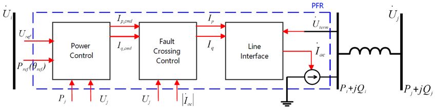
E3S Web of Conferences 257, 02031 (2021) https://doi.org/10.1051/e3sconf/202125702031
AESEE 2021
In the above references, the topological structure and 2 Modelling of PFR
model of PFR are different, but the function description of
the PFR in the power system is similar, that is, the network The architecture of PFR is shown in Figure 1, in which all
power flow hub integrating multiple system regulation and the incoming and outgoing lines are connected with the
protection functions. In this paper, based on the above common bus through the line power flow controller (PFC),
existing research on PFR, the steady-state and dynamic and each PFC automatically controls the corresponding
operation characteristics of PFR are studied, and the line power flow. In addition, some DC or frequency
corresponding mathematical model is established. Then, conversion equipment are connected to the common bus
the effect of PFR on optimizing the power flow and through voltage source converter (VSC). VSC controls the
improving the dynamic characteristics of distribution output and terminal voltage of corresponding equipment,
network is analysed by the case simulating. and it is also part of PFR.
Figure 1. Structure of PFR
The equivalent circuit of PFC is shown in Figure 2.
PFC is installed on the line connecting bus i and j, and has
three control parameters: the voltage amplitude VS and
phase angle ϕS at the series side and the current amplitude
Iq at the parallel side, which is orthogonal to bus voltage Figure 3. The equivalent circuit of VSC
Vi.
M 2 j 2 1 (2)
Vik e Vi
M1
Where, M1 and M2 are the modulation ratios of VSC1
and VSC2 respectively, and α1 and α2 are the phase shift
angles of VSC1 and VSC2 respectively.
From the above equivalent models, in the aspect of
Figure 2. The equivalent circuit of PFC power flow control, the PFC and VSC can be regarded as
phase-shifting transformers with controllable parameters.
According to the equivalent circuit and vector In addition, PFR may also include solid-state transformers
relationship, the basic mathematical relationship is as and various FACTS. Therefore, PFR can be equivalent to
follows: a combination of phase-shifting transformers, series
Vi ' Vi +VS voltage sources and parallel reactive power compensation.
Arg ( I q ) Arg (Vi ) / 2 (1)
Arg ( I S ) Arg (Vi ) 2.1 Steady-state model of PFR
'*
Re[V I ]
S i The steady-state model of PFR is mainly used to solve the
IS =
Vi optimal power flow (OPF). The OPF is to find the optimal
The VSC model is shown in Figure 3. The AC-DC-AC solution (system generator output, voltage amplitude and
conversion is realized by VSC1 and VSC2. If the bus phase angle) to meet the system constraints (voltage
voltage Vi is given, the voltage phase and amplitude of Vik constraints, power flow constraints, output constraints).
can be adjusted in a certain range based on the common The objective function can be composed of generation cost,
DC bus, so as to control the line power flow. network loss, transmission capacity and other indicators.
Taking minimization of network loss as an example, the
OPF model is as follows:
2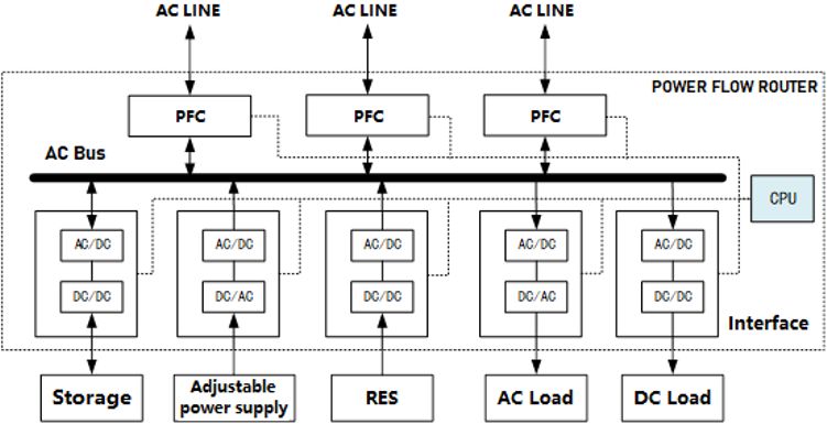
E3S Web of Conferences 257, 02031 (2021) https://doi.org/10.1051/e3sconf/202125702031
AESEE 2021
n
Where, ∆f is the difference between the objective
min Pb Vb V j (Gbj cos bj Bbj sin bj ) Pdb Psb
j 1 function value and the upper limit value.
n
(5) is introduced into the nonlinear indeterminate
Psi Pdi Vi V j (Gij cos ij Bij sin ij ) 0 (i 1,..., n) equations of augmented constrained power flow as shown
j 1 in (6). By using Newton Raphson method to solve (6), the
n optimal power flow with PFR can be obtained.
Qsi Qdi Vi V j (Gij sin ij Bij cos ij ) 0 (i 1,..., n) P P P P P P
j 1
yb
i j (Gij cos ij Bij sin ij ) tijVi Gij 0
Pij VV (k 1,..., l )
2
P Q Q Q Q Q Q
Q
i j (Gij cos ij Bij sin ij ) V j Gij / tij 0
Pji VV 2
(k 1,..., l ) f yb
f f f f f f yb
Vi min Vi Vi max (i 1,..., n)
yb
Psi min Psi Psi max (i 1,..., n) (6)
Qsi min Qsi Qsi max (i 1,..., n)
Where, α, β, δ are the auxiliary decision variables of V,
P and Q respectively, and yb is the auxiliary variable that
Pij min Pij Pij max (k 1,..., l ) transforms the objective function into the equation form.
(3)
Pji min Pji Pji max (k 1,..., l )
Where, P is the active power, Q is the reactive power, 2.2 Dynamic model of PFR
V is the voltage amplitude, θ is the voltage phase angle, G PFR is mainly used in power flow and voltage control, and
is the line conductance, B is the line susceptance, and t is stability control is its auxiliary function. In order to give
the non-standard transformation ratio. The subscript i full play to the role of PFR in enhancing system damping,
represents the ith node, ij represents the line between node stabilizing system oscillation and enhancing system
i and node j, s represents the input, d represents the output, reliability, it is necessary to study the impact of adding
and b represents the PCC point where the regional energy PFR device on system transient performance. Based on the
system connects to the superior power grid. steady-state power flow control, the control strategy of
If PFR is considered, t is regarded as a complex PFR in the transient process is formulated by using the
variable, characteristics of PFR to quickly adjust the active and
t t (4) reactive power of the transmission line.
According to the structure and working principle of
Then G and B are all variables of t . If t t t sin , (1) (2)
PFR, the transient stability model of PFR is shown in
where t (1) (tmax tmin ) / 2 , t (1) (tmax tmin ) / 2 , the G and B Figure 4. This model includes power control, fault
are variables of τ and σ. We can rewrite (3) as the crossing control and line interface. Among them, the
following partial differential equation: power control link controls the transmissing active and
Pi Gij Bij Gii reactive power of the line when the system is in normal
Vi [V j ( cos ij sin ij ) Vi ] operation. The fault crossing control link is the control
ij ij ij ij
Pi V [V ( Gij cos Bij sin ) V Gii ] logic when the system is subject to fault or large
i j
ij
ij
ij
ij i
ij disturbance. The line interface takes PFR as the controlled
ij current source and injects the calculated current into the
Q G B B
i
Vi [V j ( ij sin ij ij cos ij ) Vi ii ] line. The power control model and the fault crossing
ij ij ij ij
Q control model are shown in Figure 5 and Figure 6
Gij Bij B
i
Vi [V j ( sin ij cos ij ) Vi ii ] respectively.
ij ij ij ij
f G B G
Vb [V j ( bj cos bj bj sin bj ) Vb bb ]
bj bj bj bj
f Gbj Bbj G
Vb [V j ( cos bj sin bj ) Vb bb ]
bj bj
bj bj
Figure 4. The transient stability model of PFR
3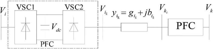
E3S Web of Conferences 257, 02031 (2021) https://doi.org/10.1051/e3sconf/202125702031
AESEE 2021
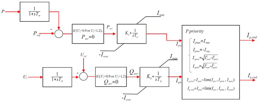
Figure 5. The power control model
Figure 6. The fault crossing control model
Where, Tm is the measuring time constant. Imax, Imin are are shown in Table 1 and Table 2.
maximum and minimum output current of converter
respectively. Kp, Tp are the scale factor and the integral
3.1 Steady state simulation analysis
time constant of active power control under normal
working conditions. Kq, Tq are the scale factor and the In the example system, PFR is installed on the central node
integral time constant of reactive power control under B2 of 220kV grid and the central node B13 of 110kV grid.
normal working conditions. Un is the rated voltage of PFR. The optimal power flow of the whole grid is solved, and
Kq_h and Kq_l are high voltage and low voltage forced the optimization objective is to minimize the network loss
reactive compensation coefficient respectively. Kpp is the of the whole grid, that is, to minimize the output of the
change rate of active current recovery. balance node G1. The comparison of calculation results is
shown in Table 3.
3 Case study
In order to verify the above models, the IEEE standard 5
machine 14 node calculation example system is used, and
the model structure is shown in Figure 7. The example
system has 5 generator nodes, among which G1 is the
balance node, G2, G3, G4 and G5 are PV nodes, and the
other 9 nodes are PQ nodes. The system consists of 20
branches, including 3 transformer branches. The node
parameters and branch parameters of the example system
4E3S Web of Conferences 257, 02031 (2021) https://doi.org/10.1051/e3sconf/202125702031
AESEE 2021
G G power flow of the system.
2 3
G
1 3.2 Transient simulation analysis
5 4
Transient simulation analysis focuses on the influence of
PFR on the transient stability limit of power system. In the
G
8 7
calculation, the dynamic model parameters of the
G generator, load and other equipment are selected from the
6
11 10
9
dynamic model parameters of the same capacity
12 equipment in the actual system, and the electromechanical
transient simulation is used. The simulation step length is
13 14
0.01s, and the calculation time is 20s. The triggering fault
Figure 7. The fault crossing control model of transient stability limit calculation is the N-1 fault of
interconnection line of the section between the external
Table 1. The node parameters of the example system grid and the regional system, and the time of fault
Pl Ql Pg Qg Vt occurrence is 1s.
No. Type
(p.u.) (p.u.) (p.u.) (p.u.) (p.u.)
1 Slack 0 0 0 0 1.06 The comparison of transient stability limit calculation
2 PV 0.217 0.127 0.4 0 1.045 results is shown in Table 4. Compared with the system
3 PV 0.942 0.19 0 0 1.01 without PFR, when PFR is installed in B2, the system load
4 PQ 0.478 -0.039 0 0 1 can be increased by 17.6MW, and the transient stability
5 PQ 0.076 0.016 0 0 1 limit of section power can be increased by 20.2MW. When
6 PV 0.112 0.075 0 0 1.07
7 PQ 0 0 0 0 1
PFR is installed in B2 and B13, the system load can be
8 PV 0 0 0 0 1.09 increased by 39.5MW, and the transient stability limit of
9 PQ 0.295 0.166 0 0 1 section power can be increased by 46.4MW. It can be seen
10 PQ 0.09 0.058 0 0 1 that the installation of PFR has a significant effect on
11 PQ 0.035 0.018 0 0 1 improving the load capacity and transient stability limit of
12 PQ 0.061 0.016 0 0 1
the system.
13 PQ 0.135 0.058 0 0 1
14 PQ 0.149 0.05 0 0 1
Table 4. Comparison of transient stability limit calculation
results
System Load Transient Stability
Table 2. The branch parameters of the example system No. Work
(MW) Limit (MW)
Connecting R X B 1 No PFR 268.6 243.3
No. Tk
nodes (p.u.) (p.u.) (p.u.)
2 PFR installed in B2 286.2 263.5
1 1-2 0.01938 0.05917 0.02640 1
PFR installed in
2 1-5 0.05403 0.22304 0.02460 1 3 308.1 289.7
B2 and B13
3 2-3 0.04699 0.19797 0.02190 1
4 2-4 0.05811 0.17632 0.0170 1
5 2-5 0.05695 017388 0.01730 1
Based on the limit power flow mode of the system
6 3-4 0.06701 0.17103 0.00640 1 without PFR, the transient stability of the system before
7 4-5 0.01335 0.04211 0.00000 1 and after PFR installation is compared, and the simulation
8 4-7 0.0000 0.20912 0.00000 0.978 results are shown in Figure 8.
9 4-9 0.0000 0.55618 0.00000 0.969
10 5-6 0.0000 0.25202 0.00000 0.932
11 6-11 0.09498 0.19890 0.00000 1
12 6-12 0.12291 0.25581 0.00000 1
13 6-13 0.06615 0.13027 0.00000 1
14 7-8 0.0000 0.17615 0.00000 1
15 7-9 0.0000 0.11001 0.00000 1
16 9-10 0.03181 0.08450 0.00000 1 a)
17 9-14 0.12711 0.27038 0.00000 1
18 10-11 0.08205 0.19207 0.00000 1
19 12-13 0.22092 0.19988 0.00000 1
20 13-14 0.17093 0.34802 0.00000 1
Table 3. Comparison of OPF calculating results
Output of G1 Network loss
No. Work b) c)
(p.u.) reduction rate
1 No OPF 2.4048 - Figure 8. The comparison of simulation results
2 OPF without PFR 2.3278 3.2% It can be seen from the simulation results that when the
3 OPF with PFR 2.1064 12.41% system is installed with PFR, the power angle stability and
voltage stability of the system are significantly improved
The results show that the network loss of the optimal when N-1 fault occurs in the section connecting line,
power flow can be reduced by 3.2% compared with that of which is the dual effect that PFR can adjust the active and
the conventional power flow. When PFR is installed in the reactive power injection of the line at the same time. The
system, the network loss can be further reduced, which is transmission power deviation of the section connecting
9.21% lower than the optimal power flow without PFR, line is significantly reduced compared with that without
i.e., the installed PFR has an obvious effect on the optimal PFR, so the stability of the system operation is improved.
5E3S Web of Conferences 257, 02031 (2021) https://doi.org/10.1051/e3sconf/202125702031
AESEE 2021
4 Conclusions Commun. (SmartGridComm'14), 43-48.
6. Lin Junhao, Li Victor O. K., Leung Ka-Cheong, Lam
Power flow router (PFR) has become an important Albert Y. S., 2017, "Optimal Power Flow with Power
element of energy Internet. It can solve the problem of Flow Routers", IEEE Transactions on Power Systems,
power flow control when a large number of distributed vol. 32, no. 1, 531-543.
generations and controllable loads are connected into the
grid. In this paper, the structure and operation principle of 7. CAO Yang, YUAN Liqiang, ZHU Shaomin, et al.,
PFR including the line power flow controller and the 2015, "Parameter Design of Energy Router Orienting
voltage source converter are studied, the steady-state Energy Internet", Power System Technology, vol. 39,
model of PFR based on the generalized inverse matrix no. 11, 3094-3101.
method for solving OPF is established, and the transient 8. Kado Yuichi, Shichijo Daiki, Deguchi Ikumi, Iwama
characteristics of PFR are studied. Based on the idea of Naoki, Kasashima Ryosuke, Wada Keiji, 2015,
modular modelling, the general transient model of PFR is "Power flow control of three-way isolated DC/DC
established, including power control part, fault crossing converter for Y-configuration power router", 2015
control part and line interface part. IEEE 2nd International Future Energy Electronics
The PFR model proposed in this paper provides an Conference, IFEEC 2015, 1-5.
effective method for power system simulation analysis 9. Kado Yuichi, Kasashima Ryosuke, Iwama Naoki,
with PFR. Next, further research work will be carried out Wada Keiji, 2016, "Implementation and performance
in the aspects of model improvement and actual power of three-way isolated DC/DC converter using SiC-
grid analysis, and the development of the PFR prototype MOSFETs for power flow control", 2016 IEEE 7th
will be guided. International Symposium on Power Electronics for
Distributed Generation Systems, PEDG 2016, 1-7.
Acknowledgment 10. GUO Hui, WANG Fei, ZHANG Lijun, LUO Jian,
2016, "Technologies of Energy Router-based Smart
Supported by the State Grid Corporation Headquarters Distributed Energy Network", Proceedings of the
Science and Technology Project (5204XQ190047) CSEE, vol. 36, no. 12, 3314-3324.
11. MIAO Jianqiang, ZHANG Ning, KANG Chongqing,
References 2017, "Analysis of the influence of energy routers on
the operation optimization of distribution network",
1. ZHAO Zhengming, FENG Gaohui, YUAN Proceedings of the CSEE, vol. 37, no. 10, 2832-2839.
Liqiang, ZHANG Chunpeng, 2017, "The 12. Weijie Dong, Lijuan Hu, Wanxing Sheng, et al., 2017,
Development and Key Technologies of Electric "Research on probabilistic optimal power flow of
Energy Router", Proceedings of the CSEE, vol. 37, no. distribution system with multilayer structure based on
13, 3823-3834. energy router", Journal of Engineering, vol. 2017, no.
2. Sánchez-Squella Antonio, Ortega Romeo, Griñó 13, 1621-1624.
Robert, Malo Shane, 2010, "Dynamic energy router: 13. TU Chunming, MENG Yang, XIAO Fan, LAN Zheng,
Energy management in electrical systems fed by SHUAI Zhikang, 2017, "An AC-DC Hybrid
multiple sources", IEEE Control Systems Magazine, Microgrid Energy Router and Operational Modal
vol. 30, no. 6, 72-80. Analysis", Transactions of China Electrotechnical
3. Behl Madhur, Aneja Mansimar, Jain Harsh, Society, vol. 32, no. 22, 176-188.
Mangharam Rahul, 2011, "EnRoute: An energy router 14. AI Xin, TAN Qian, LV Zhipeng, ZHANG Mingze,
for energy-efficient buildings", Proceedings of the 2018, "VSG with PBC Energy Router and Its
10th ACM/IEEE International Conference on Application in Microgrid", Journal of North China
Information Processing in Sensor Networks, IPSN'11, Electric Power University, vol. 45, no. 3, 1-9.
125-126. 15. Thomas James Jamal, Hernandez Jorge, Grijalva
4. Nguyen Phuong H., Kling Wil L., Ribeiro Paulo F., Santiago, 2013, "Power flow router sensititvities for
2011, "Agent-based power routing in Active post-contingency corrective control", 2013 IEEE
Distribution Networks", 2011 2nd IEEE PES Energy Conversion Congress and Exposition, ECCE
International Conference and Exhibition on 2013, 2590-2596.
Innovative Smart Grid Technologies, ISGT Europe 16. James Jamal Thomas, Jorge E. Hernandez, Santiago
2011, 1-6. Grijalva, 2014, "An investigation of the impact of
5. J. Lin, V. O. K. Li, K.-C. Leung, A. Y. S. Lam, 2014, dispatchable power routers on electricity markets and
“Architectural design and load flow study of power market participants", IEEE Power and Energy Society
flow routers,” Proc. IEEE Int. Conf. Smart Grid General Meeting, vol. 2014, no. 10, 1-5.
6You can also read