Impact of Satellite Elevation Mask in GPS+Galileo RTK Positioning - DLR
←
→
Page content transcription
If your browser does not render page correctly, please read the page content below
Impact of Satellite Elevation Mask in
                                      GPS+Galileo RTK Positioning
                                                           J. Manuel Castro-Arvizu∗ , Daniel Medina∗ , Ralf Ziebold∗
                                     ∗
                                         Institute of Communications and Navigation, German Aerospace Center (DLR), Germany

                                                                                  Abstract
                          Global Navigation Satellite Systems (GNSS) have become the keystone and main information supplier for
                      Positioning, Navigation and Timing (PNT) data. While providing an adequate open sky performance, the accuracy
                      of standard code-based GNSS techniques is insufficient for applications requiring precise navigation. Additionally,
                      GNSS positioning algorithms performance can be easily disturbed in signal-degraded environments due to space
                      weather events, obstacles, urban areas, bridges, limited open sky view and/or low-elevation multipath effects.
                      Hence, this study gives a comparative of the performance assessment for different high elevation masks of a
                      multi-frequency multi-GNSS RTK method in a loose combination (a pivot satellite is chosen for each constellation
                      and frequency) to avoid the case of the lack of coinciding frequencies and based in the code and carrier phase
                      measurements of the integration of multiple GNSS constellations. The analysis of the Ambiguity Dilution of
                      Precision (ADOP) and the number of fixed ratio epochs in both static and dynamic real scenarios, demonstrates
                      that the dual frequency L1/E1+L5/E5a GPS+Galileo RTK positioning solution approach presented in this study
                      has a good performance in terms of reliability, positioning accuracy and availability in comparative with a GPS-
                      only RTK algorithm when high elevation mask values are used.

             INTRODUCTION

             During recent years, the data fusion of multiple GNSS systems gives the possibility of having a better performance in
             Positioning, Velocity and Timing (PVT) solutions in terms of availability, accuracy and reliability in engineering and
             scientific applications [1–3]. Several GNSS-driven positioning solutions exist in literature and they are used depending
             of the data type, number of receivers, number of observation samples and user applications. This work is focused
             on Real Time Kinematic (RTK), a relative positioning procedure where the position of a receiver is determined with
             respect to a stationary base station of accurately known coordinates [4]. RTK uses double difference (DD) code
             and carrier phase measurements, eliminating atmospheric effects, clock offsets and both receiver/satellites biases
             obtaining a centimeter-level positioning accuracy.
                 The use of carrier phase observations is a main factor for precise navigation, since their noise is two orders of
             magnitude lower than code observations. However, carrier observations are ambiguous by an unknown number of
             integer ambiguities. The process of determining the integer ambiguities, denoted as Integer Ambiguity Resolution
             (IAR) [5], grants the estimation of precise positioning. The goal of IAR is to use the integer ambiguity constraints
             for the improvement of the navigation solution. The RTK functional model is generally expressed as a Least-squares
             (LS) adjustment, for which a closed-form solution does not exist. Thus, its minimization is resolved applying a three-
             steps decomposition. The first step, "float estimation", constitutes a LS procedure where the integer constraint on
             the ambiguities is discarded. Then, the IAR estimates the integer ambiguities based on the float solution. This
             stage is commonly solved applying the Least-squares AMBiguity Decorrelation Adjustment (LAMBDA) method
             [6, 7]. Finally, "solution fixing" realizes the enhancement on the position solution based on the estimated integer
             ambiguities.
                 GNSS-based positioning performance can be easily deteriorated during the navigation in urban scenarios, due
             to signal reflection and occlusion, limited open sky view and/or low-elevation multipath effects. Thus, the use of
             low-elevation satellites is limited in such signal-degraded scenarios. In the opposite side, the use of a high elevation
             mask carries a significant effect, since the geometry can deteriorate and the number of observations not be sufficient.
             These features drive to a poor performing IAR and thus a insufficiently positioning accuracy. However, when data
             fusion of multiple GNSS is used, the improvement of the IAR increases even when high elevation masks of satellites
             ares considered [2, 8, 9].

Proceedings of the 2020 International Technical Meeting,                              487                                         https://doi.org/10.33012/2020.17157
ION ITM 2020, San Diego, California, January 21-24, 2020
Hence, this study provides a performance assessment for different cut-off masks and a dual-frequency L1/L5 RTK
algorithm, configured in a loose combination to avoid the case of the lack of coinciding frequencies and based in the
code and carrier phase measurements of the integration of multiple GNSS constellations. The comparative between
combined GPS-Galileo and GPS-only performances is verified also.
    The importance of a good IAR results in a good positioning performance. One technique to measure the quality
of the IAR is the Ambiguity Dilution of Precision (ADOP) [10, 11]. ADOP gives a measure of the strength of the
IAR and the geometry of the ambiguities. ADOP has been studied in literature for GPS-only performance [12, 13]
and also for multiple GNSS systems [2, 11, 14] showing that when number of satellites increases, the ADOP has
better performance of ADOP assuring a prominent accuracy in terms of positioning.
    The remainder of the paper is organized as follows. The description of a GPS+Galileo measurement model in
a loose combination is given in Section Combined GPS+Galileo measurement model. The state space model and
technical description of the combined GPS+Galileo RTK positioning algorithm proposed in this work is depicted in
Section State Space Model for Float Solution. Section Fixed Solution: Ambiguity Resolution describes the technical
solution for the IAR and ADOP description. Section Ambiguity Resolution Analysis and Results illustrates results
with real data and Section Conclusions concludes the paper with final remarks.

COMBINED GPS+GALILEO MEASUREMENT MODEL

The main feature of RTK positioning technique is the simplification in the DD resolution of the phase integer
ambiguities. Figure 1 depicts a basic diagram of RTK technique. For every system there is a base satellite (Loose
combination). In the other hand where a base satellite is used for multiple systems is called tight combination
permitting double differentiating across different systems. This work is centered in a loose RTK implementation.

                                                         GNSS Constellation

                                                                  i-th satellite
                                             j-th satellite
                                             Base satellite

                                                        Φjr       Φir Φj           Φib
                                                                       b

                                                              r                b

                                          Rover Receiver                            Base Receiver

                 Figure 1: RTK Diagram where the base satellite is the pivot of one single system.

   The between receiver Single Difference (SD) observation is expressed as:

                                     ∆φir−b = ∆ρir−b + cδtr−b + λNr−b
                                                                  i
                                                                      + ir−b ,                                    (1)
                                       i
                                     ∆Cr−b    =    ∆ρir−b     + c∆tr−b +                  i
                                                                                         ξr−b ,                    (2)

where δtr−b is the clock bias for rover (r) and base (b) stations; c is the speed light; φ is the phase and C and code
measurements; ρ is the range between the satellite and receiver; N is the number of integer ambiguities; λ denotes
the wavelength at the corresponding frequency;  and ξ are the measurement noise for phase and code observations
respectively. The subprefix r − b means the difference between rover and base station according to the ith satellite.
   The respective DD equations where the receiver biases can be eliminated from Equations 1 and 2 according to

                                                                     488
Figure 1, finally can be expressed as:
∇∆φi−j i−j i−j i−j
r−b = ∇∆ρr−b + λ∇∆Nr−b + r−b , (3)
i−j i−j i−j
∇∆Cr−b = ∇∆ρr−b + ξr−b , (4)
where the subprefix i − j means the DD of code and phase of the ith satellites according to the j th base satellite.
Equations 3 and 4 are DD general expressions for one single-system only. However, for a a muti-GNSS case, several
pair of these equations exist for every system. Thus this study is focused in a RTK position solution using a combined
GPS+Galileo measurement set data, the general measurement subset vector DD observations for GPS-only (G)
system is:
∇∆φG = ∇∆ρG G G
r−b + λ∇∆Nr−b + r−b , (5)
G
∇∆C = ∇∆ρG
r−b + G
ξr−b (6)
Likewise for Galileo (E) system:
∇∆φE = ∇∆ρE E E
r−b + λ∇∆Nr−b + r−b , (7)
E
∇∆C = ∇∆ρE
r−b + E
ξr−b (8)
So when in Equation 6 and 8 the base satellite (pivot) changes in a single epoch, the inter-system bias is still
consistent and the continuous RTK positioning algorithm is still accomplished [15].
Two of the main features of a RTK algorithm
is obtaining a Float Solution and a Fixed Solution. Float solution
is referred as an Extended Kalman Filter x = p, v, NG , NE , where p is the XYZ-position vector, v is the XYZ-
velocity vector; NG is the SD float ambiguity vector of GPS and likewise NE is the SD float ambiguity vector of
Galileo.
STATE SPACE MODEL FOR FLOAT SOLUTION
The relation between code/phase measurements and position is defined as yk = ∇∆φG ∇∆φE ∇∆C G ∇∆C E =
hk (xk ) + νk , where yk ∈ R2n is the observation vector and corresponds to the code and phase double differences; the
observation error νk is assumed to be zero-mean normal-distributed of covariance Rk , and the nonlinear observation
function, hk (xk ),
∇∆ρG
r−b + λG D · NG
∇∆ρE + λE D · NE
hk = r−b , (9)
∇∆ρG r−b
∇∆ρE r−b
and the corresponding Jacobian used to solve the nonlinear filtering problem into an EKF solution is given by
derivatives δh
δxk is:
k
δ∇∆ρG
δp
r−b
0 λG DG 0 0 0
δ∇∆ρ E
δp
r−b
0 0 λE DE 0 0
Hk = . (10)
δ∇∆ρG
δp
r−b
0 0 0 0 0
E
δ∇∆ρr−b
δp 0 0 0 0 0
Notice that the measurement Jacobian matrix in (10) is evaluated at the predicted state to obtain a linear
formulation. In Equation 10, DG/E is the DD model for either GPS or Galileo. If there are mG common GPS
satellites, mE common Galileo satellites and the mth th
G and mE are the base satellite for GPS and Galileo respectively,
D , DmG −1×mG can be defined as DmG −1×mG = [−emG −1 , ImG −1×mG −1 ] for GPS system. Likewise DE ,
G
489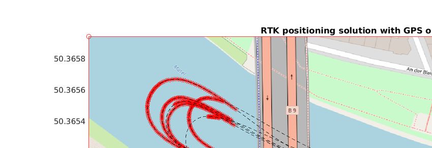
DmE −1×mE for Galileo system is expressed as DE , DmE −1×mE [15, 16]. Finally, for a combined GPS+Galileo
System, the D model is stated as:
I2×2 ⊗ DmG −1×mG 0mG −1×mE
D= (11)
0mE −1×mG I2×2 ⊗ DmE −1×mE
where emG/E is the mth
G/E column vector full of elements of 1. The full Kalman Filter algorithm can be written as
follows:
Algorithm 1: EKF formulation for float solution
Require: x̂0|0 , Px,0|0 , Qk and Rk , ∀ k
1: Set k ⇐ 1
Time update (prediction)
2: Estimate the predicted state:
x̂k|k−1 = Fx x̂k−1|k−1 .
3: Estimate the predicted error covariance:
Px,k|k−1 = Fx Px,k−1|k−1 F>
x + Qk .
Measurement update (estimation)
4: Estimate the predicted measurement:
ŷk|k−1 = hk x̂k|k−1 .
5: Estimate the innovation covariance matrix:
Py,k|k−1 = Hk Px,k|k−1 H>
k + Rk .
6: Estimate the Kalman gain
−1
K̃k = Px,k|k−1 H>
k Py,k|k−1 .
7: Estimate the updated state
x̂k|k = x̂k|k−1 + K̃k yk − ŷk|k−1 .
8: Estimate the corresponding error covariance:
Px,k|k = Px,k|k−1 − K̃k Gk Px,k|k−1 .
9: Set k ⇐ k + 1 and go to step 2.
where Px,k is the covariance matrix of the states at k th epoch; Px,k|k−1 is the one-step estimation of Pk ; K̃k is
the Kalman gain matrix; Fx one-step state transition matrix; Qk is the process noise covariance matrix and Rk is
the covariance matrix for the DD expressed as:
D · RφG · D
0 0 0
0 D · RφE · D 0 0
Rk = G
. (12)
0 0 D · RC ·D 0
E
0 0 0 D · RC · D
RC and Rφ are the code and carrier phase covariance measurement matrices respectively, whose characterization
is addressed in [17, 18].
FIXED SOLUTION: AMBIGUITY RESOLUTION
The Least-squares Ambiguity Decorrelation Adjustment (LAMBDA) algorithm [6] is considered for the process of in-
>
teger ambiguity resolution. After float solution implementation, from estimated state vector x̂k|k , N̂ = N̂G N̂E
and its respective PN,k|k taken from Px,k|k , are used as input for the Integer Least-square (ILS) LAMBDA estimator
>
to obtain the integer DD ambiguity N = NG NE . Then, the ratio-test upon the estimated ambiguities is
realized to decide whether to accept or not the integer solution [19, 20]. In this case, a fixed threshold Rthreshold of
3.0 [21] is considered:
>
Ñ = arg min N − N̂ · Q−1
N · N − N̂ , (13)
N
490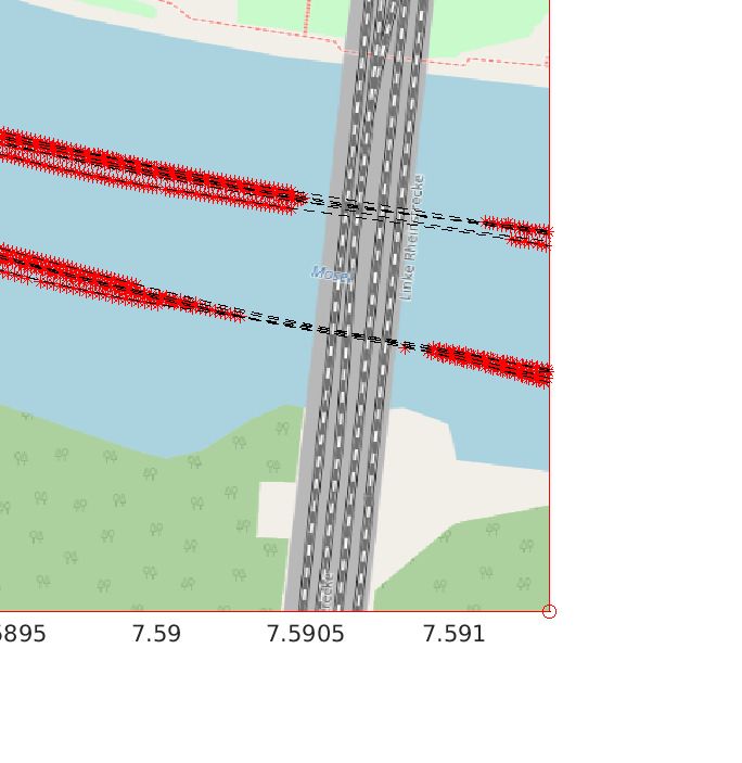
where QN is the variance-covariance matrix of float ambiguities and the fix ratio computation is:
                                                           >
                                                 Ñ2 − N̂· Q−1
                                                            N · Ñ2 − N̂
                                        R=           >                    .                                    (14)
                                             Ñ1 − N̂    · Q−1
                                                            N  ·   Ñ 1 − N̂

    From equation 14 if R > Rtreshhold , thus we have a fixed solution.
    As result, and easy way to compute the model strength of ambiguity resolution process is the ambiguity dilution
of precision (ADOP) [11, 12] which is given in cycles as:

                                                                  p       1

                                                   ADOP =          | QN | n                                        (15)

where n is the size ambiguity vector and | · | denotes the determinant. A successful ambiguity resolution is considered
when ADOP values is below a ADOPthreshold of 0.12 cycles corresponding an to Ambiguity Success Rate (ASR) of
99.9% [11].

AMBIGUITY RESOLUTION ANALYSIS AND RESULTS

In this section, the study and analysis of the impact of the elevation mask of satellites in IAR for a combined
GPS+Galileo RTK positioning solution are presented. As well, as the influence of a correct IAR in the position
solution.

Experimental Setup
The validation of the combined GPS+Galileo RTK position approach presented in study was validated with real
GNSS data recorded in a measurement campaign conducted in Koblenz, Germany in 2019 (DOYs 133 and 134). The
data was collected on board of the vessel MS Bingen at 1 Hz. The equipment consisted of a navXperience GNSS
antenna connected to a geodetic Javad DELTA Receiver and a TRIMBLE receiver for RTCM3 messages corrections
from the reference station with a ground truth known coordinates in Koblenz, Germany. Static data of DOY 133
(UTC 20:00 - 08:00) was used for the IAR analysis and the impact of the elevation mask of the combined GPS+Galileo
RTK position solution approach studied in this work. The validation was made with the comparative with single
frequency GPS-only System versus a Combined GPS+Galileo systems in dual frequency L1+L5 respectively.The
analysis in the performance of the RTK positioning algorithm in loose combination approach proposed in this study
was conducted for elevation masks of 10◦ , 15◦ , 25◦ , 35◦ and 45◦ respectively using the GNSS measurement data
of DOY 133. In order to track accurately the position of the vessel independently on the GNSS information, a
geodetic total station was placed on the shores of the river (see Figure 10) to ensure the availability of the reference
information even in areas where the GNSS performance was poor, as elaborated in [22].

Results and Analysis
Figure 2 gives a comparative of the number of satellites for both elevation masks of 10◦ and 45◦ . Its corresponding
ADOP values are shown in Figure 3 for a elevation mask of 10 and 45 respectively also. According to [7] and [11],
for a combined GPS+Galileo System, it is possible obtaining an ADOP value below 0.12 cycles and consequently
giving the certainty of a strong IAR a even for a high elevation mask in comparative with using a GPS-only system.
    The percentage of ADOP values below 0.12 cycles for different elevation mask is plotted in Figure 4. This figure
shows that, when the elevation mask increases, the percentage of ADOP values below of 0.12 cycles for a combined
GPS+Galileo system is significant in comparative with using a GPS-only System. Thus, a combined system will give
the certainty of an appropriate IAR and consequently an ASR of 99.9% even for high satellite elevation mask values.
    An empirical analysis of the fulfilment of the IAR method is the Success Fix solution ratio (FR) defined as:

                                                 Number of fixed solution
                                        FR =                              × 100                                    (16)
                                                 Number of total epochs

                                                                 491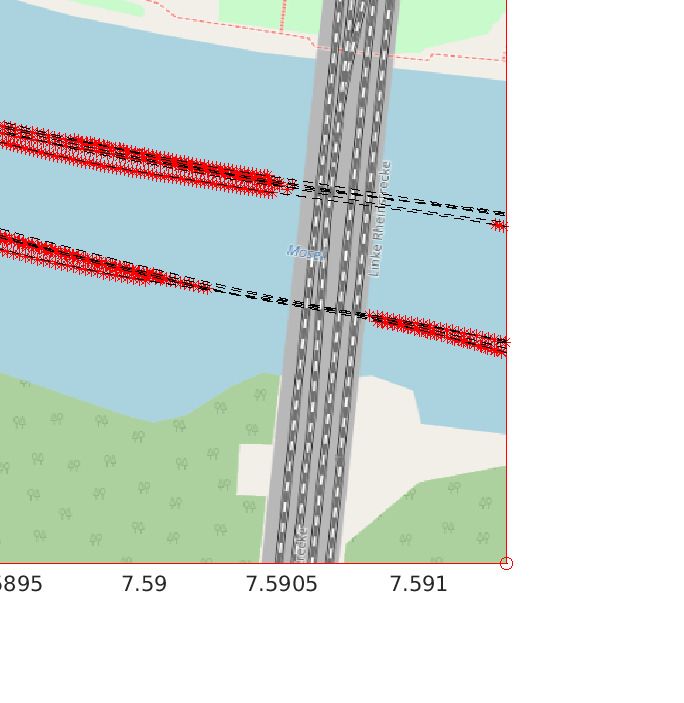
16

                        14

                        12
                                                                        GPS satellites
                                                                        GPS+Galileo Satellites
                        10

                         8

                         6
                             0    0.5   1      1.5     2         2.5    3            3.5            4
                                                                                                    10 4

                       0.5
                                                                                   ADOP G
                       14
                       0.4                                                         ADOP GE
                                                                                   ADOP threshold
                       0.3
                       12

                       0.2
                       10

                       0.1                                                  GPS satellites
                        8                                                   GPS+Galileo Satellites
                        16
                         0
                             0    0.5   1      1.5     2         2.5    3            3.5            4
                         6
                        14
                                                                                                    10 4

                         4
                        12
                             0    0.5   1      1.5     2         2.5    GPS satellites
                                                                        3            3.5             4
                                                                        GPS+Galileo Satellites
                        10                                                                          10 4

                         8
                       0.5
Figure 2: Number of GPS-only, GPS+Galileo satellites. ADOPTop
                                                           G
                                                                Figure corresponds to the analysis of an elevation
                       6   ◦
              mask of0.4 10
                         0   and
                               0.5the bottom
                                        1    figure
                                              1.5   to  the
                                                      ADOP
                                                       2   GE
                                                             analysis
                                                               2.5    of3 an elevation
                                                                                3.5    mask
                                                                                       4    of 45◦ .
                                                      ADOP threshold                                10 4
                       0.3
                         14
                       0.5

                       0.2                                                         ADOP G
                         12
                        0.4                                                        ADOP GE
                                                                                   ADOP threshold
                       0.1
                         10
                        0.3
                                                                            GPS satellites
                        08
                       0.2                                                  GPS+Galileo Satellites
                             0    0.5   1      1.5     2         2.5    3            3.5             4
                       0.1                                                                          10 4
                         6

                         0
                         40       0.5   1      1.5     2         2.5    3            3.5            4
                           0      0.5    1     1.5      2        2.5    3            3.5             4
                                                                                                    10 4
                                                                                                    10 4

                        0.5
                                                       ADOP G

                        0.4                            ADOP GE
                                                       ADOP threshold

                        0.3

                        0.2

                        0.1

                         0
                              0   0.5    1     1.5      2        2.5    3            3.5             4
                                                                                                    10 4

               Figure 3: Top Figure corresponds to ADOP values when an elevation mask of 10◦
  is se. As comparison, the bottom Figure plots the ADOP values when a high elevation mask of 45◦ is set.

                                                        492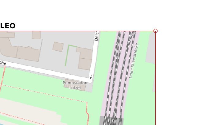
100
                                                                         GPS Galileo
                     90                                                  GPS

                     80

                     70

                     60

                     50

                     40

                     30

                     20

                     10

                      0
                               15             25               35             45
                                              Elevation Mask [°]

         Figure 4: Percentage of ADOP values below 0.12 cycles for different elevation masks values.

Figure 5: Success and unsuccessful fixed solutions with GPS-only and GPS+Galileo RTK positioning algorithm
                                           with elevation mask of 45◦

                                                     493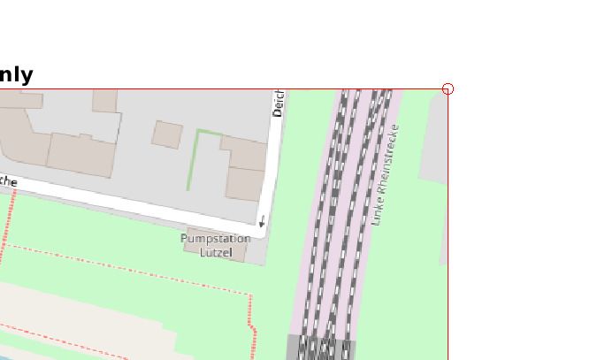
The comparative between the solution using a combined system and a GPS only system is depicted in Figure 5.
This Figure shows the percentage of Fixed solutions for a elevation mask of 45◦ . For a combined system, 82.41%
percentage of epochs have a fixed solution in contrast with a GPS-only system with only 25.24% of fixed solutions.
Table 1 numerically depicts and resumes the values for different elevation masks and its impact in the mean
ADOP, the percentage of ADOP values below 0.12 cycles and also the percentage of Success fixed solutions ratio.
From this table the best approach for a good combination of ADOP values and percentage of fixed solution ratio is
for a GPS+Galileo combined system when high satellite elevation mask are implicated.
10◦ 15◦ 25◦
System/F requency ADOP ADOP F R(%) ADOP ADOP F R(%) ADOP ADOP F R(%)
≤ ≤ ≤
0.12(%) 0.12(%) 0.12(%)
GP S L1 0.145 52.61 97.56 0.188 43.86 93.35 0.258 40.66 83.08
G + E L1/L5 0.086 99.95 100 0.125 98.94 99.18 0.135 85.02 98.80
35◦ 45◦
System/F requency ADOP %ADOP FR (%) ADOP ADOP F R(%)
≤ 0.12 ≤
0.12(%)
GP S L1 0.323 25.35 45.39 0.338 10.39 25.24
G + E L1/L5 0.144 67.64 97.14 0.154 28.36 82.41
Table 1: Mean ADOP, Percentage of ADOP values below 0.12 cycles and Success Fix solution ratio (FR), for
different elevation masks for a GPS-only (G) System or a combined GPS+Galileo (G+E) System.
Figures 6 and7 illustrates the impact of a high elevation mask of 45◦ in the positioning performance with a
combined GPS+Galileo system in comparative with a GPS-only system. These Figures exhibit the horizontal and
vertical error as well as the number of satellites. The mean horizontal and vertical error for a combined GPS+Galileo
system are 0.0258 meters and 0.0111 meters respectively. The mean errors are lower in contrast with a GPS-only
system with a mean horizontal error of 0.0359 meters and a mean vertical error of 0.0135 meters.
Finally, with the GNSS measurement data acquired in DOY 134 and with an elevation mask of 35◦ , a dynamical
and urban scenario was taken into account as a second validation. An elevation mask of 35◦ . The difference in the
number of fixed solutions of a GPS-only System with respect to a combined GPS+Galileo RTK positioning algorithm
approach is depicted in Figure 8.
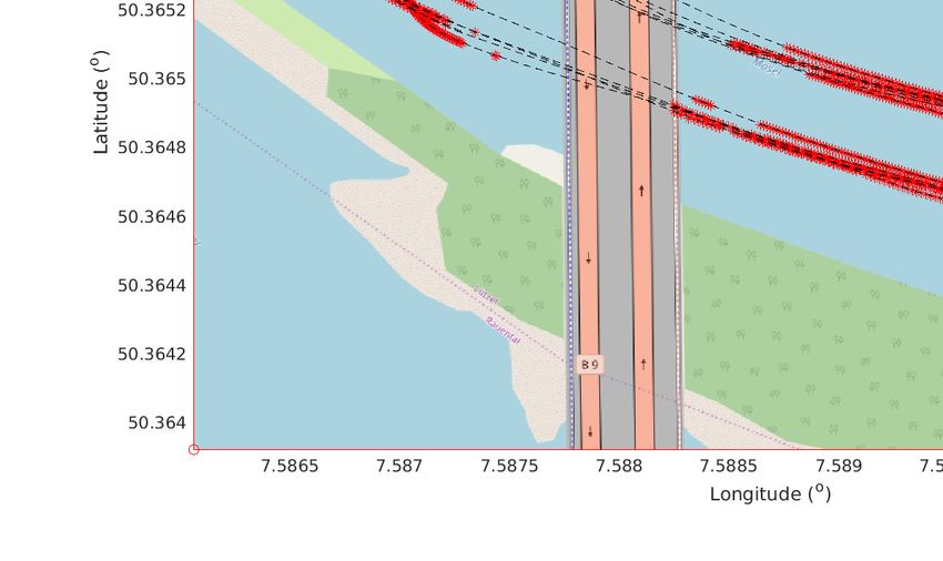
Figures 9 and 10 illustrate the comparative of fixed solutions between a GPS-only system with respect to a
combined GPS+Galileo system. The fixed solutions in this a dynamical scenario are contrasted with a reference tra-
jectory. Figure 8 also exhibits that the number of fixed solutions is superior in a 41.32% for a combined GPS+Galileo
System when a high elevation mask is set with respect to a GPS-only System.
CONCLUSIONS
With a Galileo System scheduled with a full operational capability in 2020 and with modernized GPS satellites with L5
frequency available, GNSS positioning solutions open the opportunity to the data fusion of multiple satellite systems
and also dual-frequency. This study has formulated the benefits under high elevation masks of a dual-frequency
combined GPS+ Galileo RTK positioning algorithm approach accounting for realistic conditions. The analysis and
study of the ADOP for high satellite elevation mask was presented. This study shows that even with a low elevation
mask of 10◦ , a GPS-only System offers a 52.61% of the mean ASR in comparative with a combined dual-System that
offer 99.95% of the mean ASR. This performance is comparable even with a elevation mask of 45◦ when a combined
GPS+Galileo System offers a benefit of 57.17% of the mean ASR with respect to GPS-only System. This efficiency
gives an evidence of a strong IAR and by consequence a better position solution approach. This remark is also
verified with the percentage of Success fixed solutions where a combined GPS+Galileo-System gives a prominent
performance. The validation of this work is significant when environmental constraints are considerable an a high
elevation mask is set.
494
GPS-only with elevation mask 45°
                          0.1

                         0.05

                            0
                                0   0.5      1      1.5       2        2.5      3   3.5    4
                                                                                          10 4
                         0.06

                         0.04

                         0.02

                            0
                                0   0.5      1      1.5       2        2.5      3   3.5    4
                                                                                          10 4
                            8

                            7

                            6

                            5
                                0   0.5      1      1.5       2        2.5      3   3.5    4
                                                                                          10 4

Figure 6: Horizontal and Vertical error for GPS-only RTK positioning solution. Only fixed solutions are considered
                                                 in this analysis

                                          GPS+Galileo with elevation mask 45°
                          0.1

                         0.05

                            0
                                0   0.5      1      1.5       2        2.5      3   3.5    4
                                                                                          10 4
                         0.04

                         0.02

                            0
                                0   0.5      1      1.5       2        2.5      3   3.5    4
                                                                                          10 4
                           14

                           12

                           10

                            8
                                0   0.5      1      1.5       2        2.5      3   3.5    4
                                                                                          10 4

    Figure 7: Horizontal and Vertical error for a combined GPS+Galileo RTK positioning solution. Only fixed
                                     solutions are considered in this analysis

                                                             495
Fixed Solutions with GPS + Galileo
1.5
GPS/Galileo Fixed Solution 85.21%
succes/unsucces
1
0.5
0
0 500 1000 1500 2000 2500 3000 3500 4000 4500 5000
samples
Fixed Solutions with GPS only
1.5
GPS Fixed Solution 43.89%
succes/unsucces
1
0.5
0
0 500 1000 1500 2000 2500 3000 3500 4000 4500 5000
samples
Figure 8: Success and unsuccessful fixed solutions in a dynamical scenario.
Figure 9: Fixed solutions using a GPS-only RTK positioning algorithm in a dynamical scenario.
496Figure 10: Fixed solutions using a combined GPS+Galileo RTK positioning algorithm in a dynamical scenario.
REFERENCES
[1] Tuan Li, Hongping Zhang, Xiaoji Niu, and Zhouzheng Gao. Tightly-coupled integration of multi-gnss single-frequency RTK and
MEMS-IMU for enhanced positioning performance. Sensors (Switzerland), 17(11), 2017.
[2] Kan Wang, Pei Chen, and Peter J.G. Teunissen. Single-epoch, single-frequency multi-GNSS l5 RTK under high-elevation masking.
Sensors (Switzerland), 19(5):1–21, 2019.
[3] Daniel Medina, Anja Heßelbarth, Rauno Büscher, Ralf Ziebold, and Jesús García. On the Kalman filtering formulation for RTK joint
positioning and attitude quaternion determination. In 2018 IEEE/ION Position, Location and Navigation Symposium (PLANS),
pages 597–604. IEEE, 2018.
[4] Richard B Langley. Rtk Gps. GPS World, pages 70–75, 1998.
[5] D. Montello and A Maglie Larghe. Least-Squares Estimation of the Integer GPS Ambiguities. (August), 1993.
[6] P. J. G. Teunissen, P. J. de Jonge, and Christian C. C. J. M. Tiberius. The LAMBDA-Method for Fast GPS Surveying. Proceedings
of International Symposium «GPS technology applications»’, (1):203–210, 1995.
[7] P. J.G. Teunissen, R. Odolinski, and D. Odijk. Instantaneous BeiDou+GPS RTK positioning with high cut-off elevation angles.
Journal of Geodesy, 2014.
[8] PJG Teunissen, Robert Odolinski, and Dennis Odijk. Instantaneous BeiDou+ GPS RTK positioning with high cut-off elevation
angles. Journal of geodesy, 88(4):335–350, 2014.
[9] Robert Odolinski, Peter JG Teunissen, and Dennis Odijk. Combined BDS, Galileo, QZSS and GPS single-frequency RTK. GPS
solutions, 19(1):151–163, 2015.
[10] P. J.G. Teunissen. A canonical theory for short GPS baselines. Part IV: Precision versus reliability. Journal of Geodesy, 1997.
[11] D. Odijk and P. J G Teunissen. ADOP in closed form for a hierarchy of multi-frequency single-baseline GNSS models. Journal of
Geodesy, 82(8):473–492, 2008.
[12] Peter J G Teunissen and Dennis Odijk. Ambiguity dilution of precision: Definition, properties and application. Proceedings of ION
GPS, 1(October):891–899, 1997.
[13] Bruno M Scherzinger, Applanix Corporation, and Richmond Hill. Precise Robust Positioning with Inertial / GPS RTK. System,
pages 155–162, 1983.
[14] Björn Reuper, Matthias Becker, and Stefan Leinen. Benefits of multi-constellation/multi-frequency GNSS in a tightly coupled
GNSS/IMU/Odometry integration algorithm. Sensors (Switzerland), 18(9):1–25, 2018.
[15] Wang Gao, Xiaolin Meng, Chengfa Gao, Shuguo Pan, and Denghui Wang. Combined GPS and BDS for single-frequency continuous
497RTK positioning through real-time estimation of differential inter-system biases. GPS Solutions, 22(1):1–13, 2018.
[16] Daniel Medina, Vincenzo Centrone, Ralf Ziebold, and Jesús García. Attitude Determination via GNSS Carrier Phase and Inertial
Aiding. In ION GNSS+, The International Technical Meeting of the Satellite Division of The Institute of Navigation, Miami, FL,
Sep 2019.
[17] R Odolinski, Peter Teunissen, and Dennis Odijk. An analysis of combined COMPASS/BeiDou-2 and GPS single-and multiple-
frequency RTK positioning. In Proceedings of the ION 2013 Pacific PNT Meeting, pages 69–90. INST NAVIGATION, 2013.
[18] Daniel Medina, Kasia Gibson, Ralf Ziebold, and Pau Closas. Determination of Pseudorange Error Models and Multipath Charac-
terization under Signal-Degraded Scenarios. In PROCEEDINGS OF ION GNSS+. Institute of Navigation, 2018.
[19] Peter JG Teunissen and Sandra Verhagen. The GNSS ambiguity ratio-test revisited: a better way of using it. Survey Review,
41(312):138–151, 2009.
[20] Sandra Verhagen and Peter JG Teunissen. The ratio test for future GNSS ambiguity resolution. GPS solutions, 17(4):535–548, 2013.
[21] Ying Xu and Wu Chen. Performance analysis of GPS/BDS dual/triple-frequency network RTK in urban areas: A case study in
Hong Kong. Sensors (Switzerland), 18(8), 2018.
[22] Daniel Arias Medina, Michailas Romanovas, Iván Herrera-Pinzón, and Ralf Ziebold. Robust position and velocity estimation methods
in integrated navigation systems for inland water applications. In 2016 IEEE/ION Position, Location and Navigation Symposium
(PLANS), pages 491–501. IEEE, 2016.
498You can also read