National Greenhouse Gas Inventory for Thailand's Second National Communication and Mitigation Aspects

IPCC Expert Meeting: Application of the 2006 IPCC Guidelines to Other Areas
 1-3 July 2014, Sofia, Bulgaria

 National Greenhouse Gas Inventory for
Thailand’s Second National Communication and
 Mitigation Aspects

 Jakapong Pongthanaisawan, PhD
 Senior Policy Researcher
 National Science Technology and Innovation Policy Office
 Ministry of Science and Technology, Thailand

Outline
• History of Thailand’s National GHG Inventory
• Second National Communication (SNC) and
 National GHG Inventory
• Mitigation Assessment
  National Level – Energy Sector
  Subsector Level – Road Transport Sector
• Conclusion and Recommendation

 2

History of Thailand’s National GHG Inventory

 1st National GHG Inventory
 • As a part of Thailand’s Initial
 National Communication (INC)
 • Using the Revised 1996 IPCC
 Guidelines to estimate the
 emissions in 1994
 • Prepared by Office of
 Environmental Policy and
 Planning (OEPP), Ministry of
 Science and Technology
 (MOST)
 • Submitted to UNFCCC on
 November 13, 2000

 3

History of Thailand’s National GHG Inventory

 2nd National GHG Inventory
 • As a part of Thailand’s Second
 National Communication (SNC)
 • Followed the guidelines:
 – Revised 1996 IPCC Guidelines to
 estimate the emissions
 – 2000 IPCC Good Practice Guidance
 and Uncertainty Management in
 Nation Greenhouse Gas Inventories
 – 2003 Good Practice Guidance for
 Land Use, Land-use Change and
 Forestry
 • Prepared by Office of Natural
 Resources and Environmental
 Policy and Planning (ONEP),
 Ministry of Natural Resources and
 Environment (MORE)
 • Submitted to UNFCCC on March 24,
 2011
 4

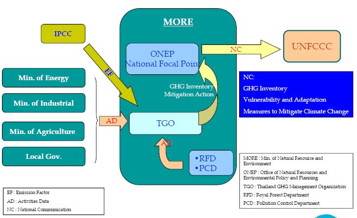
SNC and National GHG Inventory
 Institutional Framework of SNC

 Source: TGO 5

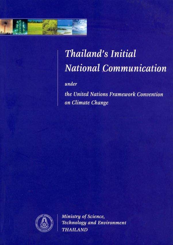
Structure of SNC Organization

 JGSEE – the Joint Graduate School of Energy and Environment, King Mongkut’s University of Technology Thonburi
 CU – Chulalongkorn University

 Source: JGSEE, KMUTT 6

Conceptual Framework of National GHG Inventory

 Guideline
 1. Revised 1996 IPCC
 Guidelines for National
 Greenhouse Gas Inventories
 2. 2000 IPCC Good Practice
 Guidance and Uncertainty
 Management in National
 Greenhouse Gas Inventories
 3. 2003 Good Practice
 Guidance for Land Use,
 Land-Use Change and
 Forestry
DEDE = Department of Alternative Energy Development and Efficiency
EGAT = Electricity Generating Authority of Thailand
PTT = Petroleum Authority of Thailand OTP= Office of Transport and Traffic Policy and Planning
EPPO = Energy Policy and Planning Office DIW = Department of Industrial Work
DLD = Department of Land Development OAC = Office of Agriculture Economics
RFD = Royal Forest Department BMA= Bangkok Metropolitan Administrative
PCD = Pollution Control Department

Source: Thailand’s Second National Communication 7

Framework of GHG Inventory Methodology

 Type of GHG
 Carbon Dioxide: CO2
 Methane: CH4
 Nitrous Oxide: N2O
 Hydrofluorocarbon: HFC
 Perfluorocarbon: PFC
 Sulfur Hexafluoride: SF6

Source: Thailand’s Second National Communication 8

Total GHG Emission

 =229.08 Mt CO2eq

 Source: Thailand’s Second National Communication
 9

GHG Emission from Energy Sector
 Emission in 2000 by 'Energy Sector' (Mt CO2 eq, %)
 Waste, 9.32, 4.1% 1A2 Manufacturing
 industries and
 LULUCF, -7.90, -3.4% construction, 30.78,
 19.3%
 1A1 Energy
 Industries, 66.44,
 41.7%
 Agriculture,
 Energy, 159.39,
 51.88, 22.6%
 69.6%
 1A3 Transport,
 1B2 Oil and natural 44.70, 28.0%
 gas, 4.56, 2.9%
 Industrial processes, 1A4b Residential,
 16.39, 7.2% 1B1 Solid fuels, 0.67, 1A4c 5.58, 3.5%
 0.4% Agriculture/Forestry/
 Total GHG Emission with LULUCF = 229.08 MtEq Fishing, 6.67, 4.2%

Source: Thailand’s Second National Communication
 10

Mitigation Assessment :
National Level

Mitigation Assessment : National Level
Concept, Structure and Steps

 1. Collect data.
 2. Assemble base year/historical data on
 activities, technologies, practices and
 emission factors.
 3. Calibrate base year to standardized
 statistics such as national energy
 balance or emissions inventory.
 4. Prepare baseline scenario(s).
 5. Screen mitigation options.
 6. Prepare mitigation scenario(s) and
 sensitivity analyses.
 7. Assess impacts (social, economic,
 environmental).
 8. Develop Mitigation Strategy.
 9. Prepare reports.

Source: Module2 mitigation concept, UNFCCC
 12

Estimation of GHG Emission
Methodology
 Macroeconomic – Econometric Model
 AD = f (GDP, Pop, Price, Irrigation Area,
 Default EF from 2006 IPCC
 Crop Area, etc.) Guideline

 = ∙ 
 E = Emissions or Removals
 AD = Activity Data - data of a human activity resulting in emissions or removals
 EF = Emission Factor - coefficients which quantify the emissions or removals
 per unit activity

 Sectors
 Energy, Industrial Processes and Product Use (IPPU), Agriculture, Forestry and
 Other Land Use (AFOLU), and Waste
 13

Scenario Analysis
• Baseline Scenario (Business-as-usual)
 – Socio-economic Assumptions
 • Population growth rate
 • GDP growth rate
 • Irrigation area
 • Crop area, etc.
• Mitigation Scenario (Energy Sector)
 – Electricity Generation
 • Promotion of technologies for electricity generation from renewable
 energy and low-carbon fossil fuel
 • Improve efficiency of generation and transmission system
 – End-use Sectors
 • Introduction of high energy efficiency technology and renewable
 energy for heat in industrial sector, building sector and transport
 sector.

 14

Mitigation Scenario
Screening Cost Curve for Mitigation Technology Selection
 Priority

 - Ton of CO2 Avoided
 - Cost of Saved Carbon ($/tCO2)

Criteria
• Potential for large impact on greenhouse gases (GHGs)
• Consistency with national development goals
• Consistency with national environmental goals
• Potential effectiveness of implementation policies
• Sustainability of an option
• Data availability for evaluation
• Institutional considerations 15

Mitigation Scenario – Energy Sector

 16

GHG Emission Projection – BAU Scenario

 Mt of CO2eq
 Sector 2010 2020 2030 2040 2050
 Energy 211.5 315.5 463.6 687.2 1036.9
 IPPU 32 57.1 96.1 106 120.7
 AFOLU 88.1 109.4 135 166.8 208.1
 Waste 13.8 16.6 20.4 25.7 33.1
 Total 345.4 498.6 715.1 985.7 1398.8

Assumptions: average GDP growth rate ~4% per year (NESDB, 2008) 17

GHG Emission Mitigation

 Mt of CO2-eq
 2010 2020 2030 2040 2050
 BAU 0 0 0 0 0
 Electricity Generation -1.4 -38.6 -107.7 -161.6 -239.9
 Industry -0.3 -5.3 -5.5 -5.8 -6.4
 Building -4.5 -14.2 -24.4 -26.6 -28.7
 Transport -1.5 -4.9 -8.4 -9.6 -10.8
 Total -7.7 -63.0 -146.0 -203.6 -285.8
 % Reduction -2.2% -12.6% -20.4% -20.7% -20.4% 18

Mitigation Assessment :
Road Transport Sector

Mitigation Assessment : Road Transport Sector
20-Year Energy Efficiency Development Plan (EEDP 2011-2030)
 Target: reducing “energy intensity”
 (the amount of energy used per unit of
 GDP) by 25% by 2030 compared with
 2005 as base year, accounting for total
 energy saving of 30,000 kilotons of oil
 equivalent (ktoe) in 2030

 Energy saving targets by sector
 Energy
 Sector Saving % share
 (ktoe)
 Transportation 13,400 44.7%
 Industry 11,300 37.7%
 Large Commercial Building 2,300 7.6%
 Small Commercial Building
 & Residential 3,000 10.0%

 Source: Energy Policy and Planning Office (2011) 20

Mitigation Assessment : Road Transport Sector
10-Year Alternative Energy Development Plan (AEDP 2012-2021)

 Target: using 25% of
 renewable energy for total
 energy consumption (heat
 and electricity generation)
 by the year 2021

 Note: MW=Megawatt
 ktoe = kilotons of oil equivalent
 ML = Million liters

Source: Department of Alternative Energy Development and Efficiency (2012)
 21

Energy Policies in Thailand
• Alternative Energy Development Plan • Energy Efficiency Development Plan
 (2012-2021) (2011-2030)
 – Switch conventional fossil fuel, – Promotion of high energy
 such as gasoline and diesel, to efficiency vehicle technologies
 biofuels, i.e. bioethanol and for private vehicles, such as eco-
 biodiesel car, hybrid car and electric
 vehicle

 22

Overview of Methodology

 End-Use Energy Demand Model Legend:
 Exogenous Inputs
 Scenarios Analysis: Vehicle Sale by Vehicle Type [Vehicles]
 Alternative Vehicle Stocks by Vehicle Type Model Calculations
 Fuel Share of Vehicle Sale by Fuel Type [%]
 Technology Options Survival Rate of Vehicle by Age [%] [Vehicles]
 Final Outputs

 Vehicle Stock Profile by Age [%]

 Technology Penetration [%]
 Annual Average VKT by Total VKT by Vehicle Type
 Fuel Share of Vehicle Sale [%] Stock Average VKT by
 Vehicle Type [km/year]
 % Share of Alternative Fuels [%] Vehicle Type [Veh-km] [Vehicle-kilometer]
Fuel Economy of Vehicle [km/liter]
 VKT Degradation by Age [%] Calibration and
 Verification
 On-Road Fuel Economy by Stock Average Fuel
 Vehicle and Fuel Type [km/liter] End-use Energy Consumption
 Economy by Vehicle
 Fuel Economy Degradation by [MJ]
 Age [%] and Fuel Type [km/liter]

 Tank-to-Wheel GHG Emission Factors Tank-to-Wheel GHG Emissions GHG Emissions Estimation
 [kg/MJ] [kg]

 Well-to-Tank GHG Emission Factors Life Cycle GHG
 [kg/MJ]
 Well-to-Tank GHG Emissions [kg]
 Emissions [kg]

 23

End-use Energy Demand Model
 ( ) = , , ( ) × , , ( ) × − 
 , , ( )
 
 Where ( ) is the total energy demand in a calendar year t (MJ)
 , , ( ) is the total stock of vehicle type i , which use fuel type j, in a
 calendar year t (vehicles)
 , , ( ) is the stock’s average annual vehicle kilometer of travel of
 a given vehicle type i, which use fuel type j, in a calendar year t (kilometers)
 , , ( ) is the stock’s average fuel economy of that given vehicle type i,
 which use fuel type j, in a calendar year t (vehicle-kilometer per MJ)
 t is the calendar year of consideration for a vehicle stock estimation
 i is the type of vehicles
 j is the type of fuels.

 24

• Stock Turnover Analysis
 = 

 , , ( ) = , ( ) × × , ( )
 = ′

 Where , , ( ) is the number of vehicle stock type i which use fuel type j in a calendar year t
 (vehicles)
 , ( ) is the number of new vehicle type i that sold in vintage year v (vehicles)
 , ( ) is the number of new vehicle type i that sold in vintage year v (vehicles)
 is the survival rate of vehicles type i with age k (%)
 , ( ) is the percentage share of fuel type j within the sales of vehicle type i in
 the vintage year v (%)
 v is the vintage year of vehicles, of which v < t
 v’ is the oldest vintage year of vehicles in the stock.
 k is the age of vehicle, where k = t – v (years)

 25

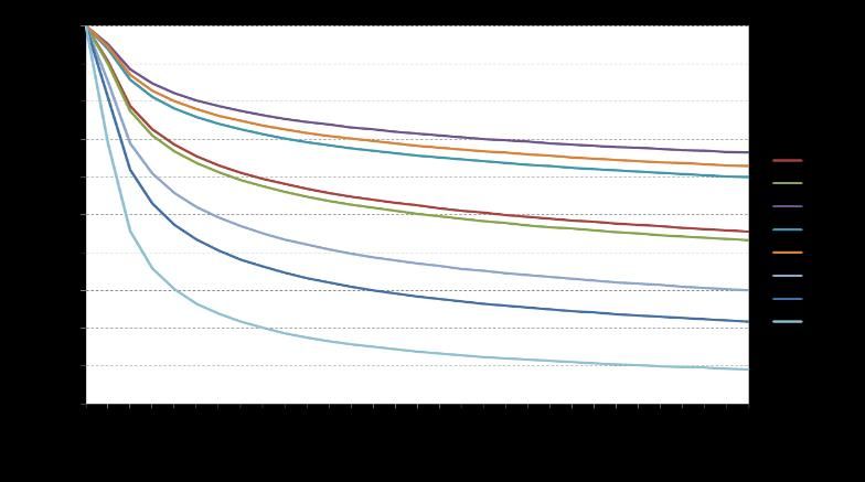
 Survival Rate of Vehicles ( )
 • Survival rate of vehicles is a probability that vehicles are survived with
 increasing ages after they entered the market.
 
 Observed data + 
 Weibull Function = − , ≡ 
 Modified Weibull Function 

 Where is the survival rate of vehicle
 type i with age k
 k is the age of vehicles
 bi is the failure steepness for vehicles
 type i (bi>1, i.e. failure rate increase
 with age)
 Ti is the characteristic service life for
S-shaped Gompertz scrapping curve vehicle type i.

 Data sources: Department of Land Transport (DLT)
 26

Age
 PC PU TAXI COMC 3WL MC BUS TRK
(Years)
 bi 4.02 2.04 7623.24 2.66 2.22 2.18 2.80 2.22
 Ti 39.70 55.17 7634.32 18.09 15.68 15.42 24.46 30.05
 R2 0.79 0.91 0.94 0.77 0.90 0.97 0.84 0.8427

 , ( ) = , , 
 Where , and , are coefficients of variable k (vehicle
 age) of vehicle type i which uses fuel type j.

 ℎ, , = , × ℎ, , 0
 = , , × ℎ, , (0)

 Where , ( ) is the degradation factor of VKT of vehicle type i

 = 
 which use fuel type j with age k
 = ′ , , , × ℎ, , 
 , , ( ) = ℎ, , ( ) is the annual average VKT of vehicle type i
 , , ( )
 which use fuel type j with age k (kilometers)
 Where , , ( ) is the stock’s annual average vehicle
 ℎ, , (0) is the annual average VKT of new vehicle
 kilometer of travel of vehicles type i which use fuel type j
 type i which use fuel type j (kilometers)
 in a calendar year t (kilometers per vehicle)
 , and , are coefficients of variable k (vehicle age) of
 , ( , ) is the number of vehicle type i that sold in
 vehicle type i which use fuel type j.
 vintage year v, which still remains on road in a calendar
 year t (vehicles)
 Data sources: King Mongkut’s Institute of Technology Thonburi (KMITT)
 28

Vehicle Type PC PU TAXI COMC 3WL MC BUS TRK
VKT of New Vehicle
 23,248 37,955 72,154 26,758 13,766 14,690 98,395 98,111
 (km/year)
 αi 0.907 0.900 0.953 0.939 0.946 0.853 0.811 0.689
 βi -0.202 -0.215 -0.106 -0.132 -0.120 -0.307 -0.387 -0.594
 29
 R2 0.98 0.98 0.99 0.99 0.99 0.98 0.98 0.97

 Fuel Economy of Vehicles ( , , ( ))
• Fuel economy is an average vehicle-
 distance travelled per unit of fuel Fuel Economy
 Vehicle
 used. It is generally presented in term (Vehicle-kilometer per liter)
 Type
 of vehicle-kilometer per liter. Gasoline Diesel LPG CNG*
• The efficiency of a vehicle is normally PC 12.27 11.31 10.69 10.86
 reducing when the vehicle get older. PU 11.82 11.93 11.06 10.78
• According to a survey data of KMITT,
 TAXI 13.50 10.00 9.66 11.16
 relationship between the degradation
 of vehicle efficiency and its age could COMC 9.37 8.34 11.22 8.71
 not be found. 3WL 17.68 15.37 10.80 10.25
• Therefore, in this study, we assumed MC 28.71 - - -
 that age of vehicle does not affect to BUS - 3.91 - 2.26
 the fuel economy of vehicles. The fuel
 TRK - 4.14 - 1.67
 economy of vehicles was also assumed
 to be constant. Note: * Unit of CNG fuel economy is veh-km per kg.

 Data sources: King Mongkut’s Institute of Technology Thonburi (KMITT) and
 Energy Policy and Planning Office (EPPO)
 30

GHG Emissions Estimation
 Non-CO2 Emissions
• Default GHG Emission Factors
 4 = × 4, 
 CO2 Emission
 2 = × , 2 = × 2 , 

 Where 2 is the carbon dioxide emission (t CO2) Where 4 is the methane emission (kg)
 is the fuel consumption of fuel type j (ktoe) 2 is the nitrous oxide emission (kg)
 4, is the methane emission factor
 , is the carbon emission factor of fuel type j (t C/TJ)
 of fuel type j (kg/TJ)
 2 , is the nitrous oxide emission
 factor of fuel type j (kg/TJ).

 31

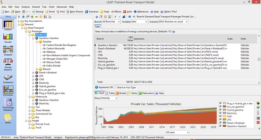
Long-range Energy Alternatives Planning (LEAP) System

 32

Life Cycle of Fuel Supply-Demand of Road Transport Sector

• Well-to-Wheel Analysis for Transport Fuel Systems
 – Well-to-Tank: Fuel Production
 – Tank-to-Wheel: Fuel Utilization

 Well-to-Tank Tank-to-Wheel

 Well-to-Wheel

 33

Supply Chain of Road Transport Fuels
 Storage/ Storage/
 Primary Energy Transport
 Conversion Distribution
 Final Energy

- Palm plantation, cultivation,
 and transportation Storage/ Production of Storage/
- Crude Palm Oil Extraction
 Crude Palm Oil
 Transport Biodiesel Distribution Biodiesel
- Palm Oil Production

- Sugar cane farming, cultivation
 and transportation Storage/ Production of Storage/
- Sugar Production
 Molasses
 Transport Bioethanol Distribution Bioethanol
 (Molasses as by product)

 Diesel
 Refining to
 Crude Oil Extraction and Storage/ Storage/
 Transportation
 Crude Oil
 Transport
 Gasoline/Diesel/ Distribution Gasoline
 LPG/Fuel Oil
 LPG
 Natural Gas Extraction and Seperation/
 Natural Gas Storage/
 Transportation
 Transport Purifying

 Diesel/Fuel Oil
 Storage/
 Distribution CNG

 Coal Mining, Processing and
 Transportation Coal Electricity
 Power Plant
 Transmission Electricity

 Hydropower
 Renewable Energy 34

Life Cycle GHG Emissions Estimation

• Life Cycle (well-to-wheel) GHG Emissions
 
 , = , + , = , × , + , × , 

Where , is the well-to-wheel greenhouse gas emission of fuel type j (g of CO2 eq.)
 , is the well-to-tank greenhouse gas emission of fuel type j (g of CO2 eq.)
 , is the tank-to-wheel greenhouse gas emission of fuel type j (g of CO2 eq.)
 , is the tank-to-wheel energy supply to end-use (or consumption at end-use) of
 fuel type j (MJ)
 
 , is the corresponding factor of well-to-tank GHG emission of fuel type j
 (g of CO2 eq./MJ of fuel use)
 
 , is the corresponding factor of tank-to-wheel GHG emission of fuel type j
 (g of CO2 eq./MJ of fuel use).

 35

Life Cycle GHG Emission per Unit of Energy
Consumption by Fuel Type

 36

Scenarios Analysis
• Business-as-usual scenario
• Government’s plans scenarios
 – Alternative Energy Development Plan (AEDP)
 (Fuel Switching Option)
 – Energy Efficiency Development Plan (EEDP):
 (Energy Efficiency Option)
 – Combination of REDP and EEDP
• Maximum potential scenario

 37

Business-as-usual (BAU) Scenario
• Assumptions
 – Socio-economic Parameters
 • Average GDP growth rate 3.5% per year,
 • Average population growth rate 0.6% per year, and
 • Average crude oil price constant during 2009 to 2015
 and growth with 1.5% per year after 2016.
 – Fuel Share and Fuel Economy
 • Assumed to be constant to 2030.

References:
• GDP and Population: the Office of National Economic and Social Development Board (NESDB)
• Crude Oil Price: International Energy Agency (IEA) 38

Scenarios Analysis (cont.)
• Alternative Energy Development Plan (AEDP) • Energy Efficiency Development Plan (EEDP)
 – Promotion of biofuels (ethanol and – Promotion of high energy efficiency vehicles
 biodiesel) to substitute for conventional technology, such as eco-car, hybrid car, and
 gasoline and diesel. electric motorcycle.

 Penetration Rate for Vehicle Sale (%)
 Year
 HEV for PC ECO for PC EMC for MC
 2010 0.4 0.4 0.8
 2015 3.6 4.6 8.2
 2020 14.6 18.3 32.9
 2025 19.4 24.3 43.7
 2030 20.0 25.0 45.0

 Type of Vehicle/Model Fuel Economy
 Hybrid Car 14.14 km per liter
 15.77km per liter
 Plug-in Hybrid Car
 and 4.41 km per kWh
 o Combination of AEDP and EEDP (COMB) Electric Car 4.74 km per kWh
 Eco-Car 20 km per liter
 Electric Motorcycle 24.27 km per kWh

 Sources: Department of Alternative Energy Development and Efficiency (2008) and Energy Policy and
 39
 Planning Office (2011)

Scenarios Analysis (cont.)
 Maximum Potential (MAX) Scenario
• Fuel Switching Option Assumptions
 – Bioethanol is expected to substitute for gasoline 9.72 million liters per day by 2030.

 – Biodiesel is expected to substitute for diesel 7.85 million liters per day by 2030.

• Energy Efficiency Option Assumptions
 – High energy efficiency ICE (Eco-car)
 Penetration Rate for Vehicle Sale (%)
 – Hybrid Electric Vehicle (HEV) Year HEV for ECO for PHEV for EV for EMC for
 PC PC PC PC MC
 – Plug-in Hybrid Electric Vehicle (PHEV) 2010 0.5 0.5 - - 1.8
 2015 5.5 5.5 - - 18.2
 – Electric Motorcycle (EMC)
 2020 21.9 21.9 - - 73.1
 – Electric Vehicle (EV) 2025 29.1 29.1 3.6 4.3 97.1
 2030 30.0 30.0 7.3 8.6 100.0

Soures: International Energy Agency (IEA) and Nagayama, H. (2011)
 40

Projection under BAU Scenario
• Vehicle Stocks 53.1 Mil. Vehicles

 2 times of
 current status

 26.8 Mil. Vehicles

 In 2030
 Vehicle Stocks:
 PC 9.0 Mil. Vehicles
 PU 11.6 Mil. Vehicles
 MC 30.1 Mil. Vehicles
 Others 2.35 Mil. Vehicles

 Vehicle Ownership:
 PC 119 veh./1,000 persons
 PU 153 veh./1,000 persons
 MC 397 veh./1,000 persons
 Other 31 veh./1,000 persons
 41

Projection under BAU Scenario (cont.)
• End-use Energy Demand 35,096 ktoe
 2 times of
 current status

 17,060 ktoe

 42

Projection under BAU Scenario (cont.)
• GHG Emissions
 2 times of
 current status

 WTT: 7.2 Mt of CO2 eq.
 TTW: 49.4 Mt of CO2 eq.
 WTW: 56.6 Mt of CO2 eq.

 WTT: 14.0 Mt of CO2 eq.
 TTW: 100.1 Mt of CO2 eq.
 WTW: 114.1 Mt of CO2 eq.

 43

End-use Energy Demand Reduction

 BAU: 35,108 ktoe
 AEDP: 35,108 ktoe
 EEDP: 33,258 ktoe
 COMB: 33,258 ktoe
 MAX: 32,384 ktoe

 By 2030 By 2030
 AEDP: 0 ktoe AEDP: 0 %
 EEDP: -1,850 ktoe EEDP: -5.3%
 COMB: -1,850 ktoe COMB: -5.3%
 MAX: -2,724 ktoe MAX: -7.8%

 44

Life Cycle GHG Emissions Mitigation

 By 2030
 AEDP: -9.3 Mt of CO2eq
 EEDP: -5.2 Mt of CO2eq COMB:
 -12.2 Mt of CO2eq
 MAX: - 13.7 Mt of CO2eq

 GHG Emissions (Mt of CO2eq.)
Scenarios By 2030
 Well-to-Tank Tank-to-Wheel Well-to-Wheel
 AEDP: -8.1 %
 BAU 13.8 100.3 114.1 EEDP: -4.6%
 AEDP 14.0 90.8 104.8 COMB: -10.7%
 MAX: -1.37%
 EEDP 14.3 94.5 108.8
 COMB 14.6 87.3 101.9
 MAX 15.2 85.2 100.3 45

Conclusion
• GHG inventories are complied for both scientific activity
 and policy planning
  Use for modeling activities
  Use for future projections and setting targets for emission
 reduction
  Use for policy and measures planning and their monitoring
  Use for mitigation measure and technology assessment
• Previous national GHG inventories have done with tier 1
 level, because lacking of activity data and country-specific
 emission factors in higher tier level in most sectors.
• For some subsector, i.e. road transport sector, data is
 available to develop end-use energy demand model for
 activity data (energy consumption) estimation, but still
 lacking of country-specific emission factors.
 46

Recommendation
Greenhouse Gas Inventory
Areas that need further technical support to improve inventory activities for
Thailand are as follows:
 Local emission factors in major sectors and those sectors that are
 important to economic development. The priority sectors are agriculture
 and forestry.
 Develop appropriate activity data to support the estimation of
 greenhouse gas inventory. The priority sectors are energy, agriculture,
 forestry and waste management.
 Develop estimation method for key sectors to higher tier. These are the
 energy, agriculture, and forestry sectors.
 Train relevant officials and agencies to carry out the estimation regularly.
 Develop technical personnel in specific areas to develop appropriate
 estimation methodologies or techniques for Thailand.
 Develop techniques in greenhouse gas emission forecast.

 47

Recommendation
Greenhouse Gas Mitigation
Techniques, know-how and technologies to mitigate GHGs are needed, as
follows:
 Analytical techniques to prioritize mitigation options for energy
 conservation and renewable energy
 Advanced technologies for energy conservation for electricity production
 and consumption
 Efficient technologies and systems for traffic and mass transport,
 especially for logistics
 Technologies for biomass and biogas energy production appropriate for
 local conditions
 Environment-friendly technologies for cement production
 Development of knowledge and infrastructure for innovation of clean
 technologies
 Technologies to mitigate GHG from rice paddy fields
 48

THANK YOU FOR YOUR ATTENTION

Jakapong Pongthanaisawan, PhD
Senior Policy Researcher
National Science Technology and Innovation Policy Office
319 Chamchuri Square Building 14th Fl.,
Phayathai Rd. Patumwan, Bangkok 10330 THAILAND
T: +66 2160 5432-37 ext. 302
F: +66 2160 5438
E: jakapong@sti.or.th 49