NFL Parity, Sample Size and Manager Selection

NFL Parity, Sample Size and Manager
Selection
By Michael Philbrick, CIM, AIFP

We’ve been discussing issues around statistical significance – – most notably, what makes a
tested model’s results significant and therefore likely to perform in a consistent fashion when
implemented in real time. In our last article we discussed what constitutes robustness in the
context of testing a trading model. We examined a number of the nuances of this process
by looking at Mebane Faber’s Ivy Portfolio, and we discussed the difficulty in model design
relating to large degrees of freedom.

In this post, we will continue to look at issues of statistical significance. In doing so, we hope to
simultaneously provide some small measure of solace to our American readers, most of whom
are in the doldrums.

For our neighbors south of the border, February is perhaps the most depressing month of the
year. This has little to do with the fact that large swaths of the country are frozen solid and
covered from dusk until dawn with a thick layer of grey clouds, though that certainly doesn’t
help. Nor does it have to do with any political or economic issue that one might find in the
headlines. To the contrary, at this moment, and at this time every year, the source of their
collective misery is that the NFL season is over.

Now this may be only one person’s opinion but, at least observationally, it seems like one of the
reasons that the NFL is so popular is that it has a much-deserved reputation for promoting inter-
season mean reversion (in other words there is a tremendous amount of competitive balancing
that goes on from year to year). In fact, if you look at the four major American sports (football,
baseball, basketball and hockey), football has the highest mobility of team rankings. Therefore, if
you have the compounded misfortune of having to simultaneously cheer for both a terrible
football and baseball team, it’s far more likely that the football team will fare better next year
than the baseball team. The flip side is also true; if your football team and hockey team were
both exceedingly successful last year (a situation that is quite alien to us living in Toronto – at
least with regards to hockey), it’s far more likely that the football team will fail to repeat its
strong performance than the hockey team.

The following graphics bear this out. They show that, despite the tendency for teams to perform
about as well next season as they did last season, football has the highest mobility.

Figure 1. Season-to-Season Winning Consistency among Sports Teams

Via Visual Statistix Twitter @VisualStatistic

It is commonly assumed that qualitative forces such as league policies are the driving force
behind this phenomenon. And indeed, different leagues have different rules around revenue
sharing between teams, salary caps, luxury taxes and so on. But while the specifics of these
policies are beyond the scope of this article, even a cursory comparison between football and
baseball is sufficient to make the point.

In 2013, the NFL had 25 of 32 teams with payrolls between $100 and $125 million, with the
largest payroll – $124.9 million – being paid by the Seattle Seahawks. If you need to re-read that
sentence I don’t blame you. The highest spending team in the NFL last year was the Seattle
Seahawks, who are clearly a mid-market team (albeit with an incredible defense). The fact that
the Seahawks had the highest payroll also highlights another significant point: in the NFL, team
payroll is largely disassociated with the size/population/concentration of wealth within the
team’s home market. According to the Census Bureau, Seattle has the 15th largest metropolitan
population in the US. This is a decidedly different situation that can be found in any other major
North American sport.

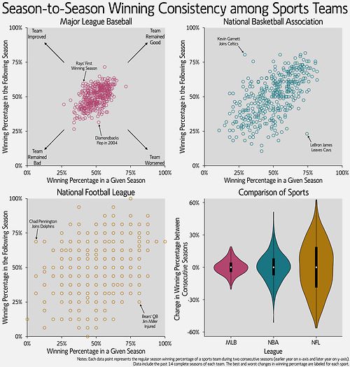
Take Major League Baseball for example. The MLB has an unreasonably wide range of payrolls.
In 2013, two teams had payrolls north of $216 million, with two additional teams having payrolls
north of $150 million. At the other end of the range, fully 16 teams (more than half the league)
had payrolls less than $100 million.

And unlike the NFL, it’s also easy to see a relatively strong connection between market size and
payroll. By a substantial margin, New York and Los Angeles are the most populous metropolitan
areas in the US; to wit, the Yankees and Angels had 2013 payrolls of $229,000,000 and
$216,000,000 respectively. Now the question is how does the disparity in terms of payroll
between teams translate into the competitiveness of the product on the field? It would stand to
reason that given additional financial resources a team would be able to acquire better players,
which would ultimately translate into more wins (unless of course you’re the 2013 Los Angeles
Angels). Thus, it stands to reason that a relatively tighter dispersion of payrolls across a sport
should lead to greater competitive balance.

However, the idea that the tighter dispersion of payrolls is what is responsible for the NFL’s
competitive balance ignores, or least obfuscates, a key point. That is, is the NFL season actually
long enough for any team’s win-loss record to be statistically significant? Putting it another way,
is the NFL season long enough for “true talent” to prevail?

If the NFL season and its playoff structure are such that we can’t glean any meaningful statistical
conclusions from it, then the idea that payroll parity promotes competitive balance is really
unfounded and the inter-season mean reversion we observe is more a result of the random
outcomes that can occur with too small a sample size and not from any characteristic of how the
league operates.

In a recent post on the MIT Sloan Sports Analytics Conference website, “Exploring Consistency
in Professional Sports: How the NFL’s Parity is Somewhat of a Hoax,” Brown University
Doctoral Candidate Michael Lopez dissected several measures of parity in sports. As the title
suggests, NFL parity is largely a mirage.
After several technical data transforms which make comparisons between sports more consistent,
Lopez gets to the heart of the matter: the NFL suffers from a small sample size. The NFL
regular season has only 16 games, whereas basketball and hockey have 82 and baseball has an
incredible 162. Because of the lesser number of games, it is more likely in the NFL that the
regular season record will not reflect the “true talent” of the team.

For example, Figure 2. shows a cumulative distribution function for win percentage of a
theoretical team in the NFL and MLB.

Figure 2. Comparison of Potential Win Percentages Between Theoretically Average NFL and
MLB Team

The chart shows the possible outcomes for a team given a 50% true talent (in other words, a team
whose ability would suggest they should win half of their games). The standard deviations of
team wins are gleaned from historical data and are 1.56 games for football and 10 games for
baseball. Even with the larger standard deviation in baseball (6.4x larger), the even
larger sample size in baseball (10.1x larger) imposes a central tendency to the possible
outcomes. In plain English, the number of games played in baseball makes us significantly more
confident that teams with the highest level of true talent will ultimately succeed in a given
season.

With 90% fewer games, football is unable to make such guarantees. In fact, looking at the teams
that actually made the playoffs since 2002, a perfectly average team will win enough games to
make the playoffs almost 20% of the time. While this may not seem so out of the ordinary,
remember that an average team has no business being in the playoffs at all.

But such is the way of the world when you suffer from small sample sizes; the error term
dominates the outcomes and weird things happen more often than your intuition would lead you
to believe.

The world of investing has a clear analog, though the situation is more complex. Consider two
investment teams where one team – Alpha Manager – has genuine skill while the other team –
Beta Manager – is a closet indexer with no skill. After fees Alpha Manager expects to deliver a
mean return of 10% per year with 16% volatility, while Beta Manager expects to deliver 8% with
18% volatility. Both managers are diversified equity managers, so the correlation of monthly
returns is 0.95.

With some simple math, and assuming a risk free rate of 1.5%, we can determine that Alpha
Manager expects to deliver about 3% in traditional alpha relative to Beta Manager. This is the
investment measure of ‘raw talent’.

Beta of Alpha Manager with Beta Manager (closet indexer) = (0.95 x 16% x 18%)/(18^2)=0.84
CAPM expected return of Alpha (skilled) manager = 1.5% + 0.84 * (8% – 1.5%) = 7%
Expected Alpha for Alpha Manager = 10% – 7% = 3%

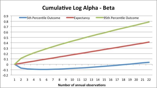
The question is, how long would we need to observe the performance of these managers in order
to confidently identify Alpha Manager’s skill relative to Beta Manager? Without going too far
down the rabbit hole with complicated statistics, Figure 3. charts the probability that Alpha
Manager will have delivered higher compound performance than Beta Manager at time horizons
from 1 year through 50 years. [If you want the worksheet, email us and I may consider sending it
out.]

Figure 3.

You can see from the chart that there is a 61% chance that Alpha Manager will outperform Beta
Manager in year 1 of our observation period. Over any random 5 year period Beta Manager will
outperform Alpha Manager about a quarter of the time, and over 10 years Beta will outperform
Alpha almost 15% of the time. Only after 20 years can we finally reject the probability that
Alpha Manager has no skill at the traditional level of statistical significance (5%). [Note this
version corrects a slight miscalculation in the original draft].

Figure 4. demonstrates the same concept but in a different way. The red line represents the
expected cumulative log returns to Alpha Manager relative to Beta Manager; note how it shows a
nice steady accumulation of alpha as Alpha Manager outperforms Beta Manager each and every
year. But this line is a unicorn. In reality, 90% of the time (assuming a normal distribution,
which is naive) Alpha’s performance relative to Beta will fall between the green line at the high
end (if Alpha Manager gets really lucky AND Beta Manager is very unlucky) and the blue line at
the low end (if Alpha Manager is really unlucky AND Beta Manger is really lucky). Note how in
5% of possible scenarios Alpha Manager is still under performing Beta Manager after 17 years
of observation!

Figure 4. 90% range of log cumulative relative returns between Manager A and Manager B at
various horizons

These results should blow your mind. They should also prompt a material overhaul of your
manager selection process. And it gets worse. That’s because the results above make very
simplistic assumptions about the distribution of annual returns. Specifically, they assume that
returns are independent and identically distributed which, as we’ve mentioned in previous posts,
they decidedly are not. In addition, certain equity factors go in and out of style, persisting very
strongly for 5 to 7 years and then vanishing for similarly long periods. Dividend stocks are this
cycle’s darlings, but previous cycles saw investors fall in love with emerging markets (mid-
naughts), large cap growth stocks (late 1990s), large cap ‘nifty fifty’ stocks (60s and 70s), etc.

Sometimes investment managers don’t fade with a whimper, but rather go out with a bang. Ken
Heebner’s CGM Focus Fund was the top performing fund of the decade in 2007, having
delivered 18% per year over the 10 years prior, a full 3% ahead of any other U.S. equity mutual
fund (source: WSJ). You might be tempted to believe that Ken is possessed of a supernatural
investment talent; after all, ten years is a fairly long horizon to deliver persistent alpha. And
indeed, investors did flock to Ken in droves. Unfortunately, as so often happens, most investors
jumped into his fund in 2007 – $2.6 billion of new assets were invested in CGM Focus in 2007
(source: WSJ).

Inevitably, Ken’s performance peaked in mid 2008 and proceeded to deal these investors a mind
melting 66% drop to its eventual month-end trough in early 2009. If you don’t have a calculator
handy, I’ll point out that at the fund’s 2009 trough it had wiped out over 12% in annualized
returns over the now almost 11 year period, bringing its annual return down under 6%.

What’s an investor to do if she can’t make meaningful decisions on the basis of track records?
Well, that’s the trillion dollar question, isn’t it. Unfortunately the only information that is
meaningful to investment allocation decisions is the process that a manager follows in order
to harness one or more factors that have delivered persistent performance for many years.
The best factors have demonstrable efficacy back for many decades, and perhaps even centuries.
For example, the momentum factor was recently shown to have existed for 212 years in stocks,
and over 100 years for other asset classes. Now that’s something you can count on.

That’s why we spend so much time on process – because we know that in the end, that’s the only
thing that an investor can truly base her decision on.

For the same reason, we are never impressed solely by the stated performance of any backtest –
even our own. Rather, we are much more impressed by the ability of a model to stand up under
intense statistical scrutiny: many variations of investment universes tested in multiple currencies
under several regimes, along with a wide range of strong parameters with few degrees of
freedom.

Often, we see firms advertising excellent medium-term results built on flimsy statistical grounds.
Without understanding their process in great detail, these results are meaningless. Less
commonly, we see impressive shorter-term sims, but that are clearly based on robust,
statistically-significant long-term foundations. In those cases, we sit up and take note because
statistically-significant, stable, long-term results are much rarer and much more important than
most investors imagine.

NFL parity – and far too often, investment results – are both mirages. Small sample sizes in any
given NFL season and high levels of covariance between many investment strategies make it
almost impossible to distinguish talent from luck over most investors’ investment
horizons. Marginal teams creep into the playoffs and go on crazy runs, and average investment
managers have extended periods of above-average performances.

The next time you observe a team or a manager on what appears to be a streak, it’s important to
remember that looks can be deceiving.

If you don’t believe us, just wait until next season.