No. 1112 2020 - Banco de la República
←
→
Page content transcription
If your browser does not render page correctly, please read the page content below
A Comprehensive History of
                                                                                                   Regression Discontinuity Designs:
                                                                                                   An Empirical Survey of the last 60
                                                                                                   Years

                                                                                                   By: Mauricio Villamizar-Villegas
                                                                                                       Freddy A. Pinzón-Puerto
                                                                                                       María Alejandra Ruiz-Sánchez

                                                                                                                                No. 1112
                                                                                                                                    2020

Bogotá - Colombia - B ogotá   - Bogotá - Colombia - Bogotá - Colombia - Bogotá - Colombia - Bogotá - Colombia - Bogotá - Colombia - Bogotá - Colombia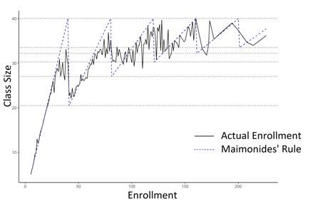
A Comprehensive History of Regression Discontinuity Designs:
                    An Empirical Survey of the last 60 Years∗

           Mauricio Villamizar-Villegas†                 Freddy A. Pinzón-Puerto‡
                               María Alejandra Ruiz-Sánchez§

The opinions contained in this document are the sole responsibility of the authors and do not
                    commit Banco de la República nor its Board of Directors

                                              Abstract

      In this paper we detail the entire Regression Discontinuity Design (RDD) history,
      including its origins in the 1960’s, and its two main waves of formalization in the
      1970’s and 2000’s, both of which are rarely acknowledged in the literature. Also, we
      dissect the empirical work into fuzzy and sharp designs and provide some intuition
      as to why some rule-based criteria produce imperfect compliance. Finally, we break
      the literature down by economic field, highlighting the main outcomes, treatments,
      and running variables employed. Overall, we see some topics in economics gaining
      importance through time, like the cases of: health, finance, crime, environment, and
      political economy. In particular, we highlight applications in finance as the most novel.
      Nonetheless, we recognize that the field of education stands out as the uncontested
      RDD champion through time, with the greatest number of empirical applications.

      JEL Classification: B23, C14, C21, C31, C52

      Keywords: Regression Discontinuity Design; Fuzzy and Sharp Designs; Empirical
      Survey; RDD Formalization

  ∗
    We thank the very useful research assistance provided by Tatiana Mora-Arbelaez and Juan David Yepes.
We also thank the valuable feedback from Rodrigo Villamizar.
  †
    Banco de la República, e-mail: mvillavi@banrep.gov.co
  ‡
    Universidad del Rosario, e-mail: freddy.pinzon@urosario.edu.co
  §
    Banco de la República, e-mail: mruizs@javeriana.edu.co
La Historia Sobre el Diseño de Regresión Discontinua
en los Últimos 60 Años
Mauricio Villamizar-Villegas Freddy A. Pinzón-Puerto
María Alejandra Ruiz-Sánchez
Las opiniones contenidas en el presente documento son responsabilidad exclusiva de los
autores y no comprometen al Banco de la República ni a su Junta Directiva
Resumen
En este artı́culo detallamos toda la historia sobre el Diseño de Regresiones Discontinuas
(RDD), incluyendo sus orı́genes en los 60s, y sus dos olas principales de formalización en los
años 70s y 00s, las cuales rara vez son reconocidas en la literatura. Además, diferenciamos el
trabajo empı́rico en diseños difusos y nı́tidos, y proporcionamos cierta intuición de por qué
algunos criterios basados en reglas producen asignación imperfecta. Finalmente, desglosamos
la literatura por campo económico, destacando los principales resultados, tratamientos y
variables de asignación empleadas. En general, vemos algunos temas en economı́a que cobran
importancia a través del tiempo, como los casos de: salud, finanzas, crimen, medio ambiente
y polı́tica económica. En particular, destacamos las aplicaciones en finanzas como las más
novedosas. No obstante, reconocemos que el campo de la educación se destaca como el
campeón indiscutible de RDD a través del tiempo, con el mayor número de aplicaciones
empı́ricas.
Clasificación JEL: B23, C14, C21, C31, C52
Palabras Clave: Regresión Discontinua; Diseño Nitido y Borroso; Formalización de
RDD“...a discontinuity, like a vacuum, is abhorred by nature” (Hotelling), yet “fluidity and discontinuity
are central to the reality in which we live in” (Bateson)1
1 Introduction
In this paper we bring together the entire Regression Discontinuity Design (RDD) literature;
namely 60 years in the making, and covering over 200 empirical papers. Our contribution is
threefold. First, we detail a comprehensive RDD history, including its origins (in the 60’s)
and its two main waves of formalization (in the 70’s and 00’s), both of which are rarely
acknowledged in the literature. Second, we dissect the literature into fuzzy and sharp designs
and provide some intuition as to why some rule-based criteria produce imperfect compliance,
i.e. cases in which treated and control observations are only partially enacted. Finally, we
break the literature down by economic field, highlighting the main outcomes, treatments, and
running variables employed.
In contrast to practical user guides such as Imbens and Lemieux (2008); Cook and
Wong (2008); Lee and Lemieux (2010); and DiNardo and Lee (2011), we do not provide a
step-by-step handbook of implementation procedures. Rather, we provide a comprehensive
outlook of the vast variety of existing designs within each field. Thus, RDD practitioners
can quickly extract and focus on the strand of literature closest to their investigation and be
warned about potential perils and pitfalls. We also provide a general theoretical framework
to familiarize readers with RDDs viewed as ex-post facto experiments. We finally reference
influential studies on some of the most technical issues.
The RDD history begins in the year 1960s, when Thistlethwaite and Campbell (1960)
used a discontinuity approach to measure the effect of students winning certificates of merit
when applying to college. A few years later, Sween et al. (1965)’s contribution to interrupted
time series paved the way to separately characterizing sharp and fuzzy designs. Surprisingly,
the methodology lay practically dormant for almost 40 years, except for the period that
we denote as the first wave in the 1970s, led by Goldberger (1972), Barnow (1972), Rubin
(1974), and Trochim and Spiegelman (1980), among others. This period is largely portrayed
by the pairings between Randomized Controlled Trials (RCTs) and approximations to true
experiments (quasi-experiments). When both are run in tandem, estimators can be combined
1
Harold Hotelling in “The Collected Economics Articles of Harold Hotelling” (pg. 52). Mary C. Bateson
in “Composing a Life” (pg. 13).
3and compared in terms of precision (efficiency) and unbiasedness. At this point in time,
however, RDDs were either viewed as a special case of Difference-in-Differences (Sween et al.,
1965), Matching (Heckman et al., 1999), or Instrumental Variables (Angrist and Krueger,
2001).
At the turn of the new millennium, we document the revival of RDDs with its second
wave of formalization, led by authors such as Hahn et al. (2001), Porter (2003), and Leuven
and Oosterbeek (2004). In particular, we acknowledge the pioneer works of Hahn et al. (1999)
and Angrist and Lavy (1999) in formally conducting sharp and fuzzy RDDs, respectively, in
the way that they are applied today.
Overall, there are several attractive features that embody RDDs, including the seemingly
mild assumptions needed for identification. Further, a well executed RDD produces similar
estimates to those from RCTs. This has led authors like Lee and Lemieux (2010) to state that
RDDs are “a much closer cousin of randomized experiments than other competing methods.”
Barnow (1972), Trochim and Spiegelman (1980), and Cook and Wong (2008) empirically
corroborate this by contrasting cases in which RDDs and purely experimental designs are
conducted (with overlapping samples) and show that, based on different criteria, they yield
similar results.
On the downside, it is not often the case that policy treatments are deterministically
triggered, so finding a suitable real-life case study is challenging. Also, a subset of problems
that apply to standard linear estimations carry over to RDDs (e.g. misconstruing non-
linearities for discontinuities). We also recognize that RDDs are subject to greater sampling
variance, and thus have less statistical power than a randomized experiment with equal sample
size, sometimes by up to a factor of three (Goldberger, 1972). Finally, being a localized
approach, if the design narrows in too close to the threshold, less observations become
available. This is why RDD is ultimately an extrapolation-based approach. Notwithstanding,
we show that the economic literature is growing ever more receptive to studies employing
RDDs.
In the entire literature, we see some topics in economics gaining importance through time,
like the cases of: health, finance, crime, environment, and political economy. In particular,
we highlight applications in finance as the most novel which, to the extent of our knowledge,
no other survey covers. In this area, most of the research has centered on the effects of
credit default on variables such as corporate investment, employment, and innovation. In
low-income countries, RDDs have been used to study the impact of microcredit programs on
4output, labor supply, schooling, and even reproductive behavior. We also document the use
of RDDs in procurement auctions, where neighboring bids reveal a similar valuation of the
underlying asset, and thus bidders are very similar except in actually winning the auction.
Nonetheless, we recognize that the field of education stands out as the uncontested RDD
champion through time, with a total number of 56 empirical studies. Arguably, the area of
labor is the runner up, with a total of 36 studies.
Our RDD inventory was compiled through a web-scrapping search across different
sources including RePEc, Scopus, Mendeley, and Google Scholar. We searched for studies
containing Regression + Discontinuity + Design (plural and singular) either in the title or
abstract. To avoid leaving some papers out of our analysis, we also conducted robustness
searches, for example studies with JEL classification categories pertaining to the letter “C”.
After manually revising each search result, and keeping only the most updated or published
version of each paper, we gathered a total of 205 studies, all of which are presented in our
Online Appendix. It reports each paper’s corresponding field, outcome variable, treatment,
running variable, cutoff value (and unit of measure), whether it employs a fuzzy or sharp
design, and key findings. Finally, for each paper we obtained the number of citations and
Web of Science -ISI impact factor (if published). Those with highest scores (most influential)
are largely analyzed in Sections 3 and 4.
We believe that RDD practitioners of all fields can benefit from our survey. For one, it
complements existing surveys and user guides such as Lee and Lemieux (2010), by including
at least a decade’s worth of new findings. Hence, while Lee and Lemieux cover a little over 60
studies up until 2009, we cover over 200 studies up until 2019, a significant nearly three-fold
increase in sample size. Also, we build on some of the extensions proposed by Lee and Lemieux.
In particular, the authors state that “there are other departures that could be practically
relevant but not as well understood. For example, even if there is perfect compliance of the
discontinuous rule, it may be that the researcher does not directly observe the assignment
variable, but instead possesses a slightly noisy measure of the variable. Understanding the
effects of this kind of measurement error could further expand the applicability of RD.” We
make emphasis on this point and more generally on cases where treatment is partially enacted
at the threshold. We also provide numerous examples of these fuzzy designs in Section 4,
that range from financial options not being exercised, to eligible beneficiaries of government
programs who are unwilling to take part.
52 Theoretical underpinnings of RDDs
This section sets the stage for the basic understanding of Regression Discontinuity Designs
(RDDs). While it intends to familiarize readers with its general framework, it does not
provide a thorough examination of some of its more technical aspects. In those cases,
however, we do direct readers to the most recent studies that have contributed to its overall
formalization. For ease in readability, we provide the following glossary of terms:
Ex-post facto experiment: A quasi-experiment where individuals (or measurable units) are not randomly assigned. With
the aid of tools and techniques, treatment and control groups can be comparable at baseline.
Running variable: Variable used to sort and deliver treatment (also referred to as the assignment variable).
Sharp designs: Designs where the rule-based mechanism perfectly (and deterministically) assigns treatment.
Fuzzy designs: Similar to sharp designs but allowing for noncompliers (e.g. control and treatment crossovers).
Potential outcomes: Hypothetical outcomes, e.g. what would happen if an individual receives treatment, regardless
if she actually received treatment.
Endogeneity: Mostly refers to missing information (self-selection or omitted variables) that is useful in
explaining the true effect of treatment (other endogeneity problems include simultaneity
and measurement error).
Kernel regressions: Non-parametric technique used to estimates non-linear associations. Kernels (and bandwidths)
give higher weight (or restrict) observations that fall close to the mean.
Parametric estimation: Estimations that assume probability distributions for the data.
Overlap assumption: Assumption that guarantees that similar individuals are both treated and untreated.
Local projections: Approximations conducted locally for each forecast horizon of interest.
2.1 RDD Viewed as an Ex-Post Facto Experiment
Essentially, RDDs are characterized by a deterministic rule that assigns treatment in a
discontinuous fashion. For example, in Thistlethwaite and Campbell (1960), students are
awarded a certificate of merit based on the CEEB Scholarship Qualifying Test. Exposure to
treatment (i.e. receiving the certificate of merit) is determined by scoring above a given grade,
creating a discontinuity of treatment right at the cutting score. Hence, the main underlying
idea of the design is for students scoring just below the threshold (control group) to serve as
valid counterfactuals to students who barely crossed the threshold (treatment group), had
they not received the award.
More formally, in the standard Sharp RDD setup, the assignment of treatment, Di , is
completely determined by a cutoff-rule based on an observable (and continuous) running
variable, Xi , as follows:
Di = 1 {Xi ≥ x0 } (1)
where 1 denotes an indicator function and x0 is the threshold below which treatment is
denied. The discontinuity arises because no matter how close Xi gets to the cutoff value
6from above or below (as in the case of test scores), the treatment, or lack of treatment, is
unchanged. Intuitively, the rule creates a natural experiment when in close vicinity of x0 .
If treatment has an effect, then it should be measured by comparing the conditional mean
of an outcome variable (or vector of outcome variables) at the limit on either side of the
discontinuity point:
Average Treatment Effect = E (Y1i − Y0i | Xi = x0 )
= E (Y1i | Xi = x0 ) − E (Y0i | Xi = x0 )
= lim E (Yi | Xi = x0 + ) − lim E (Yi | Xi = x0 + ) (2)
↓0 ↑0
where, for each individual i, there exists a pair of potential outcomes: Y1i if exposed to
treatment, and Y0i if not exposed. The final equality holds as long as the conditional distribu-
tions of potential outcomes, Pr (Y1i ≤ y | Xi = x) and Pr (Y0i ≤ y | Xi = x), are continuous
at Xi = x0 . Namely, this requires individuals to be incapable of precisely controlling the
running variable. To further illustrate, McCrary provides an example in which workers are
eligible for a training program as long as their income in a given period is at or below a
hypothetical value of $14. He shows that manipulation of the running variable yields too few
(and likely different) workers above the threshold, and too many workers just below.
To better conceptualize the RDD methodology as an ex-post facto experiment, consider
an example found in Kuersteiner et al. (2016a), who initially propose the following linear
regression model:
yi = α + βDi + γi , (3)
In the context of merit-based awards such as the one described in Thistlethwaite and Campbell
(1960), it is evident that the Ordinary Least Squares (OLS) estimator β does not precisely
capture the effect of treatment. That is, students with very good test scores (far from
the cutoff) are likely to also embody characteristics of high effort and ability. Thus, when
evaluating the effect of the scholarship award on future income, these other characteristics
would mask the true effect of treatment, leading to an upward bias. More formally, the bias
can be computed as the conditional mean of the error term with and without treatment,
E [γi |Di = 1] − E [γi |Di = 0], which would most likely be positive in this context.
In contrast, consider the same linear model but under a localized analysis around the
cutoff score. Any endogenous relationship is now broken down by the fact that small variations
in the running variable (Xi ), which lead to small variations in γi , generate a discontinuous
7jump in Di . It is precisely this variation that an RDD exploits in order to conduct causal
inference. Formally,
lim E [yi |Xi = x0 + ] − lim E [yi |Xi = x0 + ]
↓0 ↑0
= α + β + lim E [γi |Xi = x0 + ] − α + lim E [γi |Xi = x0 + ] = β. (4)
↓0 ↑0
As noted in equation (2), the RDD approach relies on the somewhat weak assumption that
unobservable factors vary smoothly around the cutoff. This is also exemplified in equation
(4) where the two conditional means of the error term (with and without treatment) cancel
out at the limit, when Xi = x0 . Further reading on this continuity assumption is presented
in Hahn et al. (2001), Porter (2003), Imbens and Lemieux (2008), and Lee (2008a). It allows
for the treatment (e.g. certificate of merit) to become uncoupled from unobservable factors
when narrowing locally at the threshold.
Imbens and Lemieux (2008) point out that local regressions improve over simple
comparison of means around the discontinuity point as well as over standard kernel regressions.
In turn, Kuersteiner et al. (2016b) provide a useful representation of RDDs applied to a
time series setting and with the use of local projections, as in Jordá (2005). The resulting
representation, based on Hahn et al. (2001), but with a cutoff-rule adapted to a time series
setting, where Dt = 1 {Xt ≥ x0 }, is presented as follows:
−J
J TX
X 2 Xt − x0
â, b̂, γ̂, θ̂ = arg min (yt+j − aj − bj (Xt − x0 ) − θj Dt − γj (Xt − x0 ) Dt ) K
a,b,γ,θ h
j=1 t=2
(5)
0
where θ = (θ1 , ..., θJ ) are the impulse-response coefficients that capture the impact of
treatment on outcome variables “j” periods after treatment, the term K (·) represents a
kernel function (where h is its bandwidth parameter), and bj , and γj are polynomial functions
of the running variable. The inclusion of the term γj (·)Dt allows for different specifications
of how the running variable affects the outcome, at either side of the cutoff.
We note that using a rectangular kernel with a sufficiently large bandwidth (using
information far from the discontinuity point) yields a global parametric regression, no different
from using OLS over the entire sample. More generally, the vector θ can be interpreted
as a weighted average treatment effect; weights being the relative ex-ante probability of
the running variable falling within the immediate neighborhood of the threshold (Lee and
Lemieux, 2010).
8An attractive feature of RDDs is that, by design, the Conditional Independence As-
sumption (CIA) is satisfied. For readers unfamiliar with this assumption, the CIA states that
conditional on an informative history, policies are independent of potential outcomes, or as
good as randomly assigned. This allows for the foundation based on which “regressions can
also be used to approximate experiments in the absence of random assignment”.2 Specifically,
the CIA can be formulated as:
Ykt ⊥ Dt | Xt for k = 0, 1. (6)
In the context of RDDs, the running variable carries all the information needed to construct
the policy variable, so the term Dt | Xt is purged from all information (recall that Dt is a
deterministic function of Xt ). This is the reason why the CIA is trivially met. As pointed
out by Lee and Card (2008), “One need not assume that RD isolates treatment variation that
is as good as randomly assigned, instead randomized variation is a consequence of agents’
inability to precisely control the assignment variable near the known cutoff.” The drawback,
however, lies in the impossibility of observing both treated and control observations for a
given value of xt , something that in the literature is referred to as the overlap assumption.
Hence, in any RDD approach, the continuity assumption of potential outcomes plays an
essential role. And, even though this assumption cannot be purely tested, it does have some
testable implications which are discussed in the following subsection.
We next turn our attention to cases in which treatment is partially enacted at the
threshold. In other words, where there is imperfect compliance. Examples of these fuzzy
designs range from financial options not being exercised, to eligible beneficiaries of government
programs who are unwilling to take part. In Section 4 we detail various examples covered in
the literature. In these cases, a valid design is still possible as long as there is a discontinuous
jump in the probability of being treated, even though the running variable does not perfectly
predict the treatment status. This necessary condition is exemplified as follows:
lim P r (Di = 1 | Xi = x0 + ) 6= lim P r (Di = 1 | Xi = x0 + ) . (7)
↓0 ↑0
For the most part, studies that conduct a fuzzy design carry out an instrumental variable
approach, by instrumenting the observed treatment status (i.e. whether an individual was
actually treated or not) with both the running variable and the treatment dictated by the
cutoff rule. As documented in Lee and Lemieux (2010), the treatment effect can then be
2
Angrist and Pischke (2009), pg 18.
9computed as the ratio between the jump in the outcome variable and the share of compliant
observations (those that are triggered by the rule and receive treatment), as follows:
lim↓0 E [Yi |Xi = x0 + ] − lim↑0 E [Yi |Xi = x0 + ]
. (8)
lim↓0 E [Di |Xi = x0 + ] − lim↑0 E [Di |Xi = x0 + ]
We note that this setting is also ideal for a broader type of designs, such as the case of a
continuous endogenous regressor.
2.2 Specification Testing: Perils and Pitfalls
Compared to other non-experimental approaches, RDDs require seemingly mild assumptions.
In particular, in order to have a locally randomized experiment, market participants cannot
perfectly control the running variable near the cutoff (Lee 2008). In principle, this assumption
is fundamentally untestable given that we observe only one realization of X for a given
individual (Xi ) or time period (Xt ). Nonetheless, McCrary (2008) proposes a test that has
become standard in the RDD literature: to analyze the bunching of observations in close
proximity of the threshold. In other words, the test estimates the density function of the
running variable at either side of the cutoff. Rejecting the null hence constitutes as evidence
of precise sorting (i.e. manipulation) or self-selection around the cutoff, a clear warning signal
that can ultimately compromises the validity of the design. However, some promising work
has been conducted when in the presence of heap-induced bias. For example, Barreca et
al. (2016) propose a “donut-RD” approach that estimates treatment after systematically
dropping observations in close vicinity of the threshold.
In addition, the estimated effect must be attributed solely to the treatment being
considered. To avoid type-I errors (i.e. a false positive), Hahn et al. (2001) argue that all
other factors must be evolving smoothly with respect to the running variable. Put differently,
the distribution of baseline covariates should not change discontinuously at the threshold.
Thus, predetermined variables, which include lagged outcome variables, should not predict
treatment when conditioning on the running variable. Studies that consider the possibility of
other discontinuous jumps at the same cutoff include Imbens (2004), Lee et al. and Battistin
and Rettore (2008).
Furthermore, a key concern in RDD analysis has to do with non-linearities, often
misconstrued as discontinuities. In this sense, a researcher generally decides over implementing
a parametric or non-parametric approach when estimating the effects of treatment. As stated
in Lee and Lemieux (2010) “If the underlying conditional expectation is not linear, the
10linear specification will provide a close approximation over a limited range of values of X
(small bandwidth), but an increasingly bad approximation over a larger range of values of X
(larger bandwidth)”. Note that if the methodology narrows in too close to the threshold, less
observations become available. This is why RDD is fundamentally an extrapolation-based
approach. A useful discussion on the choice of estimator is found in Hahn et al. (2001),
Porter (2003), and Imbens and Lemieux (2008). Everything considered, parametric and
non-parametric estimations should be seen as complementary and ideally report similar
findings.
Fortunately, a very recent (and growing) strand of literature has centered on the choice
of bandwidth. Given that a “correct” bandwidth parameter can only be unveiled when
knowing the true relationship between the outcome and running variables, several sensitivity
tests have been proposed. In particular, we refer readers to the works of Ludwig and Miller
(2007), Lee and Card (2008), Lemieux and Milligan (2008a), DiNardo and Lee (2011), Imbens
and Kalyanaraman (2012), Card et al. (2012), Calonico et al. (2014), and Arai and Ichimura
(2018), all of which base the criteria of a bandwidth choice on a corrected cross-validation
procedure.
2.3 RDD Extensions
Several extensions to the standard RDD setting have also been considered in the recent
literature. One example is the analysis of “placebo” jumps: discontinuities in outcome
variables when the running variable crosses other, non-relevant, thresholds (Imbens, 2004).
Another front being developed is the full extension of RDDs to time-series or panel settings.
This is particularly useful when the running variable carries some built inertia and, as a
consequence, control episodes get eventually mixed with treated observations as the time
horizon expands. Hence, the Stable Unit Treatment Value Assumption –SUTVA– described
in Rubin (1974) does not hold. Also, agents can incorporate the possibility of treatment
even before the rule is actually triggered. We refer readers to the work of Kuersteiner et al.
(2016b) for a technical application of these issues in the context of exchange rate options in a
time-series setting, or to Perez-Reyna and Villamizar-Villegas (2019) in the context of foreign
bond holdings in a panel setting.
Additionally, a growing strand of literature has focused on discontinuities found in
geographical borders. A pioneer study in this area is Card and Krueger (1994) who compare
food establishments in the border between two US states: New Jersey (treatment) and
11Pennsylvania (control), to examine the effect of raising the minimum wage on employment.
More recent studies include Dell (2010) who studies the effects of forced mining labor in Peru
and Bolivia, and Spenkuch and Toniatti (2018) who study regulations on political advertising
across different counties. In essence, the main challenges of geographical designs, as stated
in Keele and Titiunik (2015), include the possibility of: (i) spatial correlation, (ii) multiple
discontinuities at boundaries, and (iii) multiple identification assumptions for the different
measures of distance from the boundary. The reason why these challenges arise is due to
the fact that geographical borders are seldom set randomly. To correct for these, Keele and
Titiunik show that spatial RDDs are equivalent to standard RDDs with the inclusion of two
running variables: latitude and longitude coordinates.
Some authors place emphasis on the inclusion of covariates in order to increase accuracy
in RDD estimates (Calonico et al., 2019). In principle, treatment is locally independent
from any potential confounding effect at the threshold, which renders the inclusion of
control variables unnecessary. However, the number of observations decreases rapidly as the
bandwidth shortens. To this effect, Frölich and Huber (2018) propose an a non-parametric
method to account for observed covariates and show that it can reduce the asymptotic
variance as well as control for discontinuities in the covariate distribution. Similarly, Black et
al. (2005) and Imbens and Lemieux (2008) affirm that covariates can mitigate small sample
biases in RDDs.
An application that has gained momentum in the recent RDD literature deals with
heterogeneous treatment effects, i.e. cases in which the cutoff varies for each unit in the
sample. To date, most studies normalize the running variable to produce a pooled RD
treatment effect. However, Cattaneo et al. (2016) point out that this common practice does
not fully exploit all the available information. Namely, the authors show that the pooled
parameter can be interpreted as “the weighted average across cutoffs of the local average
treatment effects for all units facing each particular cutoff value”. Hence, a multi-cutoff
estimate that captures treatment effects at every cutoff value will most likely differ from the
pooled estimate (except under specific assumptions).
Finally, promising RDD work has been conducted in cases where: the running variable
is discrete (Lee and Card, 2008), the discontinuity point is unobserved (Porter and Yu, 2015),
and multiple running variables are employed (Foote et al., 2015). Also, when using: quantile
treatment effects (Frölich and Melly, 2008), likelihood functions (Otsu et al., 2013), and
dynamic treatment effects (Cellini et al., 2008). We believe that future work on the robustness
12of fuzzy designs’ inference will soon largely develop (Feir et al., 2016).
3 A Fuzzy History Through Time
In the year 1960, Regression Discontinuity was first implemented to measure the effect of 5,126
students winning certificates of merit compared to 2,848 students who simply received letters
of recommendation when applying to college (Thistlethwaite and Campbell, 1960).
Surprisingly, the methodology lay practically dormant for almost 40 years, except for the
period that we denote as the first wave of RDD formalization in the 1970s, led by Goldberger
(1972), Barnow (1972), Rubin (1974), and Trochim and Spiegelman (1980), among others.
This period is largely characterized by the pairings between randomized controlled trials
and approximations to true experiments. When both are run in tandem, estimators can be
combined and compared in terms of precision (efficiency) and unbiasedness.
At the turn of the new millennium, we document the revival of RDDs with its second
formalization wave, led by authors such as Hahn et al. (1999), Angrist and Lavy (1999), Hahn
et al. (2001), Porter (2003), Leuven and Oosterbeek (2004), McCrary (2008), and Imbens
and Kalyanaraman (2012).
3.1 RDD Origins
Campbell and Stanley (1963) are probably pioneers in formalizing RDD procedures, by
examining the validity of experimental designs against common threats to causal inference.
However, Sween et al. (1965)’s contribution to interrupted time series allowed for a more
in-depth examination of RDDs and even paved the way for Campbell (1969) to separately
characterize sharp and fuzzy designs. That is, to differentiate between cases in which treatment
is fully (i.e. sharp) or partially (i.e. fuzzy) enacted at the threshold. More formally, Sween et
al. (1965) propose three tests to disentangle treatment from purely random variation:
1. Mood test: T-test significance of the first post-treatment observation from a value
predicted by a linear fit based on pre-treatment observations,
2. Walker-Lev tests: A set of tests to determine pre and post-existing differences
(regression slopes) between treated and control groups, and
3. Double Extrapolation technique: Significance test of the difference between two
separate regression estimates for a given outcome, for the observation midway between
13the last pre-treatmet point and the first post-treatment point.
While the Mood and Walker-Lev tests share similar features to event studies and difference-
in-difference methodologies, respectively, the double extrapolation technique narrows in on
the vicinity of treatment, and as such constitutes one of the first attempts to formally obtain
localized treatment effects.
Interestingly, Campbell explains why the national merit scholarships were unfit to use
a sharp design of actual college fellowships, as ideally depicted in Figure 1(a). According to
the author, pooling rankings of different groups of students across evaluating committees
“provides one cutting point on an unspecified pooled decision base, but fails to provide analogous
potential cutting points above and below ”, leading to a fuzzy design, exemplified by Figure
1(b), in which the CEEB Scholarship Qualifying Test does not perfectly predict treatment.
At the time, and without any formal fuzzy toolkits at hand, Campbell makes the following
recommendation: “If political patronage necessitates some decision inconsistent with a sharp
cutoff, record these cases under the heading ‘qualitative decision rule’ and keep them out
of your experimental analysis”.
(a) (b)
Figure 1: Computer-generated RDD data taken from Campbell (1969).
3.2 First Formalization Wave
During the 1970s, a handful of authors sought ways to implement RDDs applied to a variety
of scenarios. In most cases, they focused on bias reduction techniques based on the eligibility
criteria to receive treatment. This small group of RDD advocates, which favored discontinuity
designs as a preferred evaluation approach, are part of what we denote the first formalization
wave.
14We first document Barnow (1972), who evaluates education programs when group
selection is not random (or similarly, in the absence of pre-treatment information). Building
on some previous work by Campbell and Erlebacher (1970), Barnow presents four models
geared to demonstrate that biases can be avoided if randomization procedures or quasi-
experimental techniques are used, including RDDs.
Specifically, the first model considers the case where treatment and control groups are
selected from two different samples, with different sample means. In the model, x∗ is defined
as the true ability. The pre and posttest scores are given by xi = x∗i + ui and yi = x∗i + vi ,
respectively, both of which are erroneous measures of true ability. Namely, if a child gets a
score higher than her true pretest ability (xi ≥ x∗i ), then there is no prior knowledge about
whether she will get a score higher or lower than her true posttest ability. Hence, scores are
unbiased but do not reflect true ability. In the second model, gain scores (defined as yi − xi )
are regressed on the treatment dummy. While unbiased, estimates are invalidated under
heteroskedasticity or non-zero growth rates of ability over time. The third model includes
socioeconomic information so that group assignment is random within each socioeconomic
group. Finally, the fourth model considers a discontinuous regression model where children
are assigned treatment based on their pretest score. As stated in Barnow (1972), the latter is
the only valid case.
In a practical example, Goldberger (1972) analyzes compensatory educational programs
that had been criticized because students were not randomly selected (students with lower
capacity were selected in the treatment group and students with higher capacity in the control
group). Thus, even if the program had no effect on any outcome variable, at face value it
reported a negative impact. To illustrate this point more formally, consider the following
equation:
yi = β0 + β1 Di + β2 xi + ηi (9)
where Di is a dummy variable denoting whether the individual received treatment, and
the pre and posttest are again defined as erroneous measures of true skill: xi = x∗i + ui ,
yi = x∗i + vi . Under the assumption that treatment has a null effect, Goldberger assesses
two particular cases, namely when:
1. individuals are assigned treatment whenever their true skills lie below the true mean
skill, x∗i < x̄∗i
152. individuals are assigned treatment whenever their pretest scores lie below the pretest
mean, xi < x̄i
For ease in notation, variables are centered at zero so that x̄∗i = x̄i = 0. In the first case,
and given that we only observe xi , then the regression result attributes spurious effects to
treatment in the posttest. Put differently, β1 6= 0 denotes the resulting bias. The source of
this bias lies in the imperfect selection procedure that assigns a few low-skilled (high-skilled)
individuals to the control (treatment) group. As observed in Figure 2(a), differences in true
ability of these cases (those in the control group with negative pretest scores and those in
the treatment group with positive pretest scores) are carried over to differences in posttest
scores. As a result, the coefficient β1 , which is captured by the differences in group intercepts,
reports a negative bias.
In the second case, note that the control group can include low-capacity individuals
with unusually high scores in the pretest, and vice-versa. However, since Di is completely
determined by the pretest score, it does not contain additional information about x∗i (i.e. the
only explanatory power that Di has on yi is through xi ). As shown in Figure 2(b), the bias
is now eliminated and β1 = 0.
(a) (b)
Figure 2: Selection procedure (pre and posttest scores in x and y-axis); Goldberger (1972).
Finally, Goldberger finds that the bias-free RDD estimate (where treatment assignment
is based on the pretest score) produces the same unbiased estimate as the case of purely
random selection. However, an RDD is subject to greater sampling variance, which means
16that random selection provides a more efficient design. The magnitude of this efficiency loss
is reported as follows: a random sample of size 100 is as good as a selected pretest sample of
size 275. Hence, the controlled experiment is 2.75 times more efficient than RDDs, due to
the correlation between the assignment variable and the cutoff.
We next turn our attention to Trochim and Spiegelman (1980) who propose an analytical
solution known as the “relative assignment variable approach” for the problem of pretest-
posttest selection bias. In essence, the relative assignment variable is simply the estimated
probability of treatment, conditional on the pretest. It bears the same meaning today as
a propensity score, commonly used in matching techniques. More formally, if we consider
the specification in equation 9, then the validity of the treatment effect, β1 , will ultimately
depend on the estimand of E[Di |xi ].3
Trochim and Spiegelman establish three methods for estimating the probability of
treatment.4 The first is called “assignment percentage” where individuals are sorted by their
pretest values and divided into equal size intervals. Then, the percent of cases assigned to
the program is calculated for each interval, and those values are assigned to individuals. The
second method is called “nearest neighbor moving average” and essentially computes the
moving average of Di ’s for the close neighbors of xi , including xi .5 The last method uses a
maximum likelihood Probit model under which the probability of treatment is equal to the
estimated cumulative normal distribution, i.e. P r[Di = 1|xi ] = Φ(zi0 β̂).
To exemplify, Trochim and Spiegelman present four model designs with different
assignment strategies. The first is a randomize experiment, where E[Di |xi ] is constant for
any pretest value and can be described by a horizontal line relative to xi , as shown in Figure
3(a). While this case does not require a pretest, it is included in equation 9 to increase the
statistical power of the program effect estimate. The second model is a sharp design where
treatment is based on scoring above a cutoff-value. Hence, E[Di |xi ] = 0 for individuals with
a pretest value lower than the cutoff and E[Di |xi ] = 1 for those with a pretest value greater
or equal than the cutoff, as shown in Figure 3(b). Finally, the third and fourth models
are a fuzzy design and a non-equivalent group, where assignment is based on non-random
decision factors. For these two cases, E[Di |xi ] oscillates between the horizontal line of the
true experiment and the step function of the sharp design, as depicted in Figure 3(c).
3
Note that E[Di |xi ] = 1 · P r[Di = 1|xi ] + 0 · P r[Di = 0|xi ].
4
These methods are originally proposed in Spiegelman (1976), Spiegelman (1977), Maddala and Lee (1976)
and Barnow et al. (1978).
5
The number of neighbors vary depending on the width of the moving average window.
17(a) (b) (c)
Figure 3: Conditional probability of treatment; as in Trochim and Spiegelman (1980).
In most cases, the “relative assignment variable” successfully produces unbiased esti-
mates. However, it is unclear whether results hold under more realistic or complex scenarios,
for example when considering pretest-posttest nonlinear relationships or non-random assign-
ment close to extreme values of the pretest distribution.
3.3 Second Formalization Wave
At the turn of the millennium, Hahn et al. (1999) is one of the first studies that formally
conducts a sharp RDD, allowing for variable treatment effects. The authors evaluate the
effect of a federal anti-discrimination law on firm employment of minority workers, using
demographic data from the National Longitudinal Survey of Youth. Specifically, the authors
define the running variable as a the number of employees of a given firm, and consider
treatment as any firm with 15 employees or more, which was covered by the law. Within
their findings they show that, for at least two years, the Equal Employment Opportunity
Commission coverage had a positive effect on the percentage of minority workers employed
by small firms.
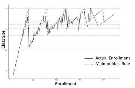
We document the work of Angrist and Lavy (1999) as one of the first formal applications
to fuzzy designs. The authors set their identification strategy around the Maimonides’ Rule
(named after the 12th-century rabbinic scholar Maimonides) to study the effects of class size
on students’ achievements in Israel. Formally, the rule is characterized as follows:
fsc = es /[int((es − 1)/40) + 1] (10)
where fsc denotes the number of students in classroom c of school s, es is the beginning-
of-the-year enrollment, and the function int(n) corresponds to the largest integer less than
or equal to n. Hence, enrollment cohorts of 41-80 are split into two classes of average size
1820.5-40, cohorts of 81-120 are split into three classes of average size 27-40, and so on. Figure
4(a) and 4(a) shows the actual class size compared to the Maimonides’ Rule for two years in
elementary school (4th and 5th grade, respectively), as used by Angrist and Lavy. As shown,
there was imperfect compliance to the rule, due to the many factors involved. For instance,
schools with a high Percent Disadvantage Index receive funds that are sometimes earmarked
for additional classrooms.
(a) (b)
Figure 4: Class size in 1991 by actual size and as predicted by Maimonides’ Rule in (a)
Fourth and (b) Fifth grade. Replication made using data from Angrist and Lavy (1999).
As such, Angrist and Lavy conduct an instrumental variable approach, common in the
recent RDD setup (see Section 2.1), with the following first and second stages:
0
First Stage: nsc = Xs π0 + fsc π1 + sc (11)
0
Second Stage: ȳsc = Xs β + nsc α + ηs + µc + usc (12)
where nsc denotes the actual classroom size, fsc is the class size as dictated by Maimonides’
0
Rule, and Xs is a vector of school-level covariates that include functions of enrollment,
student’s socioeconomic status, as well as variables identifying the ethnic character and
religious affiliation. In turn, ȳsc is the average class score, and ηs , µc capture within-school
and within-class correlation in scores. As a result, Angrist and Lavy find a negative effect of
class size on test scores for mathematics and reading scores. More specifically, they find that
smaller classes (i.e. classes with 10 fewer students) achieve a 75% higher grade score.
We finally document the work of Leuven and Oosterbeek (2004) who conduct both
sharp and fuzzy designs to evaluate the effects of tax deductions on training participation,
and the effects of training participation on wages, respectively, for the case of the Netherlands.
Essentially, the authors exploit a tax deduction, enacted in 1998, for firms that trained
19employees aged 40 years or more. This deduction translates into a cost discontinuity, with a
significantly lower cost of training someone right at the age of 40 years than someone right
below 40. Hence, to evaluate the effect of tax cuts on training participation, Leuven and
Oosterbeek estimate the following model:
E[ti ] = α + βdi (13)
where ti denotes the probability of receiving training and α is the probability of receiving
training without a tax deduction. The coefficient of interest, β, is interpreted as the change
in training probability due to the extra tax deduction in the vicinity of ā = 40 years of age,
i.e. lim↓0 E (t | a = ā + ) − lim↑0 E (t | a = ā + ).
Alternatively, the authors evaluate the effects of training participation on wages. Given
that the probability of training does not necessarily match the actual realization of being
trained, they estimate the following fuzzy design:
E(wi ) = ω + γ(ti ) (14)
where ω denotes the wage (in logs) without training, and ti is instrumented with the probability
of treatment as a function of age, P r(ti ) = f (ai , 1[ai ≥ ā]). The coefficient of interest, γ, is
interpreted as the localized change in wages due to training. Results in Leuven and Oosterbeek
(2004) show that employees just over 40 years of age have 15 - 20% higher probability of
training than those below 40 years. However, they find a null effect of participation on
wages.
4 RDDs by Economic field (in alphabetical order )
In this section we break the RDD literature down by economic field, highlighting the
main outcomes, treatments, and running variables employed. We also report the historical
distribution of fuzzy versus sharp designs and provide some intuition as to why some criteria
produce imperfect compliance (cases in which treated and control observations were partially
enacted). Most of our analysis in this section is based on literature from the new millennium,
since we note that only 12 empirical RDD studies were conducted before the year 2000
(mostly centered in issues pertaining to education and political economy).
As depicted in Figure 5, during 2004-2011, we observe over 76 studies, covering a wider
range of fields, including: education (25), labor market (16), health (11), political economy
20(9), finance (9), environment (3), and crime (3). Notably, the number of sharp designs during
this period nearly doubled the number of fuzzy designs (this is more clearly seen in Table 1).
The last time period dates from 2012 until 2019, and shows an even larger increase in the
number of empirical RDD applications, with close to 109 studies, most of which center on
education (22) and labor market (18).
Overall, we see some topics in economics gaining importance through time, like the
cases of: health, finance, crime, environment, and political economy. Nonetheless, education
stands out as the uncontested champion through time, with a total number of 56 empirical
studies out of a total of 205.
Overall, we see some topics in economics gaining importance through time, like the
cases of: health, finance, crime, environment, and political economy.
Figure 5: Empirical studies by economic field and type of design: 1996-2019.
21Table 1: Empirical studies by sharp or fuzzy design: 1996-2019
Sorted Alphabetically Fuzzy Sharp Both Total
Crime 5 4 0 9
Education 33 20 3 56
Environmental 5 9 0 14
Finance 12 14 0 26
Health 18 11 0 29
Labor market 13 19 4 36
Pol. Econ 4 21 3 28
Others 3 3 0 6
Total 93 101 10 204
4.1 Crime
In the area of crime, RDDs have been applied in research topics related to the evaluation of
prison’s risk-based classification systems, the effects of incarceration, prison conditions, and
the deterrence effect of criminal sanctions, among others. In this field we acknowledge the
pioneer and seminal paper by Berk and Rauma (1983), who examine unemployment benefits
to prisoners after their release. Also, in Table 2 we document popular treatments that range
from prison’s security levels and the severity of punishments, to educational levels. Outcome
variables generally focus on the number of arrests, inmates misconduct, post-release behavior,
and juvenile crime.
Table 2: Common variables in Crime
Relative frequency Common outcomes Common Treatment and Running variable Fuzzy/Sharp
20% Inmates misconduct and Arrest rates Prison security levels ←→ Classification score Fuzzy
20% Post-release criminal behavior Severity of punishments ←→ Age at arrest and adjudication score Fuzzy/Sharp
20% Juvenile crime Delayed school starting age ←→ Birthdate Fuzzy/Sharp
We find that roughly 56% of the crime literature employs fuzzy designs (see Table 1),
with date of birth and prisoners’ classification scores as commonly used running variables.
For instance, Berk and de Leeuw (1999) evaluate California’s inmate classification system,
where individual scores are used to allocate prisoners to different kinds of confinement
facilities. For example, “sex offenders are typically kept in higher-security facilities, because a
successful escape, even if very unlikely, would be a public relations disaster ” (pg. 1046). The
fuzziness in this case study stems from administrative placements decisions (different from
the score), based on practical exigencies, such as too few beds in some facilities or too many
in others.
22Also, Lee and McCrary (2005) evaluate the deterrence effect of criminal sanctions on
criminal behavior by comparing outcomes around the 18 year-age-of-arrest threshold. In
particular, the authors exploit the fact that offenders are legally treated as adults the day
they turn 18 and hence are subject to more severe punitive adult criminal courts. However,
all states in the US have the option to transfer a juvenile offender to a criminal court to be
treated as an adult (according to the authors, this is particularly the case in Florida). Thus,
the study corrects treatment assignment with a fuzzy framework.
4.1.1 Deterrence effects of incarceration
The crime literature generally establishes that increasing the severity of punishments deters
criminal behavior by raising the “expected price” of committing a crime. This approach is
supported by Becker (1968), who was one of the first authors to claim an inverse relationship
between criminal behavior and the likelihood of punishment. Henceforth, several authors have
been interested in providing empirical evidence indicating that court sanctions are effective
in reducing criminal behavior.
A more recent example is Hjalmarsson (2009), who analyzes the impact of incarceration
on the post-release criminal behavior of juveniles. The author exploits institutional features of
the justice system, namely discontinuities in punishment that arise in the state of Washington’s
juvenile sentencing guidelines. More specifically, these guidelines consist of a sentencing grid
that establishes punishment based on the severity of the offense and the criminal history
score. In this setting, an individual is sentenced to a state facility for a minimum of 15 weeks
if he/she falls above a cutoff, otherwise, the individual receives a minor sanction (i.e. fine or
probation). Results in Hjalmarsson indicate that incarcerated individuals are less prone to
be re-convicted of a crime.
Additionally, Lee and McCrary (2005) investigate the deterrence effect of jail-time on
criminal behavior. The underlying endogeneity problem is that, by design, severe criminal
sanctions receive lengthier times of incarceration. To overcome this problem, the authors
exploit the fact that when an individual is charged with a crime before his 18th birthday, his
case is handled by juvenile courts. In contrast, if the offense is committed during or after his
18th birthday, it is handled by the adult criminal court, affronting a more punitive criminal
sanction. Surprisingly, Lee and McCrary find that individuals are greatly unresponsive to
sharp changes in penalties. This result is consistent with extremely impatient or myopic
individuals, who essentially are unwilling to wait a short amount of time to see their crime
23sentence significantly reduced.
4.1.2 Prisoners’ placement
With a growing number of convict populations and ever tighter budget constraints, prison
systems have been looking for measures to improve their efficiency. And, a key criterion for
an effective placement is defined by the capability of controlling inmates’ misconduct. We
find several authors that provide an evaluation of how well the system currently allocates
inmates to incarceration facilities.
For instance, Berk and de Leeuw (1999) provide an evaluation of the inmate classification
system used by the State of California. Namely, the Department of Corrections estimates
a classification score that captures the likelihood of potential misconduct. This likelihood
includes a linear combination of controls, such as an inmate’s age, marital status, work history,
and above all, the length of the sentence, which accounts for almost 70% of the variance in
the overall classification score. After the score is computed, placement is undertaken. Berk
and de Leeuw conclude that the existing scores successfully sort inmates by different levels of
risk, and thus, assignment based on sorted security-level facilities reduce the probability of
misconduct.
Similarly, M. Keith and Jesse M. (2003) evaluate the effect of prison conditions on
recidivism rates, exploiting discontinuities in the assignment of prisoners to security levels
based on a score that reflects the need for supervision. The authors use a sample of 1,205
inmates released from federal prisons in the year 1987, with data on physical and social
conditions of confinement as well as post-release criminal activity. The authors find that
harsher prison conditions significantly increase post-release crime.
4.1.3 Crime and other economic fields
We finally document some studies that center on the causal relationship between crime and
other economic fields. Berk and Rauma (1983) for instance, evaluate ex-offenders’ eligibility
for unemployment benefits on reincarceration rates. That is, inmates in the state of California
are eligible for unemployment benefits if they enroll in vocational training programs or work
in prison jobs. The authors compare individuals with and without unemployment benefits
after their release and find that benefits effectively reduce recidivism.
In turn, Depew and Eren (2016) explore the link between school entry age (as previously
reported in Section 4.1) and crime. Specifically, the authors compare incidences of juvenile
24crime in the state of Louisiana, by neighboring in on the interaction between birth dates
and official school entry cutoff dates, and find that late school entry reduces the incidence of
juvenile crime for young black females, particularly in high crime areas. Somewhat related,
Cook and Kang (2016) investigate whether there is a causal link between student dropouts
and crime rates. The authors first demonstrate that children born just after the cutoff date
for enrolling in public kindergarten are more likely to drop out of high school. The authors
then present suggestive evidence that dropout precedes criminal involvement.
4.2 Education
While studies in the field of education cover an ample range of issues, most however relate
to student performance. As Table 3 shows, most studies (66%) center on either academic
achievement or educational attainment while others (21%) center on student enrollment or
access to higher education. Common treatment variables for the former include: summer
school attendance, class size, a delayed school starting age, and monetary incentives to
teachers. On the other hand, treatments for enrollment and access to higher education
include attendance and financial aid.
Table 3: Common variables in Education
Relative frequency Common outcomes Common Treatment and Running variable Fuzzy/Sharp
Summer school Attendance ←→ Test scores Fuzzy
Class Size ←→ Student enrollment Fuzzy
Delayed school starting age ←→ Birth date Fuzzy
66% Academic achievement or educational attainment
Attending better schools ←→ Admissions Exam score Fuzzy
Monetary incentives to teachers ←→ Program eligibility criteria Sharp
Attending better schools ←→ Admissions Exam score Fuzzy
21% Enrollment or access to higher education
Financial aid ←→ Program eligibility criteria Sharp
We observe that almost 59% of the entire education literature employs fuzzy designs (see
Table 1). This is particularly the case for studies that choose test scores as a running variable.
In Jacob and Lefgren (2004b) for instance, remedial programs were assigned to students
scoring below a passing grade. However, the authors note that some failing students received
waivers from summer school and some passing students were retained due to poor attendance.
In Jacob and Lefgren (2004a), the same authors evaluate the effects of teacher training in
schools that were placed on probation under the Chicago Public System. Among the several
estimation challenges, the authors note that: (i) student mobility (between probation and
non-probation schools), (ii) schools that were later placed on probation, and (iii) schools that
25You can also read