Non-proportional hazards - an introduction to their possible causes and interpretation - Jonathan Bartlett University of Bath thestatsgeek.com ...
←
→
Page content transcription
If your browser does not render page correctly, please read the page content below
Non-proportional hazards – an introduction to
   their possible causes and interpretation

               Jonathan Bartlett
               University of Bath
               thestatsgeek.com

                29th April 2021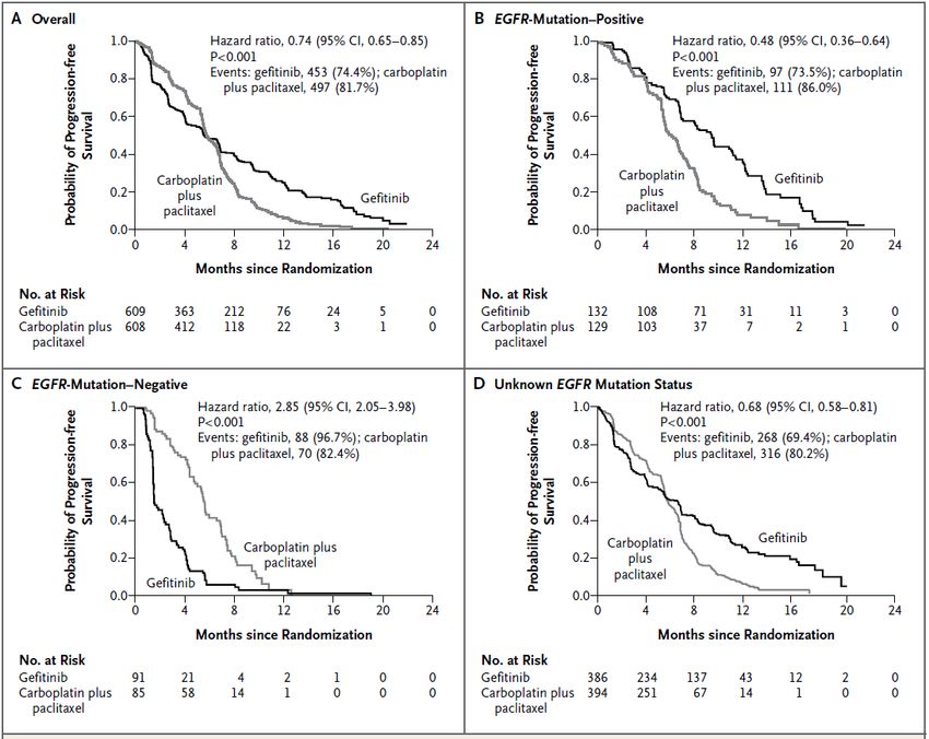
The Cox model and proportional hazards

Interpreting changes in hazard

Interpreting changes in treatment group HRs

HR under proportional hazards
The Cox model and proportional hazards
Basic randomised trial setup

   Randomised trial with control TRT = 0 and active TRT = 1
   patients.
   We measure time to event T .
   Some patients are censored: ∆ = 1 means event observed, ∆ = 0
   means event censored.
The hazard function

   The hazard function at time t, h(t) is the instantaneous rate of
   failure among survivors at time t:

                              P(t ≤ T < t + ∆t|T ≥ t)
                 h(t) = lim
                         ∆t→0           ∆t

   It is the failure rate at time t conditional on not yet failing (the
   T ≥ t bit).
The Cox model
Cox’s famous model, if we put only TRT as covariate, assumes that
h(t|TRT ) = h0 (t) exp(βTRT )
h0 (t) is an arbitrary baseline hazard function.
For any t, the hazard ratio (HR) comparing active to control is
h(t|TRT = 1) h0 (t) exp(β)
= = exp(β)
h(t|TRT = 0) h0 (t) exp(0)
which is independent of t.
Hazards between groups are proportional over time (PH).
If this is violated, we say hazards are not proportional (NPH).An example of NPH The PH assumption can be assessed in various ways. In recent years that have been various trials where NPH is indicated. E.g. the IPASS study (PFS Schoenfeld plot shown from Lin et al. (2020)):
Consequences of NPH

  The Cox model / log rank test has optimal power under PH. Under
  NPH, should we use a different test, and if so which?
  Under NPH how should we quantify the treatment effect? Should
  the effect estimation be strongly tied to the hypothesis test?
  What can cause NPH, and how should changes in the HR over time
  be interpreted?
Interpreting changes in hazard
Interpreting changes in hazard and HRs

   Interpreting changes over time in hazards and HRs is quite tricky,
   e.g. see Hernán (2010) ‘The Hazard of Hazard Ratios’.
   The source of the difficulty is due to the fact the hazard is a
   conditional (on survival) quantity and because of the ubiquitous
   presence of unmeasured/unknown patient level factors which
   influence outcome (frailty).
   I will demonstrate through a series of simple simulations, but see
   Chapter 6 of O. Aalen, Borgan, and Gjessing (2008) for further
   details.
A simple example

   Consider a single arm study.
   Suppose first that the hazard for time to event is a constant 1 for
   all patients, i.e. the hazard for each patient is h(t) = 1 for all t.
   So the hazard does not change with time in any patient.
   For simplicity, we will simply censor everyone who has not yet failed
   at t = 3
   We run our study, and look at the cumulative hazard to see if the
   hazard is constant over time
A simple example

                       3.0
   Cumulative hazard

                       2.0
                       1.0
                       0.0

                             0.0   0.5   1.0   1.5   2.0   2.5   3.0

                                                t

   The slope is constant at 1 → the hazard is constant.
Adding frailty (unmeasured prognostic covariates)
I In reality there will always exist factors which affect outcome
I Suppose there exists some gene (as yet unknown and hence
unmeasured) which affects time to event
I We will code the gene Z as a binary variable, with 50% Z = 0
and 50% Z = 1
I Then we assume
h(t|Z = 0) = 0.5
h(t|Z = 1) = 1.5
I For each patient, the hazard is 0.5 or 1.5, and doesn’t change
over time.
I We again run our study, and estimate the hazard function over
time in the whole groupCumulative hazard with frailty
2.0
Cumulative hazard
1.5
1.0
0.5
0.0
0.0 0.5 1.0 1.5 2.0 2.5 3.0
t
The slope (hazard) appears to decrease over timeInterpreting changes in hazard over time
I How do we interpret the apparent change in hazard over time?
I The most obvious that the hazard individuals experience
decreases over time.
I But we know we generated the data so that each individual’s
hazard is constant over time.
I What’s going on?Distribution of Z in risk sets
0.5
Proportion with $Z=1$ in risk set
0.4
0.3
0.2
0.1
0.0 0.5 1.0 1.5 2.0 2.5 3.0
TimeThe odd effects of frailty
I At t = 0, 50% of patients are Z = 0 and 50% are Z = 1
I The Z = 1 patients have higher hazard, so they fail more
quickly
I At times t > 0, among those still at risk, the mean/proportion
of patients with Z = 1 is less than 50%.
I So the group/population level hazard decreases, even though
the individual level hazards do not change over time.
I This is the effect of frailty - unobserved covariates which
influence hazard.
I Our plot is looking at the population or marginal (to Z ) hazard
function, not the individual hazard.Implications of frailty
I Interpreting changes in hazards, over time, is tricky.
I Changes can be a result of a combination of changes in
individual hazards over time and frailty/selection effects.
I With a single failure time per patient, from the data alone we
cannot really disentangle what is causing the observed changes
in population hazard.
I What implications does this have for hazard ratios comparing
treatment groups?Interpreting changes in treatment group HRs
Time specific HR for treatment
I Now we return to the arm trial setting.
I The true (i.e. without assuming any model)
population/marginal HR at t, HR(t), comparing active to
control is
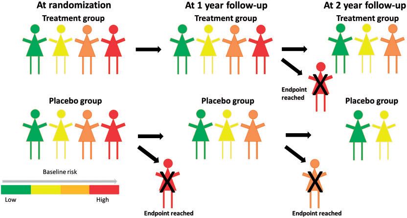
P(t≤TImbalance between treatment groups survivors in pictures. . . Taken from Stensrud et al. (2019).
Time-dependent HRs are generally subject to confounding

    I In general the answer is no due to frailty effects (i.e. Z )
    I The two groups of survivors at time t > 0 have different
      distributions of these baseline factors.
    I HR(t), and measures derived from it (e.g. piecewise HRs,
      weighted HRs) are generally not valid causal measures of
      treatment effect - they are subject to confounding.
    I These concerns have led to some researchers, particularly those
      from a causal inference background, rejecting use of HRs
      (especially time-dependent ones) as valid measures of
      treatment effect. (Hernán 2010; O. O. Aalen, Cook, and
      Røysland 2015; Martinussen, Vansteelandt, and Andersen 2018;
      Stensrud et al. 2019)
Interpreting changes in treatment group HRs
I We will consider two types of NPH: delayed effects and
diminishing effects
I We will simulate data so we know the truth
I We will compare this with what we can observe/estimate from
the dataIPASS Recall the IPASS Schoenfeld plot. The apparent interpretation is that initially chemo (control) is better for patients, but later Gefitinib is better. The estimated HR in the first 6 months is 1.115 and from 6 months onwards is 0.343 (Lin et al. 2020).
Simulated apparent delayed effect
   Results from some simulated data:

                                1.0

                                                                          1.0
                                                   Control
                                                   Active
                                0.8
         Survival probability

                                                                          0.5
                                                              log HR(t)
                                0.6

                                                                          0.0
                                0.4
                                0.2

                                                                          −1.0
                                0.0

                                      0.0   1.0   2.0   3.0                      0.0   1.0   2.0   3.0

                                                                                         Time

    I Benefit of active treatment appears to emerge later in f/up
    I In fact active even seems slightly worse than control initially
How the data were simulated
I The data were simulated with
h(t|Z , TRT ) = exp(Z − TRT + 2Z × TRT )
I True log HR for Z = 0 patients is -1, or HR of exp(−1) = 0.4.
I True log HR for Z = 1 patients is +1, or HR of exp(1) = 2.7.
I The individual level HRs for treatment effects do not vary over
time!
I The time changing population level HR is due to frailty factor
Z and the between patient heterogeneity in treatment effects.Distribution of Z in risk sets by treatment group
0.5
Proportion with Z=1 risk sets
Control
0.4
Active
0.3
0.2
0.1
0.0
0.0 0.5 1.0 1.5 2.0 2.5 3.0
Time
The risk sets are imbalanced with respect to ZIPASS PFS by EGFR mutation status From Mok et al. (2009)
IPASS PFS by EGFR mutation status

  Here we understood about EGFR mutation status (Z ) and
  (partially) measured it, so we can perform analyses separately by
  mutation status.
  But if we hadn’t known about EGFR it, or hadn’t measured it, we
  might conclude (possibly wrongly) that treatment effects at the
  individual patient level vary over time.
Apparently diminishing effects
   Results from a second simulated dataset:

                                                                             −0.2
                                 1.0

                                                       Control
                                                       Active
                                 0.8
          Survival probability

                                                                             −0.4
                                                                 log HR(t)
                                 0.6

                                                                             −0.6
                                 0.4

                                                                             −0.8
                                 0.2

                                                                             −1.0
                                 0.0

                                       0   1   2   3     4   5                      0   1   2   3   4   5

                                                                                            Time

   HR(t) is getting closer to 1 as time increases - apparently treatment
   effect is diminishing with time
How the data were simulated
I The data were simulated with
h(t|Z , TRT ) = exp(−TRT + log(Z ))
where Z is a gamma distributed frailty variable with mean and
variance 1.
I The true log HR comparing active to control, conditional on
frailty Z , is -1, equating to a HR of exp(−1) = 0.4.
I The individual level HR treatment effects do not vary over time,
and are the same for all patients.
I The apparently diminishing treatment effect is again due to
frailty.Distribution of Z in risk sets by treatment group
Mean(Z) among those still at risk
1.0
Control
Active
0.8
0.6
0.4
0.0 0.5 1.0 1.5 2.0 2.5 3.0
Time
Again, the risk sets are imbalanced with respect to Z .HR under proportional hazards
HR under proportional hazards

   Ok, there may be subtleties in interpreting time-specific HRs and
   weighted averages of these.
   But if the proportional hazards assumption holds (conditional on
   whatever covariates we adjusted for), we know how to interpret the
   constant HR, right?
   Some (O. O. Aalen, Cook, and Røysland 2015; Martinussen,
   Vansteelandt, and Andersen 2018; Stensrud et al. 2019) have argued
   that the (constant) HR is not valid causally as a hazard ratio.
   This is because you could still have a mixture of time-changing
   individual level effects and frailty/selection effects that together give
   proportional marginal HR over time.
Marginal proportional hazards with time-varying individual
HR

   See Stensrud et al. (2019) for setup that results in PH marginal to
   Z but NPH conditional on Z (‘causal HR’).
Conclusions

    I Causally interpreting HRs is difficult, whether they are constant
      over time or not.
    I Stensrud et al. (2019) is a very nice overview of what I’ve been
      talking about.
    I Period specific HRs and weighted HRs (as suggested for use
      with MaxCombo test) can only be interpreted causally under
      implausible untestable assumptions that frailty is not present
      (Bartlett et al. 2020).
    I How else to quantify/characterise treatment effects?
         I risk differences/ratios or RMST differences/ratios at sensible
           landmark times
         I unlike hazard based measures, these do not suffer from the
           frailty/selection bias issue
References I
Aalen, O O, R J Cook, and K Røysland. 2015. “Does Cox analysis
of a randomized survival study yield a causal treatment effect?”
Lifetime Data Analysis 21 (4): 579–93.
Aalen, Odd, Ornulf Borgan, and Hakon Gjessing. 2008. Survival
and Event History Analysis: A Process Point of View. Springer
Science & Business Media.
Bartlett, Jonathan W, Tim P Morris, Mats J Stensrud, Rhian M
Daniel, Stijn K Vansteelandt, and Carl-Fredrik Burman. 2020.
“The Hazards of Period Specific and Weighted Hazard Ratios.”
Statistics in Biopharmaceutical Research 12 (4): 518.
Hernán, Miguel A. 2010. “The Hazards of Hazard Ratios.”
Epidemiology (Cambridge, Mass.) 21 (1): 13.References II
Lin, Ray S, Ji Lin, Satrajit Roychoudhury, Keaven M Anderson,
Tianle Hu, Bo Huang, Larry F Leon, et al. 2020. “Alternative
Analysis Methods for Time to Event Endpoints Under
Nonproportional Hazards: A Comparative Analysis.” Statistics in
Biopharmaceutical Research 12 (2): 187–98.
Martinussen, Torben, Stijn Vansteelandt, and Per Kragh Andersen.
2018. “Subtleties in the Interpretation of Hazard Ratios.” arXiv
Preprint arXiv:1810.09192.
Mok, Tony S, Yi-Long Wu, Sumitra Thongprasert, Chih-Hsin Yang,
Da-Tong Chu, Nagahiro Saijo, Patrapim Sunpaweravong, et al.
2009. “Gefitinib or Carboplatin–Paclitaxel in Pulmonary
Adenocarcinoma.” New England Journal of Medicine 361 (10):
947–57.
Stensrud, Mats J, John M Aalen, Odd O Aalen, and Morten
Valberg. 2019. “Limitations of Hazard Ratios in Clinical Trials.”
European Heart Journal 40 (17): 1378–83.You can also read