Object Classification and Localization Using SURF Descriptors
←
→
Page content transcription
If your browser does not render page correctly, please read the page content below
Object Classification and Localization Using SURF Descriptors
                                          Drew Schmitt, Nicholas McCoy
                                                  December 13, 2011

This paper presents a method for identifying and match-             mapped to its visual word equivalent by finding the near-
ing objects within an image scene. Recognition of this              est cluster centroid in the dictionary. An ensuing count of
type is becoming a promising field within computer vision           words for each image is passed into a learning algorithm
with applications in robotics, photography, and security.           to classify the image.
This technique works by extracting salient features, and               A hierarchical pyramid scheme is incorporated into this
matching these to a database of pre-extracted features to           structure to allow for localization of classifications within
perform a classification. Localization of the classified ob-        the image.
ject is performed using a hierarchical pyramid structure.              In Section 2, the local robust feature extractor used
The proposed method performs with high accuracy on the              in this paper is further discussed. Section 3 elaborates
Caltech-101 image database, and shows potential to per-             on the K-means clustering technique. The learning algo-
form as well as other leading methods.                              rithm framework is detailed in Section 4. A hierarchical
                                                                    pyramid scheme is presented in Section 5. Experimental
                                                                    results and closing remarks are provided in Section 6.
1    Introduction
There are numerous applications for object recognition              2    SURF
and classification in images. The leading uses of object
classification are in the fields of robotics, photography,          Our method extracts salient features and descriptors from
and security. Robots commonly take advantage of object              images using SURF. This extractor is preferred over SIFT
classification and localization in order to recognize certain       due to its concise descriptor length. Whereas the stan-
objects within a scene. Photography and security both               dard SIFT implementation uses a descriptor consisting of
stand to benefit from advancements in facial recognition            128 floating point values, SURF condenses this descriptor
techniques, a subset of object recognition.                         length to 64 floating point values.
   Our method first obtains salient features from an input             Modern feature extractors select prominent features by
image using a robust local feature extractor. The leading           first searching for pixels that demonstrate rapid changes
techniques for such a purpose include the Scale Invari-             in intensity values in both the horizontal and vertical di-
ant Feature Transform (SIFT) and Speeded Up Robust                  rections. Such pixels yield high Harris corner detection
Features (SURF).                                                    scores and are referred to as keypoints. Keypoints are
   After extracting all keypoints and descriptors from the          searched for over a subspace of {x, y, σ} ∈ R3 . The vari-
set of training images, our method clusters these descrip-          able σ represents the Gaussian scale space at which the
tors into N centroids. This operation is performed using            keypoint exists. In SURF, a descriptor vector of length
the standard K-means unsupervised learning algorithm.               64 is constructed using a histogram of gradient orienta-
The key assumption in this paper is that the extracted              tions in the local neighborhood around each keypoint.
descriptors are independent and hence can be treated as a           Figure 1 shows the manner in which a SURF descriptor
“bag of words” (BoW) in the image. This BoW nomen-                  vector is constructed. David Lowe provides the inclined
clature is derived from text classification algorithms in           reader with further information on local robust feature
classical machine learning.                                         extractors [1].
   For a query image, descriptors are extracted using the              The implementation of SURF used in this paper is pro-
same robust local feature extractor. Each descriptor is             vided by the library OpenSURF [2]. OpenSURF is an

                                                                1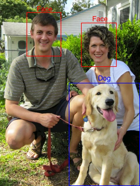
words. Experimental methods verify the computational
                                                               efficiency of K-means as opposed to EM. Our specific ap-
                                                               plication necessitates rapid training and image classifica-
                                                               tion, which precludes the use of the slower EM algorithm.

                                                               4     Learning Algorithms
                                                               Naive Bayes and Support Vector Machine (SVM) super-
                                                               vised learning algorithms are investigated in this paper.
                                                               The learning algorithms are used to classify an image
                                                               using the histogram vector constructed in the K-means
                                                               step.

Figure 1: Demonstration of how SURF feature vector is          4.1    Naive Bayes
built from image gradients.
                                                    A Naive Bayes classifier is applied to this BoW approach
                                                    to obtain a baseline classification system. The probability
open-source, MATLAB-optimized keypoint and descrip- φy=c that an image fits into a classification c is given by
tor extractor.                                                                    m
                                                                              1 X
                                                                    φy=c =           1{y (i) = c}.           (1)
                                                                             m i=1
3    K-means                                                Additionally, the probability φk|y=c , that a certain cluster
                                                            centroid, k, will contain a word count, xk , given that it
A key development in image classification using keypoints is in classification c, is defined to be
and descriptors is to represent these descriptors using a                        m
BoW model. Although spatial and geometric relation-                                                   (i)
                                                                                        1{y (i) = c}xk + 1
                                                                                    P
ship information between descriptors is lost using this as-
sumption, the inherent simplification gains make it highly             φk|y=c = i=1 m
                                                                                                              .      (2)
                                                                                    P       (i) = c}n
advantageous.                                                                           1{y            i   + N
                                                                                    i=1
   The descriptors extracted from the training images are
grouped into N clusters of visual words using K-means. Laplacian smoothing accounts for the null probabilities
A descriptor is categorized into its cluster centroid using of “words” not yet encountered. Using Equation 1 with
a Euclidean distance metric. For our purposes, we choose Equation 2, the classification of a query image is given
a value of N = 500. This parameter provides our model by
with a balance between high bias (underfitting) and high                                      Yn
                                                                                                         !
variance (overfitting).                                                    arg max φy=c           φi|y=c .            (3)
                                                                                 c
   For a query image, each extracted descriptor is mapped                                     i=1
into its nearest cluster centroid. A histogram of counts is
constructed by incrementing a cluster centroid’s number 4.2 SVM
of occupants each time a descriptor is placed into it. The
result is that each image is represented by a histrogram A natural extension to this baseline framework is to in-
vector of length N . It is necessary to normalize each his- troduce an SVM to classify the image based on its BoW.
togram by its L2-norm to make this procedure invariant Our investigation starts by considering an SVM with a
to the number of descriptors used. Applying Laplacian linear kernel
smoothing to the histogram appears to improve classifi-
cation results.                                                                 K(x, y) = xT y + c,                   (4)
   K-means clustering is selected over Expectation Max- due to its simplicity and computational efficiency in train-
imization (EM) to group the descriptors into N visual ing and classification. An intrinsic flaw of linear kernels

                                                           2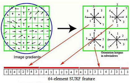
is that they are unable to capture subtle correlations be-
tween separate words in the visual dictionary of length
N.
To improve on the linear kernel’s performance, non-
linear kernels are considered in spite of their increased
complexity and computation time. More specifically the
χ2 kernel given by
n
X (xi − yi )2
K(x, y) = 1 − 2 , (5)
i=1
xi + yi
is implemented.
Given that an SVM is a binary classifier, and it is often
desirable to classify an image into more than two distinct
groups, multiple SVM’s must be used in conjunction to
produce a multiclass classification.
A one-vs-one scheme can be used in which a different Figure 2: Portrayal of one-vs-all SVM. When query image
SVM is trained for each combination of individual classes. is of type A, the A-vs-all SVM will correctly classify it.
An incoming image must be classified using each of these When the query image is not of class A, B, or C, it will
different SVM’s. The resulting classification of the image likely not be classified into any.
is the class that tallies the most “wins”. The one-vs-one
scheme involves making N2 different classifications for
N classes, which grows factorially with the number of the image correctly, and thus the overall output will place
classes. This scheme also suffers from false positives if the image into class A. When the query image is of a
an image is queried that does not belong to any of the different class, D, which is not already existent in the
classes. class structure, the query will always fall into the “all”
A more robust scheme is the one-vs-all classification class on the individual SVM’s. Hence, the query will not
system in which an SVM is trained to classify an image be falsely categorized into any class.
as either belonging to class c, or belonging to class ¬c. For It is important to reiterate that each multiclass SVM
m
the training data {(xi , yi )}i=1 , yi ∈ 1, ..., N , a multiclass only distinguishes between classes c and ¬c. A differ-
SVM aims to train N separate SVM’s that optimize the ent SVM is trained in this manner for each class. Thus,
dual optimization problem the number of SVM’s needed in a one-vs-all scheme only
grows linearly with the number of classes, N . This system
m m also does not suffer from as many false positives because
X 1 X (i) (j) images that do not belong to any of the classes are usually
max W (α) = αi − y y αi αj K(x(i) , x(j) ),
a
i=1
2 i,j=1 classified as such in each individual SVM.
(6) The specific multiclass SVM implementation used in
using John Platt’s SMO algorithm [3]. In Equation 6, this paper was MATLAB’s built-in version as described
K(x, z) corresponds to one of the Kernel functions dis- by Kecman [4].
cussed above.
A query image is then classified using
(m ) 5 Object Localization
X
(i) (i)
sgn αi y K(x , z) , (7) The methods described thus far are sufficient for the role
i=1
of classifying an image into a class when an object is
where sgn(x) is an operator that returns the sign of its prominently displayed in the forefront of the image. How-
argument and z is the query vector of BoW counts. ever, in the case when the desired object is a small subset
Figure 2 represents this concept visually. When the of the overall image, this object classification algorithm
query image is of class A, the A-vs-all SVM will classify will fail to classify it correctly. Additionally, there is mo-
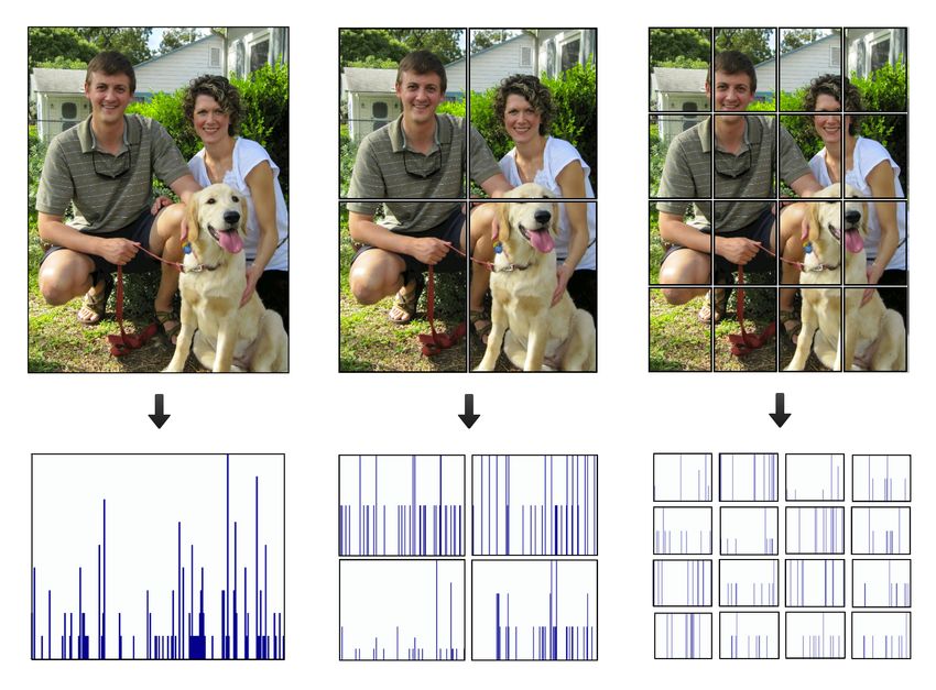
3Figure 3: Visual representation of partitioning an image Figure 4: Results showing both image classification and
into sub-images and constructing the histograms. localization.
tivation to localize an object in a scene using classification
The resulting effect is that pixel p is most highly influ-
techniques. The solution to these shortcomings is object
enced by the label of its lowest-level containing subsec-
localization using a hierarchical pyramid scheme. Figure
tion, in l = (L − 1), and less influenced by the label of its
3 illustrates the general idea behind extracting descrip-
highest-level containing subsection, in l = 0. The result-
tors using a pyramid scheme.
ing label given to pixel p can then be calculated as
First, the set of image descriptors, D, are extracted
from the image using SURF. Next, the image is seg-
labelpix (p) = arg max voteMap(c). (10)
mented into L pyramid levels, where L is a user-selected c
parameter that controls the granularity of the localiza-
tion search. Each level l, has subsections 0 ≤ i ≤ 4(l−1) ,
where 0 ≤ l ≤ (L − 1). At each level l, the entire set
6 Results and Future Work
of image descriptors, D, are segmented into a subgroup Figure 4 shows the classification and localization results
d ∈ D for section i which can be found as of our proposed algorithm on a generic image consisting
of multiple classes of objects.
" ! !# A more rigorous test of our method was done using
p.col − 1 p.row − 1 l a subset of the CalTech-101 database [5]. Images falling
i = idiv C
+ idiv R
2 + 1, (8)
2l 2 l into the four categories of airplanes, cars, motorbikes, and
faces were trained and tested using our method. Figure 5
for a given pixel p. The notation idiv(x) represents an shows the improvement in percent correct classifications
integer division operator. The symbols R and C are the in classification of Naive Bayes, linear SVM, and nonlin-
maximum number of rows and columns, respectively, in ear SVM as the training set size increases.
the original image. Then, for pixel p the votes at each The f -score, computed using the precision, P , and re-
level of the pyramid can be tallied into an N x1 map com- call, R, of the algorithm by
puted using
2P R
f= , (11)
P +R
L−1
(9) is perhaps a better indicator of performance because it
X
voteMap(c) = 2l−1 1{labelpyr (l, i) = c}.
l=0
is a statistical measure of a test’s accuracy. Figure 6
4Percent Correct vs. Training Set Size F Score vs. Training Set Size
90 1
Naive Bayes
Linear SVM
Non Linear SVM
85 0.95
Percent Correct
F Score
80 0.9
75 0.85
Naive Bayes
Linear SVM
Non Linear SVM
70
100 200 300 400 0.8
Training Set Size 100 200 300 400
Training Set Size
Figure 5: Percent correct classifications of supervised
Figure 6: f -score of classifications of supervised learning
learning classifiers.
classifiers.
shows a visible improvement in the f -score for all three opensurf.html, retrieved 11/04/2011.
classification algorithms as the training set size increases.
The nonlinear SVM maintains the largest f -score over [3] J. Platt. Sequential Minimal Optimization: A Fast
all training set sizes, which aligns with our hypothesized Algorithm for Training Support Vector Machines,
result. 1998.
Future work for this research should focus on replacing
K-means with a more robust clustering algorithm. One [4] V. Kecman. Learning and Soft Computing, MIT
option is Linearly Localized Codes (LLC) [6]. The LLC Press, Cambridge, MA. 2001.
method performs sparse coding on extracted descriptors [5] L. Fei-Fei, R. Fergus and P. Perona. Learning genera-
to make soft assignments that are more robust to local tive visual models from few training examples. CVPR,
spatial translations [7]. Furthermore, there is still open- 2004.
ended work to be done on the reconstruction of objects
using the individually labeled pixels from the pyramid lo- [6] J. Yang, K. Yu, Y. Gong, and T. Huang. Linear spa-
calization scheme. Hrytsyk and Vlakh present a method tial pyramid matching using sparse coding for image
of conglomerating pixels into their neighboring groups in classification. CVPR, 2009.
an optimal fashion [8].
[7] T. Serre, L. Wolf, and T.Poggio. Object recognition
with features inspired by visual cortex. CVPR, 2005.
References [8] N. Hrytsyk, V. Vlakh. Method of conglomerates
[1] D. Lowe. Towards a computational model for object recognition and their separation into parts. Methods
recognition in IT cortex. Proc. Biologically Motivated and Instruments of AI, 2009.
Computer Vision, pages 2031, 2000.
[2] C. Evans. Opensurf.
http://www.chrisevansdev.com/computer-vision-
5You can also read