Operation of the ATLAS trigger system in Run 2 - IOPscience
←
→
Page content transcription
If your browser does not render page correctly, please read the page content below
Journal of Instrumentation

Operation of the ATLAS trigger system in Run 2
To cite this article: The ATLAS collaboration 2020 JINST 15 P10004

View the article online for updates and enhancements.

                              This content was downloaded from IP address 46.4.80.155 on 11/12/2020 at 23:19
Published by IOP Publishing for Sissa Medialab
                                                                                                                       Received: July 27, 2020
                                                                                                                       Accepted: July 30, 2020
                                                                                                                    Published: October 2, 2020

Operation of the ATLAS trigger system in Run 2

                                                                                                                                                 2020 JINST 15 P10004
The ATLAS collaboration

   E-mail: atlas.publications@cern.ch

Abstract: The ATLAS experiment at the Large Hadron Collider employs a two-level trigger
system to record data at an average rate of 1 kHz from physics collisions, starting from an initial
bunch crossing rate of 40 MHz. During the LHC Run 2 (2015–2018), the ATLAS trigger system
operated successfully with excellent performance and flexibility by adapting to the various run
conditions encountered and has been vital for the ATLAS Run-2 physics programme. For proton-
proton running, approximately 1500 individual event selections were included in a trigger menu
which specified the physics signatures and selection algorithms used for the data-taking, and the
allocated event rate and bandwidth. The trigger menu must reflect the physics goals for a given data
collection period, taking into account the instantaneous luminosity of the LHC and limitations from
the ATLAS detector readout, online processing farm, and offline storage. This document discusses
the operation of the ATLAS trigger system during the nominal proton-proton data collection in
Run 2 with examples of special data-taking runs. Aspects of software validation, evolution of the
trigger selection algorithms during Run 2, monitoring of the trigger system and data quality as well
as trigger configuration are presented.

Keywords: Data acquisition concepts; Data reduction methods; Online farms and online filtering;
Trigger concepts and systems (hardware and software)

ArXiv ePrint: 2007.12539

                    c 2020 CERN for the benefit of the ATLAS collaboration. Published
                   by IOP Publishing Ltd on behalf of Sissa Medialab. Original content
from this work may be used under the terms of the Creative Commons Attribution 4.0             https://doi.org/10.1088/1748-0221/15/10/P10004
licence. Any further distribution of this work must maintain attribution to the author(s)
and the title of the work, journal citation and DOI.
Contents

1   Introduction                                     1

2   ATLAS detector                                   2

3   ATLAS trigger and data acquisition system        2

4   LHC fill cycle, fill patterns and ATLAS runs     5

                                                         2020 JINST 15 P10004
    4.1 The LHC fill cycle                           5
    4.2 LHC fill patterns in Run 2                   6
    4.3 Bunch groups                                 7
    4.4 The ATLAS run structure                      8

5   Operational model of the ATLAS trigger system    9

6   The Run-2 trigger menu and streaming model      10
    6.1 The trigger menu evolution in Run 2         11
    6.2 Cost monitoring framework                   11
    6.3 Run-2 streaming model                       12

7   Special data-taking configurations              13
    7.1 Runs with few bunches                       14
    7.2 Luminosity calibration runs                 16
    7.3 Enhanced bias runs                          17

8   Condition updates in the HLT                    17
    8.1 Conditions updates within a run             18
        8.1.1 Online beam spot                      18
        8.1.2 Online luminosity                     18
        8.1.3 Updates of trigger prescales          18
    8.2 Conditions update procedure                 19

9   Trigger configuration                           19
    9.1 The trigger database design                 20
    9.2 The TriggerTool                             21
    9.3 The TriggerPanel                            22
    9.4 Automatic prescaling of L1 trigger items    23

10 Online release validation                        23

11 Debug stream processing                          26

                                             –i–
12 Online monitoring                                                                                29
   12.1 Rate monitoring                                                                             29
   12.2 Online data quality monitoring                                                              30
   12.3 P-BEAST and shifter assistant                                                               31
   12.4 Data-taking anomalies                                                                       33

13 Offline monitoring and data quality assessment                                                   34

14 Conclusion                                                                                       36

                                                                                                          2020 JINST 15 P10004
The ATLAS collaboration                                                                             42

1   Introduction

The Trigger and Data Acquisition (TDAQ) system [1] is an essential component of the ATLAS
experiment [2] at the Large Hadron Collider (LHC) [3] as it is responsible for deciding in real time
whether to record data from a given collision. Its successful operation has a crucial impact on the
dataset used in physics analyses. The TDAQ system operated efficiently during the LHC Run 1
(2009–2013) [4] at instantaneous luminosities up to 8 × 1033 cm−2 s−1 and primarily at centre-of-
mass energies of 7 TeV and 8 TeV, collecting more than three billion proton-proton (pp) collision
events.
     In preparation for Run 2 (2015–2018), the TDAQ system underwent substantial upgrades
and modifications to cope with the challenging conditions expected for data-taking during those
years [4–6]. In Run 2, the higher instantaneous luminosities, which surpassed the original design
luminosity of 1034 cm−2 s−1 , as well as the larger number of interactions per bunch crossing, and
an increased centre-of-mass energy of 13 TeV led to a significant increase in the event rate from
interesting physics processes. In addition to pp collisions, the LHC provided heavy-ion collisions
at the end of each data-taking year. In 2015 and 2018, Pb+Pb collisions were recorded at a centre-
of-mass energy per nucleon of 5.02 TeV, in 2016 two datasets with p+Pb collisions were recorded at
5.02 TeV and 8.16 TeV, and in 2017 Xe+Xe collisions were recorded at 5.44 TeV. The operation of
the trigger system under these challenging pp data-taking conditions is described in this document.
     This paper is organised as follows. The ATLAS detector and TDAQ system is described in
sections 2 and 3. This is followed by a brief description of the LHC fill cycle, the fill patterns used
in Run 2 and a description of a typical ATLAS run in section 4. Section 5 introduces the ‘shifter
and expert’ model of the ATLAS trigger operations team. The following two sections, section 6 and
section 7, discuss the trigger selections for the nominal pp data-taking together with their evolution
during Run 2 and provide a few examples of special runs, respectively. Section 8 presents changes
of configuration and conditions that can be updated in real time during data-taking, while section 9
discusses the trigger configuration, database design and prescale mechanism. The validation
and sign-off cycle of the trigger software used during data-taking is described in section 10.
Section 11 discusses the debug stream, which contains events for which no decision could be made.
Two sections present the monitoring options available during data-taking (section 12), and the

                                                –1–
assessment of the quality of the fully reconstructed data (section 13). The conclusions are presented
in section 14.

2    ATLAS detector

The ATLAS detector [2] covers nearly the entire solid angle around the collision point.1 It consists
of an inner tracking detector surrounded by a thin superconducting solenoid, electromagnetic and
hadronic calorimeters, and a muon spectrometer incorporating three large superconducting toroidal
magnets.
     The inner-detector system is immersed in a 2 T axial magnetic field and provides charged-

                                                                                                                             2020 JINST 15 P10004
particle tracking in the range |η| < 2.5. The high-granularity silicon pixel detector covers the
vertex region and typically provides four measurements per track, the first hit being normally in
the insertable B-layer (IBL) installed before Run 2 [7, 8]. It is followed by the semiconductor
tracker (SCT) which usually provides eight measurements per track. These silicon detectors are
complemented by the transition radiation tracker (TRT), which enables radially extended track
reconstruction up to |η| = 2.0. The TRT also provides electron identification information based on
the fraction of hits above a higher energy-deposit threshold corresponding to transition radiation.
     The calorimeter system covers the pseudorapidity range |η| < 4.9. Within the region |η| < 3.2,
electromagnetic calorimetry is provided by barrel and endcap high-granularity lead/liquid-argon
(LAr) calorimeters, with an additional thin LAr presampler covering |η| < 1.8 to correct for
energy loss in material upstream of the calorimeters. Hadronic calorimetry is provided by the
steel/scintillator-tile calorimeter, segmented into three barrel structures within |η| < 1.7, and two
copper/LAr hadronic endcap calorimeters. The solid angle coverage is completed with forward
copper/LAr and tungsten/LAr calorimeter modules optimised for electromagnetic and hadronic
measurements respectively.
     The muon spectrometer (MS) uses separate trigger and high-precision tracking chambers to
measure the deflection of muons in a magnetic field generated by the superconducting air-core
toroids. The field integral of the toroids ranges between 2.0 and 6.0 T m across most of the detector.
A set of precision tracking chambers covers the region |η| < 2.7 with three layers of monitored
drift tubes, complemented by cathode-strip chambers (CSCs) in the forward region where the
background is highest. The muon trigger system covers the range |η| < 2.4 with resistive-plate
chambers (RPCs) in the barrel, and thin-gap chambers (TGCs) in the endcap regions.

3    ATLAS trigger and data acquisition system

The ATLAS TDAQ system is responsible for online processing, selecting and storing events of
interest for offline analysis, and is shown diagrammatically in figure 1. Events are selected using a
two-stage trigger system [5].
   1ATLAS uses a right-handed coordinate system with its origin at the nominal interaction point (IP) in the centre of the
detector and the z-axis along the beam pipe. The x-axis points from the IP to the centre of the LHC ring, and the y-axis
points upwards. Cylindrical coordinates (r, φ) are used in the transverse plane, φ being the azimuthal angle around the
z-axis. The pseudorapidity
               q            is defined in terms of the polar angle θ as η = − ln tan(θ/2). Angular distance is measured in
units of ∆R ≡   (∆η)2 + (∆φ)2 .

                                                         –2–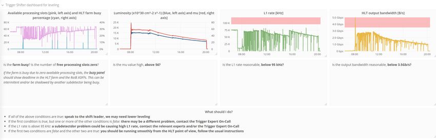
Calorimeter detectors
                                      TileCal      Muon detectors

                                                                                                                 Detector
     Level-1 Calo                                   Level-1 Muon                                                 Read-Out
              Preprocessor                     Endcap           Barrel
                                             sector logic     sector logic                      FE      FE    ...    FE

       CP (e,γ,τ)    JEP (jet, E)
                                                                                                ROD    ROD           ROD

                                                                               Level-1 Accept
                                                       Muon CTP
                                                        Interface
                                                       (MUCTPI)

                                                                                                                            2020 JINST 15 P10004
                                                                                                      DataFlow
                                    L1Topo
                                                                                                Read-Out System (ROS)
                                                                Central
                                                                Trigger
                                                               Processor
                                                                 (CTP)

                                                                                  Pixel/SCT
                                                     Central Trigger
  Level-1
                                                                                                Data Collection Network
                                             RoI            Fast TracKer
                                                               (FTK)

                                                   High Level Trigger
                                                         (HLT)
                                                                                                      Data Storage
                                                                  Accept
                                                      Processors
                                                                             Event
                                                                             Data                       Tier-0

Figure 1. The ATLAS TDAQ system in Run 2 showing the components relevant for triggering as well as the
detector read-out and data flow.

     The Level-1 (L1) trigger is a hardware-based system that uses custom electronics to trigger on
reduced-granularity information from the calorimeter and muon detectors [9]. The L1 calorimeter
(L1Calo) trigger takes signals from the calorimeter detectors as input [10]. The analogue detector
signals are digitised and calibrated by the preprocessor, and sent in parallel to the Cluster Processor
(CP) and Jet/Energy-sum Processor (JEP). The CP system identifies electron, photon, and τ-lepton
candidates above a programmable threshold, and the JEP system identifies jet candidates and
produces global sums of total and missing transverse energy. The signals from the LAr calorimeter
are bipolar and span multiple bunch crossings, which introduces a dependence of the amplitude on
the number of collisions occurring in neighbouring bunch crossings (out-of-time pile-up). Objects
with narrow clusters such as electrons are not strongly affected by small shifts in energy, however the
missing transverse momentum is very sensitive to small systematic shifts in energy over the entire
calorimeter. These effects are mitigated in the L1Calo trigger by a dedicated pedestal correction
algorithm implemented in the firmware [11].
     The L1 muon (L1Muon) trigger uses hits from the RPCs (in the barrel) and TGCs (in the end-
caps) to determine the deviation of the hit pattern from that of a muon with infinite momentum [12].
To reduce the rate in the endcap regions of particles not originating from the interaction point, the
L1Muon trigger applies coincidence requirements between the outer and inner TGC stations, as
well as between the TGCs and the tile calorimeter.

                                                             –3–
The L1 trigger decision is formed by the Central Trigger Processor (CTP), which receives
inputs from the L1Calo trigger, the L1Muon trigger through the L1Muon Central Trigger Processor
Interface (MUCTPI) and the L1 topological (L1Topo) trigger [13] as well as trigger signals from
several detector subsystems such as the Minimum Bias Trigger Scintillators (MBTS) [14], the
LUCID Cherenkov counter [15] and the zero-degree calorimeter (ZDC) [16].
     The CTP is also responsible for applying dead time, which is a mechanism to limit the number
of L1 accepts to be within constraints on detector read-out latency [17]. This preventive dead
time limits the minimum time between two consecutive L1 accepts (simple dead time) to avoid
overlapping read-out windows, and restricts the number of L1 accepts allowed in a given number of
bunch crossings (complex dead time) to prevent front-end buffers from overflowing. The complex

                                                                                                        2020 JINST 15 P10004
dead time uses a leaky bucket model to emulate a front-end buffer. In this model, dead time is
applied when the bucket is full. The size of the bucket is X, expressed in units of L1 accepts and
R (in units of bunch crossings), the time it takes to read out one L1 accept. With these numbers
the trigger rate, on average, is limited to X triggers in a time period of X × R bunch crossings.
At the end of Run 2, the simple dead time setting was four bunch crossings, which corresponds
to an inefficiency of about 1% for a L1 rate of 90 kHz. The complex dead time was configured
with four different leaky bucket algorithms and one sliding-window algorithm to cover the read-out
limitations of the various sub-detectors. The total peak inefficiency was about 1% for a L1 rate
of 90 kHz.
     The L1 trigger can select events by considering event-level quantities (e.g. the total energy
in the calorimeter), the multiplicity of objects above thresholds (e.g. the transverse momentum
of a muon, etc.), or by considering topological requirements (such as invariant masses or angular
distances). The topological requirements are applied in the L1Topo trigger to geometric or kinematic
combinations between trigger objects received from the L1Calo or L1Muon systems. The L1 trigger
accepts events at a rate up to the maximum detector read-out rate of 100 kHz, down from the bunch
crossing rate of about 40 MHz, within a latency of 2.5 µs.
     For each L1-accepted event, the Front-End (FE) detector electronics read out the event data for
all detectors. The data are sent first to ReadOut Drivers (RODs), performing the initial processing
and formatting, and then to the ReadOut System (ROS) to buffer the data. The data from the
different sub-detectors are sent from the ROS to the second stage of the trigger, the High-Level
Trigger (HLT), only when requested by the HLT. In addition to performing the first selection step,
the L1 triggers identify Regions-of-Interest (RoIs) in η and φ within the detector to be investigated
by the second trigger stage.
     The second stage of the trigger, the HLT, is software-based. A typical reconstruction sequence
makes use of dedicated fast trigger algorithms to provide early rejection, followed by more precise
and more CPU-intensive algorithms that are similar to those used for offline reconstruction to make
the final selection. These algorithms are executed on a dedicated computing farm of approximately
40 000 selection applications known as Processing Units (PUs). Between each year of data taking,
older hardware in the farm was replaced with newer hardware on a rolling basis to increase
the available computing power and the total number of PUs. The PUs are designed to make
decisions within a few hundred milliseconds. A step in such a sequence of algorithms will typically
execute one or multiple feature-extraction algorithms requesting event-data fragments from within
an RoI and terminate on a hypothesis algorithm which uses the reconstructed features to decide

                                               –4–
whether the trigger condition is satisfied or not. In some cases, information from the full detector is
requested in order to reconstruct physics objects (e.g. for the reconstruction of the missing transverse
momentum [18]). The HLT software is largely based on the offline software Athena [19], which
itself is based on Gaudi [20], a framework for data processing for HEP experiments. Gaudi/Athena
is a component-based framework where each component (e.g. algorithm, service, tool) is configured
by a set of properties that can be defined during the configuration stage of the application. The
physics output rate of the HLT during an ATLAS data-taking run (see section 4.4) is on average
1.2 kHz with an average physics throughput to permanent storage of 1.2 GB/s. Once an event is
accepted by the HLT, the Sub-Farm Output (SFO) sends the data to permanent storage for offline
reconstruction and exports the data to the Tier-0 facility [21] at CERN’s computing centre.

                                                                                                           2020 JINST 15 P10004
      The Fast TracKer (FTK) [22] is a hardware-based system for inner-detector track reconstruction
designed to provide tracks to the HLT at the L1 accept rate. It was undergoing commissioning
during Run 2 and was not used by the HLT for trigger decisions.

4     LHC fill cycle, fill patterns and ATLAS runs

In the following, the LHC fill cycle, the fill pattern and their representation in ATLAS, the so-called
bunch groups, are described. Additionally, the ATLAS run, which refers to a continuous period of
data acquisition that typically corresponds to an LHC fill cycle, is laid out.

4.1    The LHC fill cycle
The LHC is a circular particle accelerator that is the last in a chain of accelerators used to bring
particle beams into collisions at their final energies. The beams travel through the LHC in opposite
directions in separate rings of superconducting magnets, which are crossed at four interaction points.
The beams are kept separated in the interaction points using magnetic fields until they are ready
for collisions. The LHC aims to provide the largest, usable integrated luminosity of high-energy
proton and ion collisions to the LHC experiments. To provide collisions to the experiments, the
LHC has to go through a cycle composed of several phases [23], which are shown in figure 2. Each
phase refers to one or several beam modes and all together are referred to as the nominal cycle:

      • Injection: after the current in the magnets is increased to provide the field necessary for
        injection, beams are injected from the accelerator chain into the LHC rings following a filling
        scheme, specifying the number of proton bunches and the spacing between them.

      • Ramp: the beams are accelerated to the collision energy. During this phase, the radio
        frequency systems accelerate the particles and the current in the magnets is further increased.

      • Squeeze and adjust: in these two phases, beams are prepared for collisions. First, the beam
        sizes at the interaction points are reduced (squeeze), then the beams are adjusted so that they
        are optimally colliding (adjust).

      • Stable beams: this is the phase when the LHC conditions are stable, collisions take place in
        the experiments, and it is safe for detectors to be turned on to record data. Small adjustments
        of beam parameters are permitted [24, 25]. The LHC spent approximately 50% of the time
        in stable beams throughout Run 2.

                                                 –5–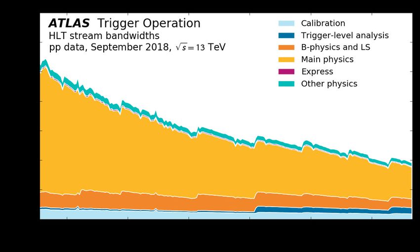
Field in main magnets          Beam 1 intensity (current)         Beam 2 intensity (current)

                                                         6.5 TeV

         450 GeV

                                                                                                                                      2020 JINST 15 P10004
                                                                                                                               Time
               Injection                    Ramp       Squeeze              Stable Beams for Physics                 Dump &
                                                       & Adjust                                                    Ramp Down

Figure 2. The LHC goes through a cycle composed of several phases: the injection of beams into the rings,
the acceleration to the collision energy during ramp, the preparation of beams for collisions during squeeze
and adjust, the phase where collisions take place during stable beams, the extraction of the beams from the
rings during dump, and finally the ramping down of the magnetic fields. Adapted from ref. [27].

      • Dump and ramp down: beams are extracted from the rings and safely dumped. The dump can
        either be planned (by the LHC), requested (for example by experiments in case of problems
        with the detector) or unplanned. Following the dump, the magnetic fields are ramped down.

The time in between two consecutive stable beams periods is referred to as turnaround, and
includes the nominal cycle as well as all necessary actions to set up the machine for operation with
beams. The ideal duration of the stable beams phase is typically 10–15 hours, depending on several
factors, including luminosity lifetime, average turnaround duration, and predicted availability of the
machine.
     In about every second fill in the last year of Run 2, fast luminosity scans were performed [26]
during stable beams to provide feedback on the transverse emittance at a bunch-by-bunch level to
the LHC. During these scans, beams are offset against each other in the x- and y-plane in several
displacement steps. The scans were typically done a few minutes after stable beams had been
declared and just before the end of the stable beams period, and lasted a few minutes.

4.2    LHC fill patterns in Run 2
During Run 2, the LHC machine configuration evolved significantly. This was a major factor in
improving luminosity performance each year of Run 2 [28]. The various bunch filling patterns
used have a direct impact on the trigger configuration. With the changing running conditions,
adjustments had to be made in order to respect the trigger and DAQ system limitations (see e.g.
section 7.1).
     At the start of Run 2 in 2015, the LHC used 50 ns bunch spacing and switched in August 2015 to
the nominal 25 ns bunch spacing scheme [29]. In June 2016, the high-brightness version of the 25 ns
beam obtained through the Batch Compression, Merging and Splitting (BCMS) scheme [30] became
operational for physics production. These changes brought about an increase in instantaneous
luminosity to about 1.3 × 1034 cm−2 s−1 , resulting in higher trigger rates and an evolution in the

                                                                        –6–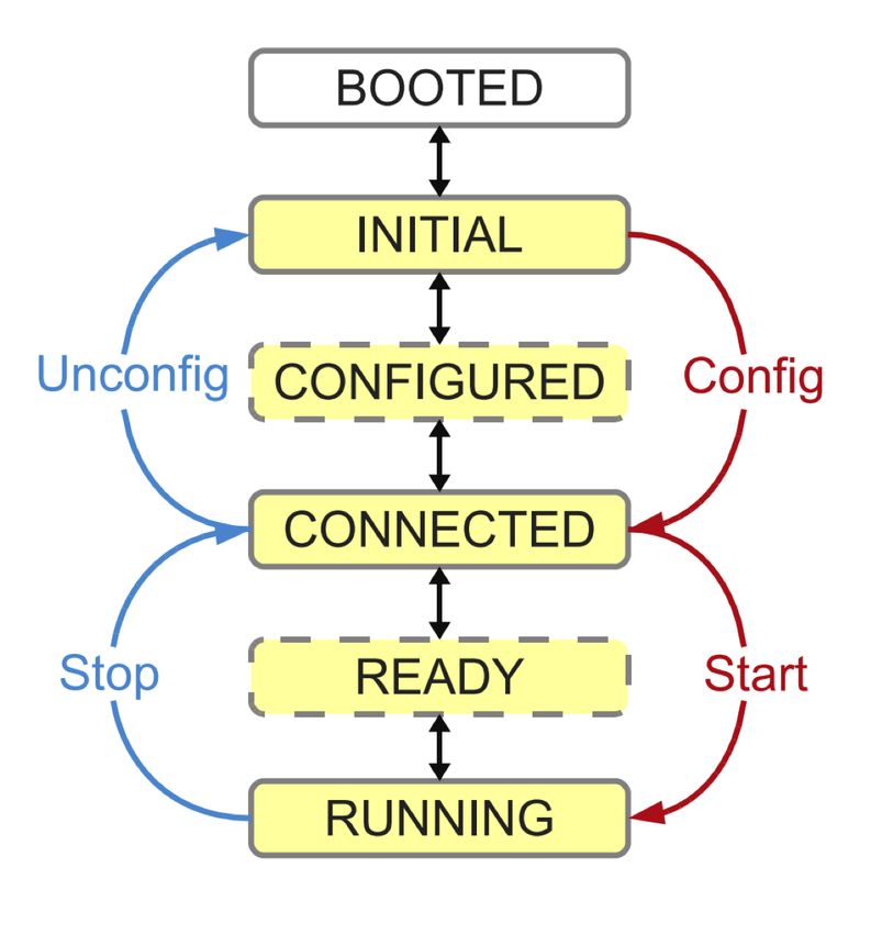
ATLAS Trigger Operation

Figure 3. Example bunch group configurations for four out of the 16 possible bunch groups. The numbers
in blue on the right indicate the number of bunch crossings for each group. The group of the bunch counter
reset veto (BCRVeto) leaves a short time slice for distribution of the LHC bunch counter reset signal to the on-
detector electronics. The Paired bunch group indicates the bunch crossing IDs with colliding bunches, while

                                                                                                                   2020 JINST 15 P10004
the Empty bunch group contains no proton bunches and is generally used for cosmic ray, noise and calibration
triggers. The calibration requests (CalReq) bunch group can be used to request calibration triggers.

trigger strategy. In 2017, several LHC fills were dumped because of beam losses in the LHC
sector 16L2 [31]. As a consequence, the 8b4e filling scheme [32] (eight bunches with protons,
four bunches without protons) and later its high-brightness variant 8b4e BCS (Batch Compression
and Splitting) with their low e-cloud build-up characteristics were made operational. The 8b4e
filling schemes circumvented the problem, but resulted in a reduction in the number of colliding
bunches by 30% compared to the BCMS scheme. To compensate for the loss in luminosity due to
the decrease in colliding bunches, the bunch intensity was increased and this led to a 33% increase
of simultaneous interactions per bunch crossing (‘pile-up’), up to 80 interactions compared to
up to 60 interactions previously. Such an increase together with the high luminosities of up to
1.9 × 1034 cm−2 s−1 [33] would have resulted in an increase of trigger rates, straining the CPU
resources of the HLT farm. The trigger configuration intended to be used for a luminosity of up to
2.0 × 1034 cm−2 s−1 with a pile-up of 60 would have required higher trigger thresholds at a pile-up
of 80, leading to a reduced efficiency for many physics analyses. Therefore, ATLAS requested that
the luminosity be kept constant for the first few hours of a run (luminosity-levelling) at a luminosity
of 1.56 × 1034 cm−2 s−1 with a pile-up of 60. In 2018, the LHC switched back to the 25 ns BCMS
beam for luminosity production, as the problems with beam losses in 16L2 were mitigated [34],
and the pile-up interactions were again reduced to about 60. More information about these filling
schemes can be found in ref. [32].

4.3    Bunch groups

In the LHC, there are a total of 3564 bunch crossings per LHC revolution. Each of these bunch
crossings can have either two bunches colliding, one bunch, or be empty of protons. Each bunch
crossing is identified by a Bunch Crossing Identifier (BCID) from 0 to 3563. A list of BCIDs is
called a bunch group.
     Bunch group conditions are used in combinatorial logic ‘AND’ with other trigger conditions
to define which items generate a L1 accept. There are 16 distinct bunch groups that can be defined
in ATLAS, each with its own particular purpose, defined for each LHC bunch. Figure 3 shows four
types of bunch groups which are described in the following.
     Bunch group conditions can be paired (colliding) bunches for physics triggers, single (one-
beam) bunches for background triggers and empty bunches for cosmic ray, noise and calibration

                                                     –7–
triggers. More complex schemes are possible, e.g. requiring unpaired bunches separated by at least
75 ns from any bunch in the other beam. Two bunch groups have a more technical purpose: the
calibration requests group defines the times at which sub-detectors may request calibration triggers,
typically in the long gap with no collisions and the group of the bunch counter reset veto leaves a
short time slice for distribution of the LHC bunch count reset signal to the on-detector electronics.
As the LHC filling scheme can vary from fill to fill, ATLAS has developed and commissioned
a procedure for monitoring and redefining the bunch groups using dedicated electrostatic detectors.
These so-called beam pick-ups [35] are located 175 m upstream of the interaction point. An online
application measures the filling scheme seen by the beam pick-ups and calculates the corresponding
bunch groups. While the configuration of some bunch groups is given by the LHC (e.g. the colliding
2020 JINST 15 P10004
BCIDs) through the fill pattern, others can be defined to contain any desired list of BCIDs for specific
data-taking requests (e.g. in van der Meer scans [33] or single-beam background studies).
The 16 bunch group configurations are together called a bunch group set, which is different for
each different LHC filling scheme. The bunch group sets are generated for each filling scheme in
advance of running, using information about the positions of bunches with protons in each beam
provided by the LHC. The generated bunch group set is then checked against the measured beam
positions to ensure that it matches. The CTP pairs each L1 trigger item with a specific bunch group
defined in the set. Those L1 trigger items which are employed to select events for physics analyses
trigger on bunch groups containing all colliding BCIDs. The CTP can also provide random triggers
and apply specific bunch crossing requirements to those.
4.4 The ATLAS run structure
An ATLAS run is a period of data acquisition with stable detector configuration and in the case
of physics data-taking usually coincides with an LHC fill, which can last many hours. Another
example is a cosmic-ray data-taking run, which takes place when there is no beam in the LHC and
the ATLAS detector is used to detect cosmic rays to study detector performance [36]. The DAQ
system assigns a unique number to every run at its beginning. An identifier is assigned to each
event and is unique within the run (starting at 0 for each run). A run is divided into Luminosity
Blocks (LB), with a length of the order of one minute and identified by an integer unique within a
given run. A LB defines an interval of constant luminosity and stable detector conditions (including
the trigger system and its configuration). To define a data sample for physics, quality criteria are
applied to select LBs where conditions are acceptable. The instantaneous luminosity in a given LB
is multiplied by the LB duration to obtain the integrated luminosity delivered in that LB. The length
of the LB can be changed during the run and a new LB can be started at any time (following a 10
second minimum delay). From a data quality point of view, the LB represents the smallest quantity
of data that can be declared good or bad for physics analysis.
To start a run, the software and hardware components of the ATLAS detector have to follow the
transitions of a finite-state machine [37]. The transitions performed by the applications are shown in
figure 4. During ‘boot’, all applications are being started. In the ‘configure’ and ‘connect’ transitions,
the hardware and applications are configured and connections between different applications are
established where necessary. Finally, during ‘start’, a run number is assigned and the applications
perform their final (run-dependent) configuration. Once all applications arrived at the ‘ready state’,
the CTP releases the inhibit and events start flowing through the system.
–8–2020 JINST 15 P10004
Figure 4. The software and hardware components of the ATLAS detector follow the transitions of a
finite-state machine used to synchronise the configuration of all applications and detectors within ATLAS.
Run-dependent configurations (e.g. loading of conditions data) are performed during the start transition,
which can take several minutes for the entire ATLAS detector [37].
5 Operational model of the ATLAS trigger system
During the operation of the LHC, the ATLAS detector is operated and monitored by a shift crew
in the ATLAS control room (ACR), 24 hours a day, 7 days a week, supported by a pool of remote
on-call experts. Shifters and experts are responsible for the efficient collection of high-quality data.
The operation and data quality monitoring of the trigger system is overseen by two operation
coordinators whose main responsibility is to ensure smooth and efficient data-taking. They coordi-
nate a team of weekly on-call experts, on rotation, for the areas listed below. Operation coordinators
and on-call experts work together closely at a daily trigger operation meeting to plan the activities
of the day.
• ACR trigger desk: during the shift in the ACR, the person is responsible for providing the
needed trigger configuration and for monitoring the operation of the trigger system in close
communication with other ACR shifters.
• Online: responsible for the proper operation of the ATLAS trigger and primary support for
the ACR trigger shifter.
• Trigger menu: responsible for the preparation of the trigger configuration of active triggers
and their prescale factors (see section 6).
• Online release: collection and review of software changes and monitoring the state of the
software release for online usage via validation tests that run every night; deployment of the
online software release on the machines used during data-taking.
• Reprocessing: in charge of validating the online software release (see section 10) by running
the simulation of the L1 hardware and the HLT software on a dedicated dataset to spot errors
by running on large samples.
• Data quality and debug stream: responsible for the data quality assessment of recorded data;
investigate and recover the events in the debug stream (see section 11).
–9–• Signature-specific: monitor the performance of triggers for signatures, assist in data quality
assessment and reprocessing sign-off; several trigger signatures are grouped together (muon
and B-physics and Light States; jet, missing transverse momentum and calorimeter energy
clusters; τ-lepton, electron and photon; b-jet signature and tracks).
• Level-1: each L1 trigger system (L1Calo, L1Muon barrel, L1Muon endcap, and CTP) has an
on-call expert who helps to ensure smooth operation of the L1 trigger and monitors the data
quality for their respective system.
In additon to data-taking, the trigger operation group participates in special runs of a technical
nature together with the ATLAS DAQ team to develop and test the online software and tools
2020 JINST 15 P10004
to be used for data-taking. It also provides support for other ATLAS systems during detector
commissioning runs and for special tests during LHC downtime periods.
6 The Run-2 trigger menu and streaming model
Events are selected by trigger chains, where a chain consists of a L1 trigger item and a series of
HLT algorithms that reconstruct physics objects and apply kinematic selections to them. Each chain
is designed to select a particular physics signature such as the presence of leptons, photons, jets,
missing transverse momentum, total energy and B-meson candidates. The list of trigger chains used
for data-taking is known as a trigger menu, which also includes prescales for each trigger chain.
To control the rate of accepted events, a prescale value, or simply prescale, can be applied. For a
prescale value of n, an event has a probability of 1/n to be kept. Individual prescale factors can be
given to each chain at L1 or at the HLT, and can be any value greater than or equal to one. More
details of how prescales are applied can be found in section 8.1.3.
The complete set of trigger selections must respect all trigger limitations and make optimal
use of the available resources at L1 and the HLT (e.g., maximum detector read-out rate, available
processing resources of the HLT farm, and maximum sustainable rate of permanent storage). Rates
and resource usage are determined as described in section 6.2 and section 7.3.
The configuration is driven by the physics priorities of the experiment, including the number of
clients satisfied by a particular trigger chain. The main goal of the Run-2 trigger menu design was
to maintain the unprescaled single-electron and single-muon trigger pT thresholds around 25 GeV
despite the expected higher trigger rates to ensure the collection of the majority of events with
leptonic W and Z boson decays. The primary triggers (used for physics analyses and unprescaled)
cover all signatures relevant to the ATLAS physics programme including electrons, photons, muons,
τ-leptons, jets, b-jets and ET which are used for Standard Model precision measurements including
decays of the Higgs, W and Z bosons, and searches for physics beyond the Standard Model such
as heavy particles, supersymmetry or exotic particles. A set of low transverse momentum dimuon
triggers is used to collect B-meson decays, which are essential for the B-physics programme of
ATLAS.
Heavy-ion (HI) collisions differ significantly from pp collisions, and therefore require a ded-
icated trigger menu to record the data. The main components of the HI trigger menu are triggers
selecting hard processes (high ET , b-jets, muons, electrons, and photons) in inelastic Pb+Pb col-
lisions, minimum-bias triggers for peripheral and central collisions, triggers selecting events with
– 10 –particular global properties (event-shape triggers to collect events with large initial spatial asymme-
try of the collisions, ultra-central collision triggers), as well as triggers selecting various signatures
in ultra-peripheral collisions. More information about the HI trigger menu and associated streams
can be found in ref. [38].
Apart from the trigger menu used to record nominal pp or HI collisions, additional trigger
menus were designed in Run 2 for special data-taking configurations, with some examples discussed
in section 7.
6.1 The trigger menu evolution in Run 2
The trigger menu for pp data-taking evolved throughout Run 2 due to the increase of the instanta-
2020 JINST 15 P10004
neous luminosity and the number of pile-up interactions. The composition of the trigger menu is
developed based on the expected luminosity for each year, with looser selections deployed during
early data-taking or when the peak luminosity falls below the predicted target value. The main
trigger chains that comprise the ATLAS trigger menu for 2015 targeting an instantaneous luminosity
of 5 × 1033 cm−2 s−1 and valid for a peak luminosity up to 6.5 × 1033 cm−2 s−1 are described in detail
along with their performance in ref. [39]. As the instantaneous luminosity increased substantially in
2016 (up to 1.3 × 1034 cm−2 s−1 ) and again in 2017 (up to 1.6 × 1034 cm−2 s−1 ), it became necessary
to adjust the trigger menu each year accordingly. The various improvements and the performance
for the trigger menu used in 2016 and 2017 are described in detail in refs. [40] and [38], respectively.
The peak luminosity in 2018 was close to 2.0 × 1034 cm−2 s−1 . Even though the luminosity was
higher than in 2017, the number of interactions per bunch crossing was similar. The resources
needed to continue running the same trigger menu as in 2017 were estimated to fall within the
limitations of the trigger system. The 2018 trigger menu [41] therefore only contained additions on
top of the 2017 menu together with a few changes and improvements to the trigger selections used
in 2017.
6.2 Cost monitoring framework
The ATLAS cost monitoring framework [42] consists of a suite of tools to collect monitoring data
on both CPU usage and data-flow over the data-acquisition network during the trigger execution.
These tools are executed on a sample of events processed by the HLT, irrespective of whether the
events pass or fail the HLT selection. It is primarily used to prepare the trigger menu for physics
data-taking through the detailed monitoring of the system, allowing data-driven predictions to be
made utilising dedicated datasets (enhanced bias dataset, see section 7.3). Monitored data include
algorithm execution time, data request size, and the logical flow of the trigger execution for all L1-
accepted events. To sample a representative subset of all L1-accepted events, a monitoring fraction
of 10% is chosen. Example monitoring distributions are given for two of the many algorithms in
figure 5: calorimeter topological clustering [43] and electron tracking. These monitoring data were
collected over a 180 s data-taking period at 1 × 1034 cm−2 s−1 . Topological clustering can run either
within an RoI or as a full detector scan, leading to a double-peak structure in the processing time as
shown in figure 5 (top left). Equivalently to the procedure of predicting the rates of individual HLT
chains and trigger menus (see sections 7.3 and 10), it is possible to estimate the number of HLT
PUs which will be required to run a given trigger chain or menu. This functionality was extremely
useful in planning for different LHC scenarios in 2017 and in preparation for 2018 data-taking.
– 11 –Events
Events
TrigCaloClusterMaker_topo 106 TrigCaloClusterMaker_topo
106 TrigFastTrackFinder_Electron_IDTrig TrigFastTrackFinder_Electron_IDTrig
105
105
s = 13 TeV s = 13 TeV
104
104 ATLAS ATLAS
103 103
102 102
10 10
0 50 100 150 200 250 300 350 400 450 500 0 200 400 600 800 1000 1200
Time Per Call [ms] Time Per Event [ms]
2020 JINST 15 P10004
×103
Events
106
Events
TrigCaloClusterMaker_topo
TrigCaloClusterMaker_topo TrigFastTrackFinder_Electron_IDTrig
250 TrigFastTrackFinder_Electron_IDTrig
105
200
s = 13 TeV
s = 13 TeV 104
ATLAS
ATLAS
150
103
100
102
50
10
0.1 0.2 0.3 0.4 0.5 0.6 0.7 0.8 5 10 15 20 25
Fractional Time Per Event Calls Per Event
Figure 5. Cost monitoring distributions for two HLT algorithms [42]: the topological clustering of calorime-
ter data (TrigCaloCluserMaker_topo) is shown in green and the inner-detector electron track identification
(TrigFastTrackFinder_Electron_IDTrig) is shown in red. Presented are the execution time (top) per call
(left) and per event (right), as well as the execution time expressed as a fraction of the total execution time
of all algorithms (bottom) in the event (left) and number of executions per event (right). Only statistical
uncertainties are shown.
6.3 Run-2 streaming model
The trigger menu defines the streams to which an event is written, depending on the trigger chains
that accepted the event. Data streams are subdivided into files for each luminosity block, which
facilitates the subsequent efficiency and calibration measurements under varying running conditions.
The five different types of data streams considered in the recording rate budget available at the
HLT during nominal pp data-taking are:
• Physics stream: contains events with collision data of interest for physics studies. The events
contain full detector information and dominate in terms of processing, bandwidth and storage
requirements.
• Express stream: very small subset of the physics stream events reconstructed offline in real
time for prompt monitoring and data quality checks.
• Debug streams: events for which no trigger decision could be made are written to this stream.
These events need to be analysed and recovered separately to identify and fix possible problems
in the TDAQ system (see section 11).
– 12 –• Calibration streams: events which are triggered by algorithms that focus on specific sub-
detectors or HLT features are recorded in these types of streams. Depending on the purpose
of the stream, only partial detector information is recorded through a strategy called Partial
Event Building (PEB) [5], which has the potential to significantly reduce the event size.
• Trigger-Level Analysis (TLA) streams: events sent to this stream store only partial detector
information and specific physics objects reconstructed by the HLT to be used directly in a
physics analysis.
• Monitoring streams: events are sent to dedicated monitoring nodes to be analysed online for,
2020 JINST 15 P10004
e.g., detector monitoring, but are not recorded.
For special data-taking configurations it is possible to introduce additional streams; an example
is the recording of enhanced bias data, which is discussed in section 7.3. With the exception of
the debug streams, the streaming model is inclusive, which means that an event can be written
to multiple streams. Aside from the express stream, there are typically multiple different streams
of each type. For PEB, data are only stored for specific sub-detectors, or for specific regional
fragments from specific sub-detectors. Similarly, the TLA stream (see ref. [44] for more details of
the procedures) only stores physics objects reconstructed by the HLT with limited event information
and uses these trigger-level objects directly in a physics analysis [45]. By writing out only a fraction
of the full detector data, the event size is reduced, making it possible to operate these triggers at
higher accept rates while not being limited by constraints on the output bandwidth. This strategy is
effective in avoiding high prescales at the HLT for low transverse momentum (pT ) triggers.
Figure 6 shows the average recording rate of the physics data streams of all ATLAS pp runs
taken in 2018. Events for physics analyses are recorded at an average rate of ∼1.2 kHz. This
comprises two streams, one dedicated to B-physics and Light States (BLS) physics data, which
averaged 200 Hz, and one for all other main physics data, which averaged the targeted 1 kHz. The
BLS data are kept separate so the offline reconstruction can be delayed if available resources for
processing are scarce.
Figure 7 shows the HLT rates and output bandwidth as a function of time in a given run. The
apparent mismatch between rate and output bandwidth in some streams is due to the use of PEB
techniques. The increase of the TLA HLT output is part of the end-of-fill strategy of the ATLAS
trigger. Towards the end of the LHC fill, when the luminosity and the pile-up are reduced compared
to their peak values, L1 bandwidth and CPU resources are available to record and reconstruct
additional events using lower-threshold TLA trigger chains.
Table 1 shows the average event sizes for the described streams. The event size of physics,
express and BLS streams is comparable whereas the TLA stream event size is significantly smaller.
The calibration stream size varies considerably depending on the purpose and what sub-detector
information is written out.
7 Special data-taking configurations
In addition to standard pp and heavy-ion data-taking, the LHC programme includes a variety
of short periods when the machine is operated with particular beam parameters, referred to as
– 13 –Table 1. The average event sizes for the physics and express stream, the trigger-level analysis, calibration
and B-physics and Light States (BLS) are presented in this table.
Stream Average event size
Physics, express 1 MB
Trigger-level analysis 6.5 kB
Calibration 1.3 kB to 1 MB
B-physics and light states 1 MB
Average rate per run [Hz]
2500 Physics Main
ATLAS Trigger Operation
2020 JINST 15 P10004
B Physics and Light States
Average total rate (1.2 kHz) Data 2018, s = 13 TeV, p-p runs
2000 Average rate Physics Main (1.0 kHz)
1500
1000
500
0
April May June July August September October
Date of run
Figure 6. The average recording rate of the main physics data stream and the BLS data stream for each
ATLAS pp physics run taken in 2018. The average of all runs for these two streams is indicated as a red
dash-dotted line, and the average of the main physics stream is indicated as a blue dashed line.
special data-taking configurations. The special data-taking configurations provide data for detector
and accelerator calibration as well as additional physics measurements in the experiments. The
specific LHC bunch configurations and related conditions (e.g. lower number of paired bunches,
change in the average number of pile-up interactions), detector settings (e.g. subsystem read-out
settings optimised for collecting calibration data) and desired trigger configuration have to be taken
into account when preparing the trigger menu. The preparation of these configurations can be
quite extensive as they require a specific trigger menu which needs to be prepared and adjusted to
comply with the imposed, usually tightened limits in rate, bandwidth and CPU consumption. In
the following, three examples of special data-taking configurations, and the challenges that come
with them, are discussed: runs with a low number of bunches, luminosity calibration runs and a
configuration used to record enhanced minimum-bias data for future estimates of trigger rates and
CPU consumption.
7.1 Runs with few bunches
Runs with a low number of bunches (e.g. 3, 12, 70, 300 bunches) usually occur during the periods
of intensity ramp-up of the LHC after long or end-of-year shutdowns [46]. While in most of these
– 14 –2020 JINST 15 P10004
Figure 7. Trigger stream rates (top) and output bandwidth at the HLT (bottom) as a function of time in
a fill taken in September 2018 with a peak luminosity of 2.0 × 1034 cm−2 s−1 and a peak pile-up of 56.
Presented are the main physics stream rate, containing all trigger chains for physics analyses; the BLS stream,
containing trigger chains specific to B-physics analyses; the express stream, which records events at a low rate
for data quality monitoring; other physics streams at low rate, such as beam-induced background events; the
trigger-level analysis stream; and the detector calibration streams. The monitoring stream is not reflected in
the output bandwidth as the monitoring data are not written out to disk. The increase of the TLA HLT output
rate is part of the end-of-fill strategy of the ATLAS trigger. At the end of the LHC fill, L1 and CPU resources
are available to reconstruct and record additional events using lower-threshold TLA triggers. During Run 2
the TLA stream was seeded by jet triggers and only the HLT jet information was saved. This increased the
total HLT output rate, but did not significantly increase the total output bandwidth due to the small size of
TLA events.
runs it is still desired to collect data for detector calibrations or for physics analyses that prefer low-
luminosity conditions, they provide an operational challenge due to certain limits of the ATLAS
detector which the trigger needs to take into account. The most stringent limitation when a small
number of bunches are grouped into small sets of bunches (bunch trains) arises from events being
accepted at L1 and the data being read out at the mechanical resonance frequencies of the wire
bonds of the insertable B-layer (IBL) or the semiconductor tracker (SCT). This can cause physical
damage to the wire bonds. The resonant vibrations are a direct consequence of the oscillating
– 15 –Rate [kHz]
100 ATLAS Operation s= 13 TeV
90
80
70
60
50
Simulated IBL limit on rate:
40 72-bunch train-length
144-bunch train-length
30
2020 JINST 15 P10004
20 Expected L1 physics rate
10
500 1000 1500 2000 2500
Number of colliding Bunches
Figure 8. The fixed-frequency veto limit to protect the innermost pixel detector of ATLAS (IBL) against
irreparable damage due to resonant vibrational modes of the wire bonds has a direct impact on the maximum
allowable rate of the first trigger level (L1). This limit depends on the number of colliding bunches in ATLAS
and on the filling scheme of the LHC beams. This plot presents the simulated rate limits of the L1 trigger as
imposed for IBL protection for two different filling schemes (in blue), and the expected L1 rate (in red) from
rate predictions. The steps in the latter indicate a change in the prescale strategy. The rate limitation is only
critical for the lower-luminosity phase, where the required physics L1 rate is higher than the limit imposed
by the IBL veto. The rate can be reduced by applying tighter prescales.
Lorentz forces induced by the magnetic field and cause wire bonds to break due to fatigue stress.
The resonant modes of the wire bonds lie at frequencies between 9 and 25 kHz for the IBL, which
is of concern given the 11 245 Hz LHC bunch revolution frequency. The resonant modes of the
SCT are less of a concern as they are typically above the maximum L1 trigger rate limit imposed by
the IBL. To protect the detector, a so-called fixed-frequency veto is implemented, which prevents
read out of the detector upon sensing a pattern of trigger rates falling within a dangerous frequency
range [47, 48]. The IBL veto provides the most stringent limit on the L1 rate in this particular
LHC configuration. To prepare trigger menus which respect this limit, the maximum affordable
trigger rate is first determined by simulating the effect of the IBL veto. If the expected rate from
the nominal trigger menu is higher than the allowed rate, the menu is adjusted to reduce the rate
to fit within the limitations. Figure 8 shows the simulated IBL rate limit for two different bunch
configurations, together with the expected L1 trigger rate of the nominal physics trigger menu. This
rate limitation is only critical for the lower-luminosity phase, where the required physics L1 rate is
higher than the limit imposed by the IBL veto. In order to avoid impacting primary physics triggers,
the required rate reduction is achieved by reducing the rate of the supporting trigger chains.
7.2 Luminosity calibration runs
Luminosity calibration runs are runs in which the absolute luminosity scale [33] is being determined
and the calibration of the different luminosity detectors is measured. A precise measurement of
– 16 –the integrated luminosity is a key component of the ATLAS physics programme, in particular
for cross-section measurements where it is often one of the leading sources of uncertainty. The
luminosity measurement is based on an absolute calibration of the primary luminosity-sensitive
detectors in low-luminosity runs with specially tailored LHC conditions using the van der Meer
(vdM) method [49]. The luminosity calibration relies on multiple independent luminosity detectors
and algorithms, which have complementary capabilities and different systematic uncertainties. One
of these algorithms is the counting of tracks from the charged particles reconstructed in the inner
detector in randomly selected bunch crossings. Since the different LHC bunches do not have the
exact same proton density, it is beneficial to sample a few bunches at the maximum possible rate.
For this purpose, a minimum-bias trigger [50] selects events for specific LHC bunches and uses
2020 JINST 15 P10004
partial event building to read out only the inner-detector data. The data are read out at about 5 kHz
for five different LHC bunches defined in the specific bunch group of the bunch group set used in
the run.
7.3 Enhanced bias runs
Certain applications such as HLT algorithm development, rate predictions and validation (described
in section 10) require a dataset that is minimally biased by the triggers used to select it. The Enhanced
Bias (EB) mechanism allows these applications to be performed utilising dedicated ATLAS datasets.
These datasets contain events only biased by the L1 decision, by selecting a higher fraction of high-
pT triggers and other interesting physics objects than would be selected in a zero bias sample (i.e.
a sample collected by triggering on random filled bunches). To collect the EB dataset, a specific
trigger menu is used which consists of a selection of representative L1 trigger items spanning a
range from high-pT primary trigger items to low-pT L1 trigger items, plus a random trigger item
to add a zero-bias component for very high cross-section processes. The random trigger item
corresponds to a random read-out from the detector on filled bunches and therefore corresponds to
a totally inclusive selection. The bias from the choice of items in the EB trigger menu is invertible,
which means that a single weight is calculable per event to correct for the prescales applied during
the EB data-taking. This weight restores an effective zero-bias spectrum. The recorded events are
only biased by the L1 system, no HLT selection is applied beyond the application of HLT prescales
to control the output rates. The EB trigger menu can be enabled on top of the regular physics
menu, adding a rate of 300 Hz for the period of approximately one hour in order to record around
one million events. This sample contains sufficient events to accurately determine the rate of all
primary, supporting and backup trigger chains which together make up a physics trigger menu.
8 Condition updates in the HLT
The HLT event selection is driven by dedicated reconstruction and selection algorithms. The
behaviour and performance of some of those algorithms depend on condition parameters, or con-
ditions, which provide settings, such as calibration and alignment constants, to the algorithms.
Conditions are valid from the time of their deployment, and until their next update. Depending on
the nature of the conditions, these updates can be frequent. While most conditions are updated only
between runs and often much less frequently, some are volatile enough to require updates during
ongoing data-taking. In the ATLAS experiment, all conditions data and their interval of validity
– 17 –are stored in the dedicated COOL database [51]. This section describes those special conditions
and the procedure that was introduced to configure them consistently and reproducibly across the
HLT farm.
8.1 Conditions updates within a run
8.1.1 Online beam spot
Many criteria employed in the event selection are sensitive to the changes in the transverse and (to
a lesser extent) longitudinal position and width of the LHC beams, also referred to as the beam
spot [4]. The parameters of the beam spot are important inputs for the selection of events with
2020 JINST 15 P10004
B-hadrons, which have a long lifetime, typically decaying a few millimetres from the primary
proton-proton interaction vertex. Since the beam-spot parameters are not constant within a run,
they are continuously monitored and updated during data-taking if there are large enough deviations
from the currently used values. The beam spot is estimated online by collecting the primary-vertex
information provided in histograms created by HLT algorithms executed on events selected by L1
jet triggers. These histograms are then collected by an application external to the HLT, and the
beam-spot position and tilt are determined in a fit. For every new LB, the beam-spot application
reads in the histograms of the last few LBs; usually at least four or five LBs are required in order to
acquire enough statistics to perform an initial beam-spot fit. If the fit is successful, the conditions
update procedure for the beam spot is started if any of the following is true: a) the beam position
along any axis relative to the beam width has changed by more than 10% and the significance of this
change is larger than two, b) the width has changed by more than 10% and the significance of this
change is larger than two, or c) the precision of either the beam position or the width has improved
by more than 50%.
8.1.2 Online luminosity
Since the bunches in the LHC arrive in trains, there are several consecutive bunch crossings
with collisions followed by a gap between the trains with empty bunch crossings. Additionally,
the bunches in the train have slightly different bunch charges, which means that the luminosity
for each bunch can be different from the average luminosity across the full train. The signals
from energy depositions in the liquid-argon calorimeter span many bunch crossings, affecting the
energy reconstruction of subsequent collision events. Therefore, the signal pedestal correction
that is applied during the energy reconstruction depends on the per-bunch luminosity of the event
bunch itself and that of the surrounding bunches [52]. The LUCID detector continuously monitors
the overall and per-bunch luminosity, while a separate application compares it with the currently
used luminosity values and starts the conditions update procedure for the luminosity if the average
luminosity deviates by more than 5%. The per-bunch pile-up values are also used in pile-up-sensitive
algorithms to correct for the bunch-crossing dependence of the calorimeter pulse-shapes [40], and
for reconstruction of electron [53] and hadronic τ-lepton decay [54] candidates.
8.1.3 Updates of trigger prescales
Prescales can be used to either adjust or completely disable the rate of an item/chain, or to only
allow its execution after the event has already been accepted (so-called rerun condition). Being able
– 18 –You can also read