Bridging observations, theory and numerical simulation of the ocean using machine learning
←
→
Page content transcription
If your browser does not render page correctly, please read the page content below
TOPICAL REVIEW • OPEN ACCESS

Bridging observations, theory and numerical simulation of the ocean
using machine learning
To cite this article: Maike Sonnewald et al 2021 Environ. Res. Lett. 16 073008

View the article online for updates and enhancements.

                               This content was downloaded from IP address 46.4.80.155 on 08/09/2021 at 22:51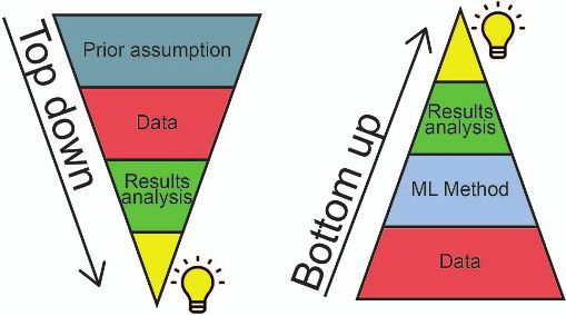
Environ. Res. Lett. 16 (2021) 073008 https://doi.org/10.1088/1748-9326/ac0eb0
TOPICAL REVIEW
Bridging observations, theory and numerical simulation of the
OPEN ACCESS
ocean using machine learning
RECEIVED
23 April 2021 Maike Sonnewald1,2,3,9,∗, Redouane Lguensat4,5, Daniel C Jones6, Peter D Dueben7, Julien Brajard5,8
REVISED
10 June 2021
and V Balaji1,2,4
1
ACCEPTED FOR PUBLICATION Princeton University, Program in Atmospheric and Oceanic Sciences, Princeton, NJ 08540, United States of America
2
25 June 2021 NOAA/OAR Geophysical Fluid Dynamics Laboratory, Ocean and Cryosphere Division, Princeton, NJ 08540, United States of America
3
PUBLISHED University of Washington, School of Oceanography, Seattle, WA, United States of America
4
22 July 2021 Laboratoire des Sciences du Climat et de l’Environnement (LSCE-IPSL), CEA Saclay, Gif Sur Yvette, France
5
LOCEAN-IPSL, Sorbonne Université, Paris, France
6
British Antarctic Survey, NERC, UKRI, Cambridge, United Kingdom
Original Content from 7
this work may be used European Centre for Medium Range Weather Forecasts, Reading, United Kingdom
8
under the terms of the Nansen Center (NERSC), Bergen, Norway
Creative Commons 9
Present address: Princeton University, Program in Atmospheric and Oceanic Sciences, 300 Forrestal Rd., Princeton, NJ 08540,
Attribution 4.0 licence.
United States of America
Any further distribution ∗
Author to whom any correspondence should be addressed.
of this work must
maintain attribution to E-mail: maikes@princeton.edu
the author(s) and the title
of the work, journal Keywords: ocean science, physical oceanography, observations, theory, modelling, supervised machine learning,
citation and DOI. unsupervised machine learning
Abstract
Progress within physical oceanography has been concurrent with the increasing sophistication of
tools available for its study. The incorporation of machine learning (ML) techniques offers exciting
possibilities for advancing the capacity and speed of established methods and for making
substantial and serendipitous discoveries. Beyond vast amounts of complex data ubiquitous in
many modern scientific fields, the study of the ocean poses a combination of unique challenges
that ML can help address. The observational data available is largely spatially sparse, limited to the
surface, and with few time series spanning more than a handful of decades. Important timescales
span seconds to millennia, with strong scale interactions and numerical modelling efforts
complicated by details such as coastlines. This review covers the current scientific insight offered by
applying ML and points to where there is imminent potential. We cover the main three branches of
the field: observations, theory, and numerical modelling. Highlighting both challenges and
opportunities, we discuss both the historical context and salient ML tools. We focus on the use of
ML in situ sampling and satellite observations, and the extent to which ML applications can
advance theoretical oceanographic exploration, as well as aid numerical simulations. Applications
that are also covered include model error and bias correction and current and potential use within
data assimilation. While not without risk, there is great interest in the potential benefits of
oceanographic ML applications; this review caters to this interest within the research community.
1. Introduction have gone hand in hand with the tools available for its
study. Here, the current progress and potential future
1.1. Oceanography: observations, theory, and role of machine learning (ML) techniques is reviewed
numerical simulation and briefly put into historical context. ML adoption is
The physics of the oceans have been of crucial not without risk, but is here put forward as having the
importance, curiosity and interest since prehistoric potential to accelerate scientific insight, performing
times, and today remain an essential element in tasks better and faster, along with allowing avenues of
our understanding of weather and climate, and a serendipitous discovery. This review focuses on phys-
key driver of biogeochemistry and overall marine ical oceanography, but concepts discussed are applic-
resources. The eras of progress within oceanography able across oceanography and beyond.
© 2021 The Author(s). Published by IOP Publishing LtdEnviron. Res. Lett. 16 (2021) 073008 M Sonnewald et al
Perhaps the principal interest in oceanography the era of modern GFD can be seen to stem
was originally that of navigation, for exploration, from linearizing the Navier–Stokes equations, which
commercial and military purposes. Knowledge enabled progress in understanding meteorology and
of the ocean as a dynamical entity with predict- atmospheric circulation. For the ocean, pioneer-
able features—the regularity of its currents and ing dynamicists include Sverdrup, Stommel, and
tides—must have been known for millennia. Know- Munk, whose theoretical work still has relevance
ledge of oceanography likely helped the successful today [182, 232]. As compared to the atmosphere,
colonization of Oceania [180], and similarly Viking the ocean circulation exhibits variability over a much
and Inuit navigation [119], the oldest known dock larger range of timescales, as noted by [183], likely
was constructed in Lothal with knowledge of the spanning thousands of years rather than the few
tides dating back to 2500–1500 BCE [50], and Abu decades of detailed ocean observations available at
Ma’shar of Baghdad in the 8th century CE correctly the time. Yet, there are phenomena at intermediate
attributed the existence of tides to the Moon’s pull. timescales (that is, months to years) which seemed
The ocean measurement era, determining tem- to involve both atmosphere and ocean, e.g. [186],
perature and salinity at depth from ships, starts in and indeed Sverdrup suggests the importance of the
the late 18th century CE. While the tools for a theory coupled atmosphere-ocean system in [234]. In the
of the ocean circulations started to become available 1940s much progress within GFD was also driven by
in the early 19th century CE with the Navier–Stokes the second world war (WWII). The introduction of
equation, observations remained at the core of ocean- accurate navigation through radar introduced with
ographic discovery. The first modern oceanographic WWII worked a revolution for observational oceano-
textbook was published in 1855 by M. Mauri, whose graphy together with bathythermographs intensively
work in oceanography and politics served the slave used for submarine detection. Beyond in situ observa-
trade across the Atlantic, around the same time CO2 ’s tions, the launch of Sputnik, the first artificial satellite,
role in climate was recognized [96, 248]. The first in 1957 heralded the era of ocean observations from
major global observational synthesis of the ocean can satellites. Seasat, launched on the 27th of June 1978,
be traced to the Challenger expeditions of 1873–75 was the first satellite dedicated to ocean observation.
CE [69], where observational data from various areas Oceanography remains a subject that must be
was brought together to gain insight into the global understood with an appreciation of available tools,
ocean. The observational synthesis from the Chal- both observational and theoretical, but also numer-
lenger expeditions gave a first look at the global dis- ical. While numerical GFD can be traced back to
tribution of temperature and salinity including at the early 1900s [2, 31, 209], it became practical
depth, revealing the 3-dimensional structure of the with the advent of numerical computing in the late
ocean. 1940s, complementing that of the elegant deduc-
Quantifying the time mean ocean circulation tion and more heuristic methods that one could
remains challenging, as ocean circulation features call ‘pattern recognition’ that had prevailed before
strong local and instantaneous fluctuations. Improve- [11]. The first ocean general circulation model with
ments in measurement techniques allowed the specified global geometry were developed by Bryan
Swedish oceanographer Ekman to elucidate the and Cox [44, 45] using finite-difference methods.
nature of the wind-driven boundary layer [87]. This work paved the way for what now is a major
Ekman used observations taken on an expedition component of contemporary oceanography. The first
led by the Norwegian oceanographer and explorer coupled ocean-atmosphere model of [167] eventu-
Nansen, where the Fram was intentionally frozen ally led to their use for studies of the coupled Earth
into the Arctic ice. The ‘dynamic method’ was intro- system, including its changing climate. The low-
duced by Swedish oceanographer Sandström and the power integrated circuit that gave rise to computers
Norwegian oceanographer Helland-Hansen [217], in the 1970s also revolutionized observational ocean-
allowing the indirect computation of ocean currents ography, enabling instruments to reliably record
from density estimates under the assumption of a autonomously. This has enabled instruments such as
largely laminar flow. This theory was developed fur- moored current meters and profilers, drifters, and
ther by Norwegian meteorologist Bjerknes into the floats through to hydrographic and velocity profil-
concept of geostrophy, from the Greek geo for earth ing devices that gave rise to microstructure meas-
and strophe for turning. This theory was put to the urements. Of note is the fleet of free-drifting Argo
test in the extensive Meteor expedition in the Atlantic floats, beginning in 2002, which give an extraordin-
from 1925 to 1927 CE; they uncovered a view of the ary global dataset of profiles [212]. Data assimila-
horizontal and vertical ocean structure and circu- tion (DA) is the important branch of modern oceano-
lation that is strikingly similar to our present view graphy combining what is often sparse observational
of the Atlantic meridional overturning circulation data with either numerical or statistical ocean mod-
[177, 210]. els to produce observationally-constrained estim-
While the origins of geophysical fluid dynamics ates with no gaps. Such estimates are referred to as
(GFD) can be traced back to Laplace or Archimedes, an ‘ocean state’, which is especially important for
2Environ. Res. Lett. 16 (2021) 073008 M Sonnewald et al
understanding locations and times with no available gaining insight into the learned mechanisms that
observations. gave rise to ML predictive skill. This is facilitated
Together the innovations within observations, by either building a priori interpretable ML applic-
theory, and numerical models have produced dis- ations or by retrospectively explaining the source
tinctly different pictures of the ocean as a dynam- of predictive skill, coined interpretable and explain-
ical system, revealing it as an intrinsically tur- able artificial intelligence (IAI and XAI, respectively
bulent and topographically influenced circulation [26, 134, 214, 228]). An example of interpretability
[101, 266]. Key large scale features of the circula- could be looking for coherent structures (or ‘clusters’)
tion depend on very small scale phenomena, which within a closed budget where all terms are accounted
for a typical model resolution remain parameterized for. Explainability comes from, for example, tracing
rather than explicitly calculated. For instance, fully the weights within a Neural Network (NN) to determ-
accounting for the subtropical wind-driven gyre cir- ine what input features gave rise to its prediction.
culation and associated western boundary currents With such insights from transparent ML, a syn-
relies on an understanding of the vertical transport thesis between theoretical and observational branches
of vorticity input by the wind and output at the of oceanography could be possible. Traditionally,
sea floor, which is intimately linked to mesoscale theoretical models tend towards oversimplification,
(ca. 100 km) flow interactions with topography [85, while data can be overwhelmingly complicated. For
133]. It has become apparent that localized small- advancement in the fundamental understanding of
scale turbulence (0–100 km) can also impact the ocean physics, ML is ideally placed to identify sali-
larger-scale, time-mean overturning and lateral cir- ent features in the data that are comprehensible to
culation by affecting how the upper ocean interacts the human brain. With this approach, ML could sig-
with the atmosphere [95, 124, 242]. The prominent nificantly facilitate a generalization beyond the limits
role of the small scales on the large scale circula- of data, letting data reveal possible structural errors
tion has important implications for understanding in theory. With such insight, a hierarchy of concep-
the ocean in a climate context, and its representation tual models of ocean structure and circulation could
still hinges on the further development of our fun- be developed, signifying an important advance in our
damental understanding, observational capacity, and understanding of the ocean.
advances in numerical approaches. In this review, we introduce ML concepts
The development of both modern oceanography (section 1.2), and some of its current roles in the
and ML techniques have happened concurrently, as atmospheric and Earth System Sciences (section 1.3),
illustrated in figure 1. This review summarizes the highlighting particular areas of note for ocean applic-
current state of the art in ML applications for phys- ations. The review follows the structure outline illus-
ical oceanography and points towards exciting future trated in figure 2, with the ample overlap noted
avenues. We wish to highlight certain areas where the through cross referencing the text. We review ocean
emerging techniques emanating from the domain of observations (section 2), sparsely observed for much
ML demonstrate potential to be transformative. ML history, but now yielding increasingly clear insight
methods are also being used in closely-related fields into the ocean and its 3D structure. In section 3 we
such as atmospheric science. However, within ocean- examine a potential synergy between ML and the-
ography one is faced with a unique set of challenges ory, with the intent to distil expressions of theoretical
rooted in the lack of long-term and spatially dense understanding by dataset analysis from both numer-
data coverage. While in recent years the surface of the ical and observational efforts. We then progress from
ocean is becoming well observed, there is still a con- theory to models, and the encoding of theory and
siderable problem due to sparse data, particularly in observations in numerical models (section 4). We
the deep ocean. Temporally, the ocean operates on highlight some issues involved with ML-based predic-
timescales from seconds to millennia, and very few tion efforts (section 5), and end with a discussion of
long term time series exist. There is also considerable challenges and opportunities for ML in the ocean sci-
scale-interaction, which also necessitates more com- ences (section 6). These challenges and opportunities
prehensive observations. include the need for transparent ML, ways to support
There remains a healthy scepticism towards some decision makers and a general outlook. Appendix has
ML applications, and calls for ‘trustworthy’ ML are a list of acronyms.
also coming forth from both the European Union and
the United States government (Assessment List for 1.2. Concepts in ML
Trustworthy Artificial Intelligence [ALTAI], and man- Throughout this article, we will mention some
date E.O. 13 960 of 3 December 2020). Within the concepts from the ML literature. We find it then nat-
physical sciences and beyond, trust can be fostered ural to start this paper with a brief introduction to
through transparency. For ML, this means moving some of the main ideas that shaped the field of ML.
beyond the ‘black box’ approach for certain applic- ML, a sub-domain of artificial intelligence (AI),
ations. Moving away from this black box approach is the science of providing mathematical algorithms
and adopting a more transparent approach involves and computational tools to machines, allowing them
3Environ. Res. Lett. 16 (2021) 073008 M Sonnewald et al
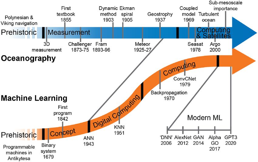
Figure 1. Timeline sketch of oceanography (blue) and ML (orange). The timelines of oceanography and ML are moving towards
each other, and interactions between the fields where ML tool as are incorporated into oceanography has the potential to
accelerate discovery in the future. Distinct ‘events’ marked in grey. Each field has gone through stages (black), with progress that
can be attributed to the available tools. With the advent of computing, the fields were moving closer together in the sense that ML
methods generally are more directly applicable. Modern ML is seeing an very fast increase in innovation, with much potential for
adoption by oceanographers. See table A1 for acronyms.
Figure 2. Machine learning within the components of oceanography. A diagram capturing the general flow of knowledge,
highlighting the components covered in this review. Separating the categories (arrows) is artificial, with ubiquitous feed-backs
between most components, but serves as an illustration.
to perform selected tasks by ‘learning’ from data. the learning process and assess the performance
This field has undergone a series of impressive break- of the ML algorithm. Given a dataset of N pairs
throughs over the last years thanks to the increas- of input-output training examples {(x(i) , y(i) )}i∈1...N
ing availability of data and the recent developments and a loss function L that represents the discrepancy
in computational and data storage capabilities. Sev- between the ML model prediction and the actual out-
eral classes of algorithms are associated with the dif- puts, the parameters θ of the ML model f are found
ferent applications of ML. They can be categorized by solving the following optimization problem:
into three main classes: supervised learning, unsuper-
1 ∑ ( ( (i) ) (i) )
N
vised learning, and reinforcement learning (RL). In
θ ∗ = arg min L f x ;θ ,y . (1)
this review, we focus on the first two classes which θ N
i=1
are the most commonly used to date in the ocean
sciences. If the loss function is differentiable, then gradient
descent based algorithms can be used to solve
equation (1). These methods rely on an iterative tun-
1.2.1. Supervised learning ing of the models’ parameters in the direction of
Supervised learning refers to the task of inferring the negative gradient of the loss function. At each
a relationship between a set of inputs and their iteration k, the parameters are updated as follows:
corresponding outputs. In order to establish this rela-
tionship, a ‘labelled’ dataset is used to constrain θ k+1 = θ k − µ∇L (θ k ) , (2)
4Environ. Res. Lett. 16 (2021) 073008 M Sonnewald et al
where µ is the rate associated with the descent and is interconnected nodes applying geometric trans-
called the learning rate and ∇ the gradient operator. formations (called affine transformations) to
Two important applications of supervised learn- inputs and a nonlinearity function called an ‘activ-
ing are regression and classification. Popular stat- ation function’ [66]
istical techniques such as least squares or ridge
regression, which have been around for a long time, The recent ML revolution, i.e. the so-called deep
are special cases of a popular supervised learning learning (DL) era that began in the early 2010s,
technique called linear regression (in a sense, we may sparked off thanks to the scientific and engineer-
consider a large number of oceanographers to be ing breakthroughs in training neural networks (NN),
early ML practitioners.) For regression problems, we combined with the proliferation of data sources
aim to infer continuous outputs and usually use the and the increasing computational power and stor-
mean squared error (MSE) or the mean absolute error age capacities. The simplest example of this advance-
(MAE) to assess the performance of the regression. ment is the efficient use of the algorithm of back-
In contrast, for supervised classification problems we propagation (known in the geocience community as
sort the inputs to a number of classes or categor- the adjoint method) combined with stochastic gradi-
ies that have been pre-defined. In practice, we often ent descent for the training of multi-layer NNs, i.e.
transform the categories into probability values of NNs with multiple layers, where each layer takes
belonging to some class and use distribution-based the result of the previous layer as an input, applies
distances such as the cross-entropy to evaluate the the mathematical transformations and then yields an
performance of the classification algorithm. input for the next layer [25]. DL research is a field
Numerous types of supervised ML algorithms receiving intense focus and fast progress through its
have been used in the context of ocean research, as use both commercially and scientifically, resulting in
detailed in the following sections. Notable methods new types of ‘architectures’ of NNs, each adapted to
include: particular classes of data (text, images, time series,
etc) [155, 219]. We briefly introduce the most pop-
ular architectures used in deep learning research and
• Linear univariate (or multivariate) regression (LR), highlight some applications:
where the output is a linear combination of some
explanatory input variables. LR is one of the first • Multilayer perceptrons (MLP): when used without
ML algorithms to be studied extensively and used qualification, this term refers to fully connected
for its ease of optimization and its simple statistical feed forward multilayered neural networks. They
properties [181]. are composed of an input layer that takes the
• k-nearest neighbours (KNN), where we consider an input data, multiple hidden layers that convey the
input vector, find its k closest points with regard to information in a ‘feed forward’ way (i.e. from input
a specified metric, then classify it by a plurality vote to output with no exchange backwards), and finally
of these k points. For regression, we usually take the an output layer that yields the predictions. Any
average of the values of the k neighbours. KNN is neuron in a MLP is connected to all the neurons
also known as ‘analog methods’ in the numerical in the previous and to those of next layer, thus the
weather prediction community [163]. use of the term ‘fully connected’. MLPs are mostly
• Support vector machines (SVM) [61], where the used for tabular data.
classification is done by finding a linear separating • Convolutional neural networks (ConvNet): con-
hyperplane with the maximal margin between two trarily to MLPs, ConvNets are designed to take
classes (the term ‘margin’ here denotes the space into account the local structure of particular type
between the hyperplane and the nearest points in of data such as text in 1D, images in 2D, volu-
either class.) In case of data which cannot be separ- metric images in 3D, and also hyperspectral data
ated linearly, the use of the kernel trick projects the such as that used in remote sensing. Inspired by
data into a higher dimension where the linear sep- the animal visual cortex, neurons in ConvNets are
aration can be done. Support vector regression (SVR) not fully connected, instead they receive informa-
are an adaption of SVMs for regression problems. tion from a subarea spanned by the previous layer
• Random forests (RF) that are a composition of a called the ‘receptive field’. In general, a ConvNet is
multitude of decision trees (DT). DTs are construc- a feed forward architecture composed of a series of
ted as a tree-like composition of simple decision convolutional layers and pooling layers and might
rules [29]. also be combined with MLPs. A convolution is
• Gaussian process regression (GPR) [264], also called the application of a filter to an input that res-
kriging, is a general form of the optimal interpola- ults in an activation. One convolutional layer con-
tion algorithm, which has been used in the ocean- sist of a group of ‘filters’ that perform mathemat-
ographic community for a number of years ical discrete convolution operations, the result of
• Neural networks (NN), a powerful class of universal these convolutions are called ‘feature maps’. The
approximators that are based on compositions of filters along with biases are the parameters of the
5Environ. Res. Lett. 16 (2021) 073008 M Sonnewald et al
ConvNet that are learned through backpropaga- as a generalization of the k-means algorithm that
tion and stochastic gradient descent. Pooling lay- assumes the data can be represented by a mixture
ers serve to reduce the resolution of feature maps (i.e. linear combination) of a number of multi-
which lead to compressing the information and dimensional Gaussian distributions [176].
speeding up the training of the ConvNet, they • Kohonen maps [also called Self Organizing Maps
also help the ConvNet become invariant to small (SOM)] is a NN based clustering algorithm that
shift in input images [155]. ConvNets benefited leverages topology of the data; nearby locations in
much from the advancements in GPU computing a learned map are placed in the same class [147]. K-
and showed great success in the computer vision means can be seen as a special case of SOM with no
community. information about the neighbourhood of clusters.
• Recurrent neural networks (RNN): with an aim • t-SNE and UMAP are two other clustering
to model sequential data such as temporal signals algorithms which are often used for not only find-
or text data, RNNs were developed with a hidden ing clusters but also because of their data visu-
state that stores information about the history of alization properties which enables a two or three
the sequences presented to its inputs. While the- dimensional graphical rendition of the data [175,
oretically attractive, RNNs were practically found 250]. These methods are useful for representing the
to be hard to train due to the exploding/vanish- structure of a high-dimensional dataset in a small
ing gradient problems, i.e. backpropagated gradi- number of dimensions that can be plotted. For
ents tend to either increase too much or shrink the projection, they use a measure of the ‘distance’
too much at each time step [127]. Long short term or ‘metric’ between points, which is a sub-field
memory (LSTM) architecture provided a solution of mathematics where methods are increasingly
to this problem through the use of special hid- implemented for t-SNE or UMAP.
den units [219]. LSTMs are to date the most pop- • Principal Component Analysis (PCA) [191], the
ular RNN architectures and are used in several simplest and most popular dimensionality reduc-
applications such as translation, text generation, tion algorithm. Another term for PCA is Empir-
time series forecasting, etc. Note that a variant ical Orthogonal Function analysis (EOF), which
for spatiotemporal data was developed to integ- has been used by physical oceanographers for many
rate the use of convolutional layers, this is called years, also called Proper Orthogonal Decomposi-
ConvLSTM [224]. tion (POD) in computational fluids literature.
• Autoencoders (AE) are NN-based dimensionality
1.2.2. Unsupervised learning reduction algorithms, consisting of a bottleneck-
Unsupervised learning is another major class of ML. like architecture that learns to reconstruct the input
In these applications, the datasets are typically unla- by minimizing the error between the output and
belled. The goal is then to discover patterns in the the input (i.e. ideally the data given as input and
data that can be used to solve particular problems. output of the autoencoder should be interchange-
One way to say this is that unsupervised classification able). A central layer with a lower dimension than
algorithms identify sub-populations in data distribu- the original inputs’ dimension is called a ‘code’
tions, allowing users to identify structures and poten- and represents a compressed representation of the
tial relationships among a set of inputs (which are input [149].
sometimes called ‘features’ in ML language). Unsu- • Generative modelling: a powerful paradigm that
pervised learning is somewhat closer to what humans learns the latent features and distributions of a
expect from an intelligent algorithm, as it aims to dataset and then proceeds to generate new samples
identify latent representations in the structure of the that are plausible enough to belong to the ini-
data while filtering out unstructured noise. At the tial dataset. Variational auto-encoders (VAEs) and
NeurIPS 2016 conference, Yann LeCun, a DL pion- generative adversarial networks (GANS) are two
eer researcher, highlighted the importance of unsu- popular techniques of generative modelling that
pervised learning using his cake analogy: ‘If machine benefited much from the DL revolution [111, 144].
learning is a cake, then unsupervised learning is the
actual cake, supervised learning is the icing, and RL is Between supervised and unsupervised learning
the cherry on the top.’ lies semi-supervised learning. It is a special case where
Unsupervised learning is achieving considerable one has access to both labelled and unlabelled data. A
success in both clustering and dimensionality reduc- classical example is when labelling is expensive, lead-
tion applications. Some of the unsupervised tech- ing to a small percentage of labelled data and a high
niques that are mentioned throughout this review are: percentage of unlabelled data.
Reinforcement learning is the third paradigm of
• k-means, a popular and simple space-partitioning ML; it is based on the idea of creating algorithms
clustering algorithm that finds classes in a dataset where an agent explores an environment with the
by minimizing within-cluster variances [230]. aim of reaching some goal. The agent learns through
Gaussian Mixture Models (GMMs) can be seen a trial and error mechanism, where it performs an
6Environ. Res. Lett. 16 (2021) 073008 M Sonnewald et al
action and receives a response (reward or punish- out a vast computation by hand across all available
ment), the agent learns by maximizing the expec- data. This led to the discovery of the Southern Oscil-
ted sum of rewards [238]. The DL revolution did lation, the seesaw in the West-East temperature gradi-
also affect this field and led to the creation of a new ent in the Pacific, which we know now by its modern
field called deep reinforcement learning (Deep RL) name, El Niño Southern Oscillation (ENSO). Bey-
[233]. A popular example of Deep RL that got huge ond observed correlations, theories of ENSO and its
media attention is the algorithm AlphaGo developed emergence from coupled atmosphere-ocean dynam-
by DeepMind which beat human champions in the ics appeared decades later [270]. Walker speaks of
game of Go [225]. statistical methods of discovering ‘weather connec-
The importance of understanding why an ML tions in distant parts of the earth’, or teleconnections.
method arrived at a result is not confined to ocean- The ENSO-monsoon teleconnection remains a key
ographic applications. Unsupervised ML lends itself element in diagnosis and prediction of the Indian
more readily to being interpreted (IAI), but for monsoon [236, 237]. These and other data-driven
example for methods building on DL or NN in gen- methods of the pre-ML era are surveyed in [42]. ML-
eral, a growing family of methods collectively referred based predictive methods targeted at ENSO are also
to as additive feature attribution (AFA) is becom- being established [120]. Here, the learning is not dir-
ing popular, largely applied for XAI. AFA methods ectly from observations but from models and reana-
aim to explain predictive skill retrospectively. These lysis data, and outperform some dynamical models in
methods include connection weight approaches, local forecasting ENSO.
interpretable model-agnostic explanations (LIME), There is an interplay between data-driven meth-
Shapley additive explanation (SHAP) and layer-wise ods and physics-driven methods that both strive to
relevance propagation (LRP) [26, 153, 165, 179, 193, create insight into many complex systems, where
208, 228, 246]. Non-AFA methods rooted in ‘saliency’ the ocean and the wider Earth system science are
mapping also exist [174]. examples. As an example of physics-driven meth-
The goal of this review paper is not to delve into ods [11], Bjerknes and other pioneers discussed in
the definitions of ML techniques but only to briefly section 1.1 formulated accurate theories of the general
introduce them to the reader and recommend ref- circulation that were put into practice for forecast-
erences for further investigation. The textbook by ing with the advent of digital computing. Advances in
Bishop [30] covers essentials of the fields of pattern numerical methods led to the first practical physics-
recognition and Hsieh’s book [131] is probably one of based atmospheric forecast [199]. Until that time,
earliest attempts at writing a comprehensive review of forecasting often used data-driven methods ‘that were
ML methods targeted at earth scientists. Another not- neither algorithmic nor based on the laws of phys-
able review of statistical methods for physical ocean- ics’ [187]. ML offers avenues to a synthesis of data-
ography is the paper by Wikle et al [262]. We also driven and physics-driven methods. In recent years,
refer the interested reader to the book of Goodfellow as outlined below in section 4.3, new processors and
et al [25] to learn more about the theoretical found- architectures within computing have allowed much
ations of DL and some of its applications in science progress within forecasting and numerical modelling
and engineering. overall. ML methods are poised to allow Earth sys-
tem science modellers to increase the efficient use of
1.3. ML in atmospheric and the wider earth system modern hardware even further. It should be noted
sciences however that ‘classical’ methods of forecasting such
Precursors to modern ML methods, such as regres- as analogues also have become more computationally
sion and principal component analysis, have of course feasible, and demonstrate equivalent skill, e.g. [73].
been used in many fields of Earth system science for The search for analogues has become more computa-
decades. The use of PCA, for example, was popular- tionally tractable as well, although there may also be
ized in meteorology in [162], as a method of dimen- limits here [76].
sionality reduction of large geospatial datasets, where Advances in numerical modelling brought in
Lorenz also speculates here on the possibility of purely additional understanding of elements in Earth sys-
statistical methods of long-term weather prediction tem science which are difficult to derive, or represent
based on a representation of data using PCA. Meth- from first principles. Examples include cloud micro-
ods for discovering correlations and links, including physics or interactions with the land surface and bio-
possible causal links, between dataset features using sphere. For capturing cloud processes within mod-
formal methods have seen much use in Earth sys- els, the actual processes governing clouds take place
tem science. e.g. [18]. For example, Walker [256] was at scales too fine to model and will remain out of
tasked with discovering the cause for the interannual reach of computing for the foreseeable future [221].
fluctuation of the Indian monsoon, whose failure A practical solution to this is finding a representation
meant widespread drought in India, and in colonial of the aggregate behaviour of clouds at the resolution
times also famine [68]. To find possible correlations, of a model grid cell. This has proved quite difficult
Walker put to work an army of Indian clerks to carry and progress over many decades has been halting
7Environ. Res. Lett. 16 (2021) 073008 M Sonnewald et al
[36]. The use of ML in deriving representations example of such methods. While ESD emphasized the
of clouds is now an entire field of its own. Early downscaling aspect, all of these downscaling meth-
results include the results of [105], using NNs to ods include a substantial element of bias correction.
emulate a ‘super-parameterized’ model. In the super- This is highlighted in the name of some of the pop-
parameterized model, there is a clear (albeit artifi- ular methods such as Bias Correction and Spatial
cial) separation of scales between the ‘cloud scale’ Downscaling [265] and Bias Corrected Constructed
and the large scale flow. When this scale separation Analogue [171]. These are trend-preserving statistical
assumption is relaxed, some of the stability problems downscaling algorithms, that combine bias correction
associated with ML re-emerge [41]. There is also a with the analogue method of Lorenz [164]. ML meth-
fundamental issue of whether learned relationships ods are rapidly coming to dominate the field as dis-
respect basic physical constraints, such as conserva- cussed in section 5.1, with examples ranging from
tion laws [160]. Recent advances [27, 268] focus on precipitation (e.g. [252]), surface winds and solar
formulating the problem in a basis where invariances outputs [231], as well as to unresolved river trans-
are automatically maintained. But this still remains port [108]. Downscaling methods continue to make
a challenge in cases where the physics is not fully the assumption that transfer functions learned from
understood. present-day climate continue to hold in the future.
There are at least two major efforts for the sys- This stationarity assumption is a potential weakness
tematic use of ML methods to constrain the cloud of data-driven methods [74, 192], that requires a syn-
model representations in GCMs. First, the calibrate- thesis of data-driven and physics-based methods as
emulate-sample (CES [58, 81]) approach uses a more well.
conventional model for a broad calibration of para-
meters also referred to as ‘tuning’[129]. This is fol- 2. Ocean observations
lowed by an emulator, that calibrates further and
quantifies uncertainties. The emulator is an ML- Observations continue to be key to oceanographic
based model that reproduces most of the variabil- progress, with ML increasingly being recognized as
ity of the reference model, but at a lower computa- a tool that can enable and enhance what can be
tional cost. The low computational cost enables the learned from observational data, performing conven-
emulator to be used to produce a large ensemble tional tasks better/faster, as well as bring together dif-
of simulations, that would have been too computa- ferent forms of observations, facilitating comparison
tionally expensive to produce using the model that with model results. ML offers many exciting oppor-
the emulator is based on. It is important to retain tunities for use with observations, some of which are
the uncertainty quantification aspect (represented by covered in this section and in section 5 as supporting
the emulated ensemble) in the ML context, as it is predictions and decision support.
likely that the data in a chaotic system only imper- The onset of the satellite observation era brought
fectly constrain the loss function. Second, emulat- with it the availability of a large volume of effect-
ors can be used to eliminate implausible paramet- ively global data, challenging the research community
ers from a calibration process, demonstrated by the to use and analyse this unprecedented data stream.
HighTune project [63, 130]. This process can also Applications of ML intended to develop more accur-
identify ‘structural error’, indicating that the model ate satellite-driven products go back to the 90s [241].
formulation itself is incorrect, when no parameter These early developments were driven by the data
choices can yield a plausible solution. Model errors availability, distributed in normative format by the
are discussed in section 5.1. In an ocean context, the space agencies, and also by the fact that models
methods discussed here can be a challenge due to describing the data were either empirical (e.g. mar-
the necessary forwards model component. Note also, ine biogeochemistry [218]) or too computationally
that ML algorithms such as GPR are ubiquitous in costly and complex (e.g. radiative transfer [143]).
emulating problems thanks to their built-in uncer- More recently, ML algorithms have been used to
tainty quantification. GPR methods are also popular fuse several satellite products [116] and also satel-
because their application involves a low number of lite and in-situ data [52, 70, 142, 170, 185]. For the
training samples, and function as inexpensive substi- processing of satellite data, ML has proven to be a
tutes for a forward model. valuable tool for extracting geophysical information
Model resolution that is inadequate for many from remotely sensed data (e.g. [51, 82]), whereas
practical purposes has led to the development of data- a risk of using only conventional tools is to exploit
driven methods of ‘downscaling’. For example climate only a more limited subset of the mass of data avail-
change adaptation decision-making at the local level able. These applications are based mostly on instant-
based on climate simulations too coarse to feature aneous or very short-term relationships and do not
enough detail. Most often, a coarse-resolution model address the problem of how these products can be
output is mapped onto a high-resolution reference used to improve our ability to understand and fore-
truth, for example given by observations [4, 251]. cast the oceanic system. Further use for current recon-
Empirical-statistical downscaling (ESD, [24]) is an struction using ML [169], heat fluxes [106], the
8Environ. Res. Lett. 16 (2021) 073008 M Sonnewald et al
3-dimensional circulation [228], and ocean heat con- used, yielding products used in operational contexts.
tent [135] are also being explored. For example, Kriging is a popular technique that
There is also an increasingly rich body of literat- was successfully applied to altimetry [154], as it can
ure mining ocean in-situ observations. These lever- account for observation from multiple satellites with
age a range of data, including Argo data, to study a different spatio-temporal sampling. In its simplest
range of ocean phenomena. Examples include assess- form, kriging estimates the value of an unobserved
ing North Atlantic mixed layers [172], describing spa- location as the linear combination of available obser-
tial variability in the Southern Ocean [138], detecting vations. Kriging also yields the uncertainty of this
El Niño events [128], assessing how North Atlantic estimate, which has made it popular in geostatistics.
circulation shifts impacting heat content [71], and EOF-based techniques are also attracting increasing
finding mixing hot spots [213]. ML has also been attention with the proliferation of data. For example,
successfully applied to ocean biogeochemistry. While the DINEOF algorithm [6] leverages the availabil-
not covered in detail here, examples include mapping ity of historical datasets, to fill in spatial gaps within
oxygen [110] and CO2 fluxes [46, 152, 259]. new observations. This is done via projection onto
Modern in-situ classification efforts are often the space spanned by dominant EOFs of the historical
property-driven, carrying on long traditions within data. The use of advanced supervised learning, such
physical oceanography. For example, characteristic as DL, for this problem in an oceanographic contexts
groups or ‘clusters’ of salinity, temperature, density or is still in its infancy. Attempts exist in the literature,
potential vorticity have typically been used to delin- including deriving a DL equivalent of DINEOF for
eate important water masses and to assess their spatial interpolating SST [19].
extent, movement, and mixing [121, 126]. However,
conventional identification/classification techniques 3. Exchanges between observations and
assume that these properties stay fixed over time. The theory
techniques largely do not take interannual and longer
timescale variability into account. The prescribed Progress within observations, modelling, and theory
ranges used to define water masses are often some- go hand in hand, and ML offers a novel method for
what ad-hoc and specific (e.g. mode waters are often bridging the gaps between the branches of ocean-
tied to very restrictive density ranges) and do not gen- ography. When describing the ocean, theoretical
eralize well between basins or across longer timescales descriptions of circulation tend to be oversimplified,
[9]. Although conventional identification/classifica- but interpreting basic physics from numerical sim-
tion techniques will continue to be useful well into ulations or observations alone is prohibitively diffi-
the future, unsupervised ML offers a robust, alternat- cult. Progress in theoretical work has often come from
ive approach for objectively identifying structures in the discovery or inference of regions where terms in
oceanographic observations [33, 138, 197, 213]. an equation may be negligible, allowing theoretical
To analyse data, dimensionality and noise reduc- developments to be focused with the hope of obser-
tion methods have a long history within oceano- vational verification. Indeed, progress in identifying
graphy. PCA is one such method, which has had a negligible terms in fluid dynamics could be said to
profound influence on oceanography since Lorenz underpin GFD as a whole [249]. For example, Sver-
first introduced it to the geosciences in 1956 [162]. drup’s theory [235] of ocean regions where the wind
Despite the method’s shortcomings related to strong stress curl is balanced by the Coriolis term inspired a
statistical assumptions and misleading applications, search for a predicted ‘level of no motion’ within the
it remains a popular approach [178]. PCA can be ocean interior.
seen as a super sparse rendition of k-means cluster- The conceptual and numerical models that
ing [72] with the assumption of an underlying nor- underlie modern oceanography would be less valu-
mal distribution in its commonly used form. Overall, able if not backed by observational evidence, and
different forms of ML can offer excellent advantages similarly, findings in data from both observations
over more commonly used techniques. For example, and numerical models can reshape theoretical mod-
many clustering algorithms can be used to reduce els [101]. ML algorithms are becoming heavily used
dimensionality according to how many significant to determine patterns and structures in the increas-
clusters are identifiable in the data. In fact, unsuper- ing volumes of observational and modelled data [33,
vised ML can sidestep statistical assumptions entirely, 47, 71, 128, 138, 139, 172, 197, 213, 229, 240]. For
for example by employing density-based methods example, ML is poised to help the research com-
such as DBSCAN [227]. Advances within ML are munity reframe the concept of ocean fronts in ways
making it increasingly possible and convenient to that are tailored to specific domains instead of ways
take advantage of methods such as t-SNE [227] and that are tied to somewhat ad-hoc and overgeneralized
UMAP, where the original topology of the data can property definitions [54]. Broadly speaking, this area
be conserved in a low-dimensional rendition. of work largely utilizes unsupervised ML and is thus
Interpolation of missing data in oceanic fields is well-positioned to discover underlying structures
another application where ML techniques have been and patterns in data that can help identify negligible
9Environ. Res. Lett. 16 (2021) 073008 M Sonnewald et al
achieved using conventional methods but is signi-
ficantly facilitated by ML, as modern data in its
often complicated, high dimensional, and volumin-
ous form complicates objective analysis. ML, through
its ability to let structures within data emerge, allows
the structures to be systematically analysed. Such
structures can emerge as regions of coherent covari-
ance (e.g. using clustering algorithms from unsuper-
Figure 3. Cartoon of the role of data within vised ML), even in the presence of highly non-linear
oceanography. While eliminating prior assumptions and intricate covariance [227]. Such structures can
within data analysis is not possible, or even desirable, then be investigated in their own right and may
ML applications can enhance the ability to perform
pure data exploration. The ‘top down’ approach (left) potentially form the basis of new theories. Such
refers to a more traditional approach where the exploration is facilitated by using an ML approach
exploration of the data is firmly grounded in prior
knowledge and assumptions. Using ML, how data is in combination with IAI and XAI methods as appro-
used in oceanographic research and beyond can be priate. Unsupervised ML lends itself more readily
changed by taking a ‘bottom up’ data-exploration to IAI and to many works discussed above. Object-
centred approach, allowing the possibility for
serendipitous discovery. ive analysis that can be understood as IAI can also
be applied to explore theoretical branches of ocean-
ography, revealing novel structures [47, 229, 240].
Examples where ML and theoretical exploration have
terms or improve a conceptual model that was previ- been used in synergy by allowing interpretability,
ously empirical. In this sense, ML methods are well- explainability, or both within oceanography include
placed to help guide and reshape established theor- [228, 269], and the concepts are discussed further in
etical treatments, for example by highlighting over- section 6.
looked features. A historical analogy can be drawn As an increasingly operational endeavour, phys-
to d’Alembert’s paradox from 1752 (or the hydro- ical oceanography faces pressures apart from fun-
dynamic paradox), where the drag force is zero on damental understanding due to the increasing
a body moving with constant velocity relative to the complexity associated with enhanced resolution or
fluid. Observations demonstrated that there should the complicated nature of data from both observa-
be a drag force, but the paradox remained unsolved tions and numerical models. For advancement in the
until Prandtl’s 1904 discovery of a thin boundary fundamental understanding of ocean physics, ML
layer that remained as a result of viscous forces. Dis- is ideally placed to break this data down to let sali-
coveries like Prandtl’s can be difficult, for example ent features emerge that are comprehensible to the
because the importance of small distinctions that human brain.
here form the boundary layer regime can be over-
looked. ML has the ability to be both objective, and 3.1. ML and hierarchical statistical modelling
also to highlight key distinctions like a boundary The concept of a model hierarchy is described by
layer regime. ML is ideally poised to make discover- [125] as a way to fill the ‘gap between simulation
ies possible through its ability to objectively analyse and understanding’ of the Earth system. A hier-
the increasingly large and complicated data available. archy consists of a set of models spanning a range
Using conventional analysis tools, finding patterns of complexities. One can potentially gain insights
inadvertently rely on subjective ‘standards’ e.g. how by examining how the system changes when mov-
the depth of the mixed layer or a Southern Ocean ing between levels of the hierarchy, i.e. when vari-
front is defined [54, 75, 243]. Such standards leave ous sources of complexity are added or subtracted,
room for bias and confusion, potentially perpetu- such as new physical processes, smaller-scale features,
ating unhelpful narratives such as those leading to or degrees of freedom in a statistical description.
d’Alembert’s paradox. The hierarchical approach can help sharpen hypo-
With an exploration of a dataset that moves bey- theses about the oceanographic system and inspire
ond preconceived notions comes the potential for new insights. While perhaps conceptually simple, the
making entirely new discoveries. It can been argued practical application of a model hierarchy is non-
that much of the progress within physical oceano- trivial, usually requiring expert judgement and cre-
graphy has been rooted in generalizations of ideas put ativity. ML may provide some guidance here, for
forward over 30 years ago [101, 137, 184]. This found- example by drawing attention to latent structures
ation can be tested using data to gain insight in a in the data. In this review, we distinguish between
‘top-down’ manner (figure 3). ML presents a possible statistical and numerical ML models used for this
opportunity for serendipitous discovery outside of purpose. For ML-mediated models, a goal could
this framework, effectively using data as the founda- be discovering other levels in the model hierarchy
tion and achieving insight purely through its objective from complex models [11]. The models discussed in
analysis in a ‘bottom up’ fashion. This can also be sections 2 and 3 constitute largely statistical models,
10Environ. Res. Lett. 16 (2021) 073008 M Sonnewald et al
such as ones constructed using a k-means applica- is a well-understood approximate boundary between
tion, GANs, or otherwise. This section discusses the polar and subtropical waters. By contrast, more com-
concept of hierarchical models in a statistical sense, plex models capture more structure but are harder to
and section 4.2 explores the concept of numerical interpret using our current conceptual understand-
hierarchical models. A hierarchical statistical model ing of ocean structure and dynamics [138]. In this
can be described as a series of model descriptions way, a collection of statistical models with different
of the same system from very low complexity (e.g. a values of K constitutes a model hierarchy, in which
simple linear regression) to arbitrarily high. In theory, one builds understanding by observing how the rep-
any statistical model constructed with any data from resentation of the system changes when sources of
the ocean could constitute a part of this hierarchy, but complexity are added or subtracted [125]. Note that
here we restrict our discussion to models constructed for the example of k-means, while a range of K val-
from the same or very similar data. ues may be reasonable, this does not largely refer to
The concept of exploring a hierarchy of models, merely adjusting the value of K and re-interpreting
either statistical or otherwise, using data could also the result. This is because, for example, if one moves
be expressed as searching for an underlying manifold from K = 2 to K = 3 using k-means, there is no a pri-
[161]. The notion of identifying the ‘slow manifold’ ori reason to assume they would both give physically
postulates that the noisy landscape of a loss function meaningful results. What is meant instead is similar
for one level of the hierarchy, conceals a smoother to the type of hierarchical clustering that is able to
landscape in another level. As such, it should be plaus- identify different sub-groups and organize them into
ible to identify a continuum of system descriptions. larger overarching groups according to how similar
ML has the potential to assist in revealing such an they are to one another. This is a distinct approach
underlying slow manifold, as described above. For within ML that relies on the ability to measure a ‘dis-
example, equation discovery methods shown prom- tance’ between data points. This rationale reinforces
ise as they aim to find closed form solutions to the view that ML can be used to build our concep-
the relations within datasets representing terms in a tual understanding of physical systems, and does not
parsimonious representation (e.g. [100, 220, 269] are need to be used simply as a ‘black box’. It is worth
examples in line with [11]). Similarly, unsupervised noting that the axiom that is being relied on here is
equation exploration could hold promise for utilizing that there exists an underlying system that the ML
formal ideas of hypothesis forming and testing within application can approximate using the available data.
equation space [140]. With incomplete and messy data, the tools available
In oceanographic ML applications, there are tun- to assess the fit of a statistical model only provide
able parameters that are often only weakly con- an estimate of how wrong it is certain to be. To cre-
strained. A particular example is the total number ate a statistically rigorous hierarchy, not only does
of classes K in unsupervised classification problems the overall co-variance structure/topology need to be
[138, 139, 172, 227, 229]. Although one can estim- approximated, but also the finer structures that would
ate the optimal value K ∗ for the statistical model, be found within these overarching structures. If this
for example by using metrics that reward increased identification process is successful, then the structures
likelihood and penalize overfitting (e.g. the Bayesian can be grouped with accuracy as defined by statist-
information criteria (BIC) or the Akaike informa- ical significance. This can pose a formidable challenge
tion criterion (AIC)), in practice it is rare to find that ML in isolation cannot address; it requires guid-
a clear value of K ∗ in oceanographic applications. ance from domain experts. For example, within ocean
Often, tests like BIC or AIC return either a range ecology, [227] derived a hierarchical model by group-
of possible K ∗ values, or they only indicate a lower ing identified clusters according to ecological simil-
bound for K. This is perhaps because oceanographic arity. In physical oceanography, [213] grouped some
data is highly correlated across many different spa- identified classes together into zones using established
tial and temporal scales, making the task of separating oceanographic knowledge, in a step from a more
the data into clear sub-populations a challenging one. complex statistical model to a more simplified one
That being said, the parameter K can also be inter- that is easier to interpret. When performing such
preted as the complexity of the statistical model. A groupings, one has to pay attention to a balance of
model with a smaller value of K will potentially be statistical rigour and domain knowledge. Discover-
easier to interpret because it only captures the domin- ing rigorous and useful hierarchical models should
ant sub-populations in the data distribution. In con- hypothetically be possible, as demonstrated by the
trast, a model with a larger value of K will likely be self-similarity found in many natural systems includ-
harder to interpret because it captures more subtle ing fluids, but limited and imperfect data greatly
features in the data distribution. For example, when complicate the search, meaning that checking for stat-
applied to Southern Ocean temperature profile data, istical rigour is important.
a simple two-class profile classification model will As a possible future direction, assessing models
tend to separate the profiles into those north and using IAI and XAI and known physical relationships
south of the Antarctic Circumpolar Current, which will likely make finding hierarchical models that are
11You can also read