Polygon Laplacian Made Simple - Computer Graphics ...
←
→
Page content transcription
If your browser does not render page correctly, please read the page content below
EUROGRAPHICS 2020 / U. Assarsson and D. Panozzo                                                                                           Volume 39 (2020), Number 2
(Guest Editors)

                                                 Polygon Laplacian Made Simple

                                           Astrid Bunge1†              Philipp Herholz2 †     Misha Kazhdan3         Mario Botsch1

                                  1 Bielefeld   University, Germany          2 ETH   Zurich, Switzerland   3 Johns   Hopkins University, USA

        Abstract

        The discrete Laplace-Beltrami operator for surface meshes is a fundamental building block for many (if not most) geometry pro-
        cessing algorithms. While Laplacians on triangle meshes have been researched intensively, yielding the cotangent discretization
        as the de-facto standard, the case of general polygon meshes has received much less attention. We present a discretization of
        the Laplace operator which is consistent with its expression as the composition of divergence and gradient operators, and is
        applicable to general polygon meshes, including meshes with non-convex, and even non-planar, faces. By virtually inserting
        a carefully placed point we implicitly refine each polygon into a triangle fan, but then hide the refinement within the matrix
        assembly. The resulting operator generalizes the cotangent Laplacian, inherits its advantages, and is empirically shown to be
        on par or even better than the recent polygon Laplacian of Alexa and Wardetzky [AW11] — while being simpler to compute.
        CCS Concepts
        • Computing methodologies → Mesh geometry models; • Theory of computation → Computational geometry;

1. Introduction                                                                                  In this paper we propose a surprisingly simple, yet very effective
                                                                                              discretization of the polygon Laplace operator. Inserting a carefully
The Laplace-Beltrami operator, or Laplacian for short, plays a
                                                                                              placed vertex for every polygon allows us to define a refined trian-
prominent role in geometric modeling and related fields. As a gen-
                                                                                              gulation that retains the symmetries and defines a sensible surface
eralization of the second derivative to functions defined on surfaces
                                                                                              consistent with the polygon mesh. Using the Galerkin method, we
it is intimately related to the notion of curvature and signal frequen-
                                                                                              then coarsen the cotangent Laplacian defined over the triangulation
cies. With triangle meshes being the standard surface representation
                                                                                              to obtain a Laplacian on the original polygon mesh, completely hid-
in computer graphics and geometry processing, the discretization
                                                                                              ing the auxiliary points from the user by encapsulating them within
of the Laplace operator for triangular elements has received a lot
                                                                                              the matrix assembly stage.
of attention over the years, with the classical cotangent discretiza-
tion [Mac49, Dzi88, PP93, DMSB99] being the de-facto standard.                                   Our discrete Laplacian operator acts directly on functions de-
                                                                                              fined on the vertices of a general polygon mesh. It works accu-
   Discrete Laplacians for polygon meshes have been much less
                                                                                              rately and robustly even in the presence of non-planar and non-
well investigated, even though polygon meshes, in particular quad
                                                                                              convex faces. By leveraging the cotangent Laplacian in the core
meshes, are ubiquitous in modern production pipelines (and higher-
                                                                                              of our discretization, we inherit all its benefits. The absence of
order polygons are considered more noble in the 1884 novel Flat-
                                                                                              tweakable parameters makes our operator intuitive and easy to
land [Abb84]). A straightforward approach would be to triangulate
                                                                                              use in practice. Even though our method is quite simple and easy
all polygons and apply the well-defined triangle-based operators.
                                                                                              to implement, we will make our source code freely available at
Unfortunately this approach does not work well in many cases.
                                                                                              https://github.com/mbotsch/polygon-laplacian.
Polygon meshes are commonly designed to align to certain surface
features and capture symmetries of the shape. Introducing an arbi-
trary triangulation can break these properties and lead to noticeable                         2. Related Work
artifacts. Alexa and Wardetzky [AW11] proposed a discrete Lapla-
cian that directly operates on two-manifold polygon meshes and                                Laplacians for triangle meshes The main goal when construct-
avoids these problems. However, their operator relies on a suitable                           ing a discrete Laplacian is to retain as many properties from the
choice of parameter, which can considerably influence the results                             smooth setting as possible. While the classical cotangent Laplace
and might not be easy to find, as we show in Section 5.                                       operator [Mac49] is negative semi-definite, symmetric, and has
                                                                                              linear precision—meaning that the operator yields zero for linear
                                                                                              functions defined over a planar domain—it fails to maintain the
† the first two authors contributed equally                                                   maximum principle. As a consequence, parametrizations obtained

 c 2020 The Author(s)
Computer Graphics Forum c 2020 The Eurographics Association and John
Wiley & Sons Ltd. Published by John Wiley & Sons Ltd.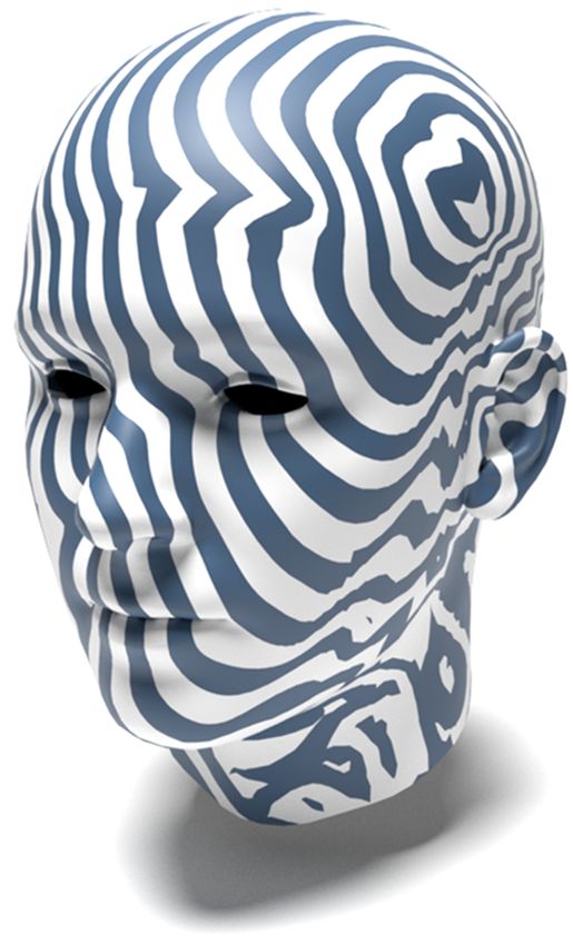
A. Bunge, P. Herholz, M. Kazhdan, M. Botsch / Polygon Laplacian Made Simple
with this discretization can suffer from flipped triangles. In con- 3. Math Review
trast, the combinatorial Laplacian [Tau95, Zha04] guarantees the
Our approach for defining a polygon Laplacian proceeds in two
maximum principle while failing to have linear precision. Bobenko
steps. First, we refine the polygon mesh to define a triangle mesh
and Springborn [BS07] introduced a discrete Laplacian based on
on which the standard cotangent Laplacian is defined. Then, to ob-
the intrinsic Delaunay triangulation. While guaranteeing the max-
tain a Laplacian on the initial polygon mesh, we use the Galerkin
imum principle, this operator is defined over an intrinsic mesh
method to coarsen the cotangent Laplacian. In the following we
with different connectivity. Recently, an efficient data structure for
briefly review both the derivation of Laplacians on triangle meshes
the representation of these meshes has been introduced [SSC19].
[BKP∗ 10] and the Galerkin method [Fle84].
The idea of intrinsic triangulations does not extend to the case
of non-planar polygon meshes due to the lack of a well defined
surface. Other discretizations include the Laplacian of Belkin et Laplacians on triangle meshes
al. [BSW08] that provides point-wise convergence and the octree-
Consider a triangle mesh M = (V, T ) with vertices V and triangles
based Laplacian [CLB∗ 09] defined to support multigrid solvers. In
T . Let |V | and |T | be the numbers of vertices and triangles, respec-
general, Wardetzky et al. [WMKG07] have shown that there cannot
tively, and let {φ1 , . . . , φ|V | } be the hat basis (with φi the piecewise
exist a discretization that fulfills a certain set of properties for all
linear function that is equal to one at vertex vi and zero at all other
meshes, explaining the variety of approaches in the literature.
vertices). The Laplace operator is discretized as
Laplacians for polygon meshes Alexa et al. [AW11] construct L = M−1 · S, (1)
a discrete Laplacian for general polygon meshes. They circum- |V |×|V |
with M, S ∈ R denoting the mass and stiffness matrices
vent the problem that (non-planar) polygons in 3D do not bound |ti jk |+|t jih |
a canonical surface patch by considering the projection of the poly-
12 if j ∈ N (i)
gon onto the plane that yields the largest projection area. Their
Z
Mi j = φi · φ j = ∑ Mik if j = i , (2)
polygon Laplace operator yields the gradient of this area when ap- M
k∈N(i)
plied to the vertex coordinates. However, the action of this oper-
0 otherwise
ator on the component orthogonal to this projection is defined al-
gebraically rather than geometrically, involving parameters without cot αi j +cot βi j
an obvious interpretation. Another potential problem with this con-
2 if j ∈ N (i) ,
struction is a relatively large number of negative coefficients, caus-
Z
Si j = − h∇φi , ∇φ j i = − ∑ Sik if j = i , (3)
ing the maximum principle to be violated. Xiong et al. [XLH11] M
k∈N(i)
define a discrete Laplace operator for the special case of quadrilat-
0 otherwise.
eral meshes by averaging over both triangulations of each quad.
Here ti jk and t jih are the triangles incident on edge (vi , v j ) and ti jk
Virtual refinement in geometry processing To extend the cotan- and t jih are their areas; αi j and βi j are the angles opposite edge
gent Laplacian to polygon meshes, we refine the mesh by insert- (vi , v j ); N (i) denotes the index set of vertices in the one-ring neigh-
ing a virtual vertex for each face and using these to tessellate each borhood of vertex vi . Note that our stiffness matrix S is negative
polygon into a triangle fan. Similar to recent work on Subdivision semi-definite (like the Laplace matrix L). This sign choice makes
Exterior Calculus [dGDMD16], we define a prolongation opera- it consistent with the cotangent matrix in graphics. FEM literature
tor expressing functions on the coarser polygonal mesh as linear typically uses −S as the stiffness matrix.
combinations of the triangle hat basis functions on the finer mesh.
Then, leveraging the Galerkin method [Fle84], we define the Lapla- Decomposition into divergence and gradient
cian on the polygon mesh by coarsening the Laplacian from the
triangle mesh. As in the method of de Goes et al. [dGDMD16], Following the expression of the Laplacian as the divergence of the
this gives us the benefit of working over a refined triangle mesh gradient in the continuous case, a similar expression is obtained
(where discrete Laplacians are well understood) without incurring in the discrete case. The gradient can be expressed as the matrix
the computational complexity of working on a finer mesh. G ∈ (R3 )|T |×|V | with
ni ×eij
Sample applications Applications of Laplacians include the ap- if v j ∈ ti ,
2|ti |
proximation of conformal parametrizations [DMA02], mesh defor- Gi j =
mation [SCOL∗ 04], and signal processing on meshes [CRK16], to otherwise ,
0
name a few. Replacing the usual cotangent Laplacian with a Lapla-
j
cian defined on polygon meshes directly enables many of these al- where ni is the unit outward normal of triangle ti and ei is the
gorithms to work in this more general setting. However, the quality counter-clockwise oriented edge of triangle ti opposite vertex v j .
of the results depends on the specific construction and properties Then the divergence is
of the polygon Laplacian. In this work we compare different vari-
D = −GT · M,
e (4)
ants with respect to a set of applications including parametrization
[Flo97,GGT06], mean curvature flow [DMA02,KSBC12], spectral where Me is a block diagonal matrix whose i-th block consists of
analysis [LZ10], and geodesics in heat [CWW13]. the 3 × 3 identity matrix multiplied by the area of the i-th triangle.
c 2020 The Author(s)
Computer Graphics Forum c 2020 The Eurographics Association and John Wiley & Sons Ltd.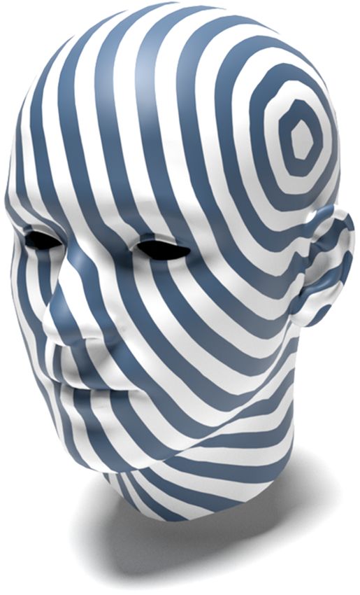
A. Bunge, P. Herholz, M. Kazhdan, M. Botsch / Polygon Laplacian Made Simple
The product of divergence and gradient gives the stiffness matrix
S = D · G = −GT · M
e ·G (5)
and the Laplacian becomes
L = −M−1 · GT · M
e · G. (6)
In practice, the mass matrix is often approximated by a diagonal
(lumped) mass matrix with the i-th diagonal entry in the lumped
matrix set to the sum of entries in the i-th row of the original matrix. Figure 1: Spanned triangle fan on the virtual mesh after inserting
This makes inversion of M straightforward. the virtual vertex x|V |+ j at the j-th face.
The Galerkin method
Assume that we are given two finite-dimensional nesting function
We propose an in-between approach – introducing a virtual ver-
spaces F c ⊂ F f . Given a prolongation operator P injecting the
tex in the middle of each face, expressed as the affine combination
coarser space into the finer, P : F c ,→ F f , and given a symmetric
of the face’s vertices. Naively, the new vertex produces a refined
positive semi-definite operator Q defining a quadratic energy on
triangle mesh with a finite elements system given by the hat basis
the space of functions, we can define a symmetric positive semi-
functions, as before. However, we then coarsen the refined system,
definite operator on the space F f through restriction
expressing the vertex functions on the coarse mesh as linear com-
Q f (φ, ψ) := Q(φ, ψ), ∀φ, ψ ∈ F f . (7) binations of the hat basis functions on the finer one.
In a similar manner, we can define a symmetric positive semi- This new system has dimension equal to the number of vertices
definite operator Qc on the space F c . in the original polygon mesh (preserving the finite elements system
dimension) and has the property that basis functions have overlap-
The Galerkin method tells us that the operators are related by
ping support only if the associated vertices lie on a common face
Qc = P∗ ◦ Q f ◦ P, (8) (defining a sparse system that preserves the symmetry structure). A
further advantage of our approach is that we easily obtain a con-
where P∗ is the dual of P. In particular, given bases for F c and F f sistent factorization of the stiffness matrix as the product of diver-
and letting P, Qc , and Q f be the matrices representing the operators gence and gradient matrices.
with respect to these bases, we have
Qc = PT · Q f · P. (9)
4.1. Construction of the finite elements system
Given a polygon mesh M = (V, F), we construct our finite ele-
4. Polygon Laplacian
ments system by defining a refined triangle mesh M f = (V f , T f ).
When working with general polygon meshes, the finite elements Vertices in the refined mesh, V f , are obtained by introducing a new
method cannot be applied directly for two reasons. First, when the vertex, v|V |+ j , for every face f j ∈ F and setting the position of
polygon is not planar, it is not clear what the underlying surface is v|V |+ j to an affine combination of the positions of vertices in f j
over which functions should be integrated. Second, even for simple
planar polygons, it is not clear how to associate basis functions with x|V |+ j = ∑ w ji xi , with ∑ w ji = 1. (10)
vi ∈ f j vi ∈ f j
the vertices of the mesh.
A simple approach would be to triangulate all the polygons, Triangles in the refined mesh, T f , are obtained by replacing each
defining a piecewise-linear integration domain, and use the hat ba- face f j ∈ F with the triangle fan connecting the inserted vertex
sis functions to define the finite elements. This would have the v|V |+ j to the edges in f j , as can be seen in Figure 1.
advantage of defining a finite elements system whose dimension
Using the refined triangle mesh, we can define the stiffness ma-
equals the number of vertices in the input mesh. Unfortunately, f f
the introduction of diagonal edges would also break the symmetry trix, S f ∈ R|V |×|V | , using the standard cotangent weights of
structure of the polygonization (e.g., in quad meshes where edges Equation (3). Aggregating the affine weights, we get the prolon-
f
are aligned with principal curvature directions). gation matrix P ∈ R|V |×|V | , with
An alternate approach would be to refine the polygon mesh by 1
if i = j ,
introducing a new vertex in the middle of each face. This would Pi j = wki if i = |V | + k and v j ∈ fk , (11)
preserve the symmetry structure, but would come at the cost of an
0 otherwise .
increase in the finite elements system dimension. Also, as we show
in Section 5, such an approach can result in poor performance due And finally, using the Galerkin method, we obtain an expression
to the introduction of negative edge weights in the stiffness matrix. for the coarsened polygonal stiffness matrix as
(For example, refining a rectangle by adding the mid-point creates
two triangles with angles larger than π/2.) S = PT · S f · P. (12)
c 2020 The Author(s)
Computer Graphics Forum c 2020 The Eurographics Association and John Wiley & Sons Ltd.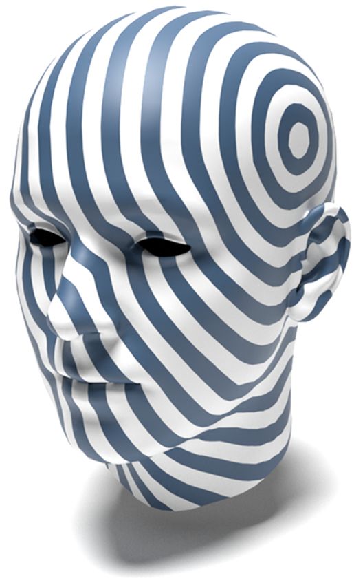
A. Bunge, P. Herholz, M. Kazhdan, M. Botsch / Polygon Laplacian Made Simple

We use the same approach to obtain the coarsened polygonal mass               centroid, the minimizer of the squared area tends to be positioned
matrix M, but in addition to restricting the refined triangle mass            in the interior of the polygon, even when the polygon is not convex.
matrix M f , we also lump it to a diagonal matrix:                               While the position of our virtual vertex is unique, its expres-

                       M = lump PT · M f · P       with       (13)            sion as the linear combination of polygon vertices usually is not.
                            (                                                 Since linear precision requires x f to be an affine combination of
                                ∑k Mik if i = j ,                             the polygon’s vertices (see Section 4.3), finding the position of the
              lump(M)i j =                                    (14)            virtual vertex can be formulated as a minimization directly over the
                                   0     otherwise ,
                                                                              weights w = (w1 , . . . , wn )T :
setting the diagonal entry to the sum of the entries in the row.                                                                    !2
                                                                                                                 n                       n
   We note that our stiffness matrix has non-zero entries if the cor-                       w f = arg min ∑ area xi , xi+1 , ∑ w j x j
                                                                                                            w
responding vertices share a face, not just an edge. We also note that                                           i=1                     j=1
                                                                                                                                                                 (16)
solving a linear system using our operators is different from solving                                                 n
the system on the refined mesh and only using the solution values                                    such that       ∑ w j = 1.
                                                                                                                     j=1
at the original (i.e., non-virtual) vertices. Our approach corresponds
to solving the system using a coarser function space. The alterna-            Noting that when n > 3 the system is under-constrained (with mul-
tive corresponds to sub-sampling a solution obtained over a refined           tiple affine weights defining the same unique squared-area mini-
function space, which could result in aliasing.                               mizer x f ), we add the constraint that, of all the weights w defining
                                                                              the minimizing position x f , we prefer the one with minimal L2 -
                                                                              norm kwk. This encourages the weights to be as uniform as pos-
4.2. Choice of virtual vertex position                                        sible, allowing each polygon vertex to contribute equally. These
Choosing different virtual vertex positions, we provide a frame-              affine weights can be obtained by solving a single linear system,
work for defining a whole family of polygon Laplace operators.                derived in Appendix A.
While many choices are possible we would like the virtual vertex                 It is tempting to add non-negativity constraints w j ≥ 0 to Equa-
to fulfill a set of properties in order to yield a geometric Laplacian:       tion (16) since this would yield convex weights that guarantee a
• The vertex should be efficient to compute and uniquely defined.             maximum principle for the virtual vertex and prevent negative co-
• Since the choice of virtual vertex defines the surface of the poly-         efficients in the coarsened stiffness matrix S (see Equation (12)) as
  gon, we would like to find a point giving small surface area.               long as they do not appear in S f . However, this comes at the cost
• For planar polygons, the vertex should be inside the polygon.               of solving a quadratic program with inequality constraints.
• To achieve linear precision, the virtual vertex should be an affine            We compare our choice of virtual vertex—minimizing the sum
  combination of polygon vertices (see Equation (10)).                        of squared triangle areas through affine weights—to the other op-
                                                                              tions (centroid, min. area, convex weights) in Section 5.7.
  A straightforward choice is to use the centroid of the polygon
vertices. However, for non-convex (planar) polygons this point can
be located outside the polygon. Moreover, it will be biased by an             4.3. Properties of the operator
uneven distribution of polygon vertices.                                      One goal of our construction is to preserve the beneficial numeri-
   Another choice is to find a point minimizing the area of the               cal properties of the cotangent Laplacian. Symmetry and negative
induced triangle fan, which is related to the minimization of the             semi-definiteness follow directly from our construction of the stiff-
Dirichlet energy. Unfortunately, this point is not uniquely defined.          ness matrix S = PT · S f · P, since the refined (cotangent) stiffness
For example, for convex planar polygons, the total area will be               matrix S f has these properties and since the prolongation matrix P
identical for every virtual vertex inside the polygon. Furthermore,           has full rank. (Note that Wardetzky and Alexa [WMKG07, AW11]
since area is non-linear in the position of the virtual vertex, less ef-      aim for positive definiteness, since they define their geometric
ficient iterative solvers, e.g. Newton’s method, are required to com-         Laplacian as the negative of ours.)
pute the position of the virtual vertex.                                         For linear precision we require (S · u)i = 0 whenever vertex vi is
   Instead, we opt for the minimizer of the sum of squared triangle           not part of the boundary, all incident polygons f j 3 vi are coplanar,
areas of the induced triangle fan. Introducing a virtual vertex with          and the values of u in the one-ring of vi are obtained by sampling
position x f into an n-gon with vertex positions (x1 , . . . , xn ) allows    a linear function on the plane. To see that this is the case, we note
us to define the triangle fan with n triangles (xi , xi+1 , x f ), where      that by constraining ourselves to use affine weights in defining the
indices are interpreted modulo n. The position of the virtual vertex,         prolongation, we ensure that prolonging u to the finer mesh, the
x f ∈ R3 , is then defined as the minimizer                                   values of u f = P · u sample a linear function at all vertices of the
                                                                              fan triangulations incident to vi . Since the cotangent Laplacian has
                                 n                      2                    linear precision, this implies that S f · u f is zero at vi and all virtual
                 x f = arg min ∑ area xi , xi+1 , x f        .       (15)
                            x
                                i=1
                                                                              centers v|V |+ j with f j 3 vi . Since these are precisely the entries at
Compared to the minimizer of the area, the squared area mini-                 which the i-th column of P is non-zero, it follows that (PT · S f ·
mizer has two advantages. First, the solution is unique even for              u f )i = 0. Or, equivalently, (S · u)i = 0.
planar convex polygons. Second, using the squared area, the ob-                 It follows that if the initial mesh M is a triangle mesh, then the
jective function becomes quadratic in x f . Also, in contrast to the          derived stiffness matrix S is the standard cotangent Laplacian. This

                                                                                                                                                  c 2020 The Author(s)
                                                                                 Computer Graphics Forum c 2020 The Eurographics Association and John Wiley & Sons Ltd.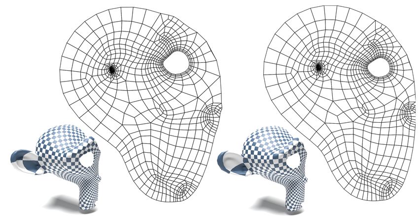
A. Bunge, P. Herholz, M. Kazhdan, M. Botsch / Polygon Laplacian Made Simple
is because using affine weights, the finite elements basis defined on Note that the derived gradient operator, G = G f · P, is a map from
the coarse mesh through prolongation is precisely the hat basis. functions defined on the vertices of the original polygon mesh to
tangent vector fields that are constant on triangles of the refined
The property of positive off-diagonal values does not hold for
mesh. These refined triangles, however, can uniquely be identified
the cotangent Laplacian and consequently cannot extend to our
with half-edges of the original polygon mesh, so that the refined tri-
construction, resulting in the potential violation of the maximum
angles never have to be constructed explicitly. Hence, the gradient
principle. The lack of positivity is also present in the definition
operator maps from function values at vertices to vectors at half-
of [AW11], however, our operator tends to contain fewer negative
edges (and conversely for the divergence operator, D = P> · D f ).
off-diagonal coefficients (see Section 5).
4.6. Finite Elements Exterior Calculus
4.4. Implementation
An alternative approach is to define differential operators by ex-
Implementing our system is simple, especially if code for the com- tending Finite Elements Exterior Calculus to polygon meshes. We
putation of the cotangent Laplacian is already available. Our im- do this by using our coarsened basis to define Whitney bases for
plementation is based on the PMP-Library [SB19]. Algorithm 1 higher-order forms and then using these higher-order bases to de-
illustrates the procedure. Initially we set the prolongation matrix P fine the Hodge star operators.
to the identity of size |V | × |V | (line 3), reflecting the fact that all
original vertices appear in the refined mesh. We then loop over all Recall Given a basis of zero-forms {ψi } forming a partition of
faces, collecting all vertex positions of the polygon, finding affine unity, one can define Whitney bases [Whi57, AFW06] for 1-forms
weights for the optimal virtual vertex, and constructing this point {ψi j } (with i < j and supp(ψi )∩supp(ψ j ) 6= ∅) and 2-forms {ψi jk }
(lines 5–7, Section 4.2). Next we compute the area and cotangent (with i < j < k and supp(ψi ) ∩ supp(ψ j ) ∩ supp(ψk ) 6= ∅) by set-
weights for the resulting triangle fan and aggregate them in M f ting:
and S f (lines 9–10, Section 3). The final operators are constructed
by multiplying the matrices M f and S f defined on the refined mesh ψi j = ψi · dψ j − ψ j · dψi ,
with the prolongation matrix and its transpose (line 12, Section 4.1). ψi jk = 2 ψi · dψ j ∧ ψk − ψ j · dψi ∧ dψk + ψk · dψi ∧ dψ j .
The exterior derivatives are then defined using the combinatorics
Algorithm 1: Assemble polygon stiffness and mass matrix
1 i = l, j = m
Data: Mesh vertices V and faces F −1 i = k
1 j = l, k = m
0 1
Result: Mass matrix M, stiffness matrix S. d(i j)k = 1 j=k , d(i jk)(lm) =
f |V f |×|V f |
−1 i = l, k = m
0 otherwise
1 S =0
0 otherwise
f f
2 M f = 0|V |×|V | (19)
3 P = I|V |×|V | and the discrete Hodge stars are defined using the geometry
4 foreach f ∈ F do
5 X ← getVertexPositions( f ); ? 0i j = hhψi , ψ j ii, (20)
6 w ← findVirtualVertexWeights(X); ? 1(i j)(kl) = hhψi j , ψkl ii, (21)
7 x ← XT · w;
8 P ← appendWeightRow(P, f , w); ? 2(i jk)(lmn) = hhψi jk , ψlmn ii, (22)
9 M f ← M f + buildTriangleFanMassMatrix( f , X, x); with hh·, ·ii denoting the integral of the (dot-)product of k-forms.
10 S f ← S f + buildTriangleFanCotan( f , X, x); Using the hat basis on a triangle mesh, the basis functions are lin-
11 end ear within each triangle so computing the coefficients reduces to
integrating quadratic polynomials over a triangle.
12 return M = PT · M f · P, S = PT · S f · P
Prolonging higher-order forms Given the hat basis on the refined
f f
triangle mesh {φ1 , . . . , φ|V f | }, defining a prolongation operator P
4.5. Gradient and divergence is equivalent to defining a coarsened basis {φ1 , . . . , φ|V | } on the
f
We are also able to factor the stiffness matrix as the product of di- triangle mesh, with φ j = ∑i Pi j φi .
vergence and gradient matrices. As described in Section 3, we can As both bases form a partition of unity, we can define Whitney
obtain a matrix expression for the gradient and divergence opera- bases for higher-order forms. In doing so we get:
tors over the refined mesh, G f and D f and use those to factor the f f
refined triangle stiffness matrix φi j = ∑ Pki Pl j φkl and φi jk = ∑ Pli Pm j Pnk φlmn , (23)
k,l l,m,n
Sf = Df ·Gf . (17)
which gives prolongation operators for 0-, 1-, and 2-forms:
Coarsening, we obtain a factorization of the polygon stiffness ma-
P0i j = Pi j , (24)
trix in terms of coarse polygon divergence and gradient matrices
T P1(i j)(kl) = Pik · P jl , (25)
S=P · D }f · G f
| {z· P} . (18)
P2(i jk)(lmn)
| {z
=D =G = Pil · P jm · Pkn . (26)
c 2020 The Author(s)
Computer Graphics Forum c 2020 The Eurographics Association and John Wiley & Sons Ltd.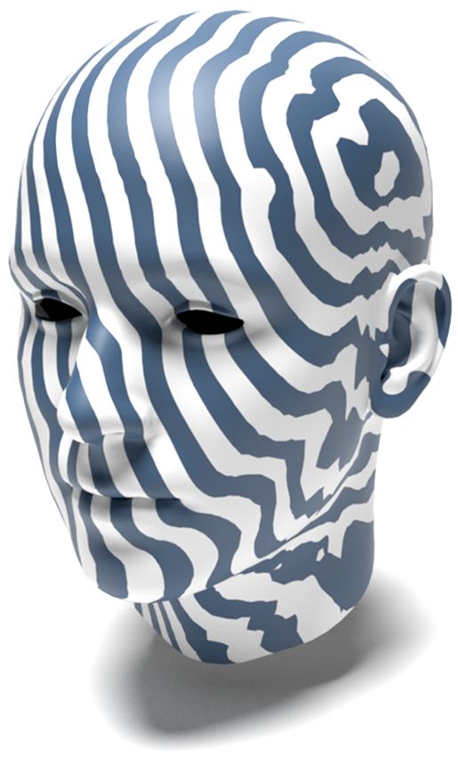
A. Bunge, P. Herholz, M. Kazhdan, M. Botsch / Polygon Laplacian Made Simple
This allows us to define Hodge star operators for the coarsened
basis through prolongation:
? k = (Pk )T · ? k, f · Pk , (27)
k
where ? is the discrete Hodge star for k-forms defined using the
coarsened basis and ? k, f is the discrete Hodge star for k-forms de-
fined using the refined hat basis. R EGULAR S PHERE N OISY S PHERE
In particular, this gives a factorization of the stiffness matrix as
S = −(d0 )T · ?1 · d0 , with gradients represented in terms of dif-
ferences across polygon edges/diagonals. The minus sign is due to
our design choice of a negative semi-definite stiffness matrix, as
discussed in Section 3.
5. Evaluation H EX S PHERE F INE S PHERE
We evaluate our Laplacian in a variety of different geometry pro-
Figure 2: Spherical meshes used for testing the accuracy of spher-
cessing operations, applied to a selection of polygon meshes (Fig-
ical harmonics and mean curvature.
ures 2 and 3). These results are compared to two other methods.
First, we triangulate each (potentially non-planar, non-convex) n-
gon into n − 2 triangles without inserting an extra point, and then
use the standard cotangent Laplacian for triangle meshes. Using the
dynamic-programming approach of Liepa [Lie03] we find the poly-
gon triangulation that minimizes the sum of squared triangle areas
(similar in concept to our squared area minimization). We also ex- Q UADS 1 Q UADS 2 L-S HAPED T ETRIS 1 T ETRIS 2
perimented with the triangulation that maximizes the minimum tri-
angle angle (similar to planar Delaunay triangulations). While the Figure 3: Planar meshes used for the evaluation of geodesic dis-
latter yields better-behaved cotangent weights, it tends to produce tances, including non-convex and non-star shaped tessellations.
flips or fold-overs for non-convex polygons, so we used the for-
mer for most experiments. Second, we compare our results to the
ones obtained with the polygon Laplacian of Alexa and Wardet-
zky [AW11], based on their original implementation, using various
values for their parameter λ that assigns weight to the component
perpendicular to the projection direction.
5.1. Conformalized mean curvature flow
A common approach for smoothing meshes is to use implicit in-
tegration to solve the diffusion equation [DMSB99]. In our appli- Figure 4: Stress test for smoothing on a noisy sphere (left). After
cation we use the conformalized Mean Curvature Flow introduced one (center) and ten iterations (right).
by Kazhdan et al. [KSBC12], which obtains the coordinates of the
mesh vertices at the next time-step, Xt+ε from the coordinates at
the current time-step, Xt , iteratively solving the linear system
Mt − εS0 Xt+ε = Mt Xt (28)
with ε the time-step, S0 the initial stiffness matrix, and Mt the mass
matrix at time t. After each iteration the mesh is translated back to
the origin and re-scaled to its original surface area. Figure 4 demon-
strates the resilience of our Laplacian to noise and non-planar as
well as non-convex faces. The flow can recover the spherical shape
after one iteration and converges after 10 iterations.
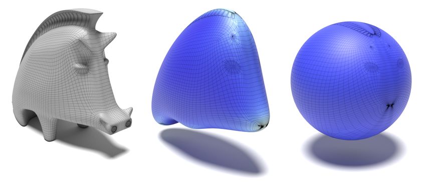
Figure 5 shows an example of this flow after one and ten iter-
Figure 5: Visualization of the mean curvature flow on a quad mesh.
ations respectively. The mean curvature is color-coded and shows
Mean curvature is color coded.
that the mesh correctly converges to a sphere when using our oper-
ator. This example shows that even extreme differences in polygon
scale are handled correctly. The results of Alexa and Wardetzky’s
c 2020 The Author(s)
Computer Graphics Forum c 2020 The Eurographics Association and John Wiley & Sons Ltd.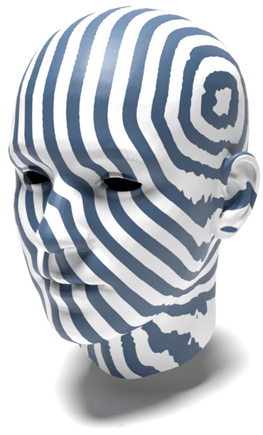
A. Bunge, P. Herholz, M. Kazhdan, M. Botsch / Polygon Laplacian Made Simple

                                     Ours                 [AW11]
                                              −3
                Figure 4       5.075 × 10             5.417 × 10⁻³
                Figure 5       2.271 × 10⁻³            2.69 × 10⁻³
                Figure 6       1.157 × 10⁻³           1.204 × 10⁻³

Table 1: Conformal distortion of conformal spherical [KSBC12]
and spectral free-boundary [MTAD08] parametrizations.

                                                                    [AW11]
 Mesh                           Ours       [Lie03] λ = 0.1 λ = 0.5                 λ=1
 R EGULAR S PHERE             0.0168       0.0469       0.0290        0.0290      0.0290   Figure 6: Parametrization of the right half of a quadrangulated
 N OISY S PHERE               0.0469       0.1053       0.0562        0.0814      0.1551   monkey head. The result of [AW11] (left) is similar to ours (right),
 H EX S PHERE                 0.0016       0.3711       0.0023        0.0038      0.0075   but our operator has slightly lower conformal distortion.
 F INE S PHERE                0.1334       0.0623       0.0279        0.0107      0.0141

Table 2: Root-mean-square error (RMSE) of the curvature devia-
tion for different meshes of the unit sphere.
                                                                                           5.4. Reproducing the spherical harmonics

                                                                                           The eigenfunctions of the Laplacian form an orthonormal basis
operator are qualitatively very similar, however, analyzing the con-                       known as the “manifold harmonics” [VL08]. In the case that the
formal error shows a small advantage for our method (see Table 1).                         surface is a sphere, these eigenfunctions are known to be the spher-
We evaluated the conformal distortion by computing the root mean                           ical harmonics. We evaluate the quality of our Laplacian by mea-
square errors of area-weighted angle differences between the mesh                          suring the extent to which the true spherical harmonics are eigen-
and its spherical parametrization. We opted for this measure be-                           vectors of the Laplacian.
cause it is not obvious how to compute conformal distortion for
non-planar polygons.                                                                          We know that the spherical harmonic Ylm : S2 → R is an eigen-
                                                                                           function of the Laplacian with eigenvalue −l · (l + 1). Sampling
                                                                                                                                                      |V |
                                                                                           Ylm at the vertices of the spherical mesh, we obtain ym
                                                                                                                                                 l ∈ R . We
5.2. Mean curvature estimation                                                             measure the accuracy of our Laplacian by evaluating
Noting that the Laplacian of the coordinate function is the mean-                                                                            2
curvature normal vector, we can use our Laplace operator to ap-                                                               1
                                                                                                                 ym
                                                                                                                  l +               L · ym
                                                                                                                                         l       ,               (30)
proximate the mean curvature H at vertex vi                                                                             l · (l + 1)          M
                       1                                                                  with the L2 -norm computed relative to the mass matrix M.
             H(vi ) :=    (LX)i · sign (LX)i , ni               (29)
                       2
with X the matrix of vertex coordinates and ni the normal at vi .                             Table 3 compares the spectral error, giving the sum of errors over
                                                                                           the spherical harmonics in the first nine frequencies (1 ≤ l ≤ 9).
   Since the mean curvature is 1 at every point on the unit sphere,                        As the table shows, in this experiment we are unable to reproduce
we can measure the accuracy of our Laplacian by comparing the es-                          the accuracy of Alexa and Wardetzky’s Laplacian. However, our
timated mean curvature to the true one. Table 2 gives the root mean                        construction does not require selecting a parameter on a case-by-
square error (RMSE), comparing curvature estimates over differ-                            case basis as in [AW11].
ent polygonizations of the sphere, and using different definitions of
the Laplace operator. As the table shows, our operator outperforms
existing methods on most spherical meshes.

                                                                                                                                                     [AW11]
5.3. Parametrization
                                                                                           Mesh                    Ours      [Lie03] λ = 0.1 λ = 0.5           λ=1
We compare our operator to [AW11] with respect to conformal
                                                                                           R EGULAR S PHERE       0.0393     0.0200     0.0599       0.0220    0.0175
parametrization based on Mullen et al.’s [MTAD08] spectral free-
                                                                                           N OISY S PHERE         0.0643     0.0722     0.0969       0.0589    0.1366
boundary parametrization. Figure 6 illustrates that both operators
                                                                                           H EX S PHERE           7.41e-7    0.0037     9.93e-6      1.46e-6   1.13e-6
perform well for this quad mesh. In this case we obtain a confor-
                                                                                           F INE S PHERE          0.0003     6.73e-5    0.0005       6.48e-5   8.98e-5
mal distortion (c.f. Section 5.1) of 1.157 × 10⁻³ while the method
of [AW11] achieves 1.204 × 10⁻³ . For [AW11] we systematically                             Table 3: We measure the extent to which the spherical harmonics of
tried to find the best parameter λ and consistently observed very                          frequencies 1 ≤ l ≤ 9 are eigenvectors, with eigenvalue −l · (l + 1),
similar behavior with a slightly lower conformal distortion for our                        of the Laplacian on spherical meshes.
operator, across a variety polygon meshes.

 c 2020 The Author(s)
Computer Graphics Forum c 2020 The Eurographics Association and John Wiley & Sons Ltd.
A. Bunge, P. Herholz, M. Kazhdan, M. Botsch / Polygon Laplacian Made Simple

        a) ours               b) [AW11]              c) refinement           d) max-angle                     e) min-area              f) intrinsic Delaunay
Figure 7: Computing geodesic distances on a quad mesh (top left) following the approach of Crane et al. [CWW13], using our operator
(a) and Alexa and Wardetzky’s (b, using λ = 0.5). Images (c–f) show results using different triangulation strategies: refining the mesh by
inserting the virtual point (c), triangulating polygons to maximize the minimum angle (d), and triangulating polygons to minimize squared
triangle areas (e). To improve the results of (e), we employ the Laplacian based on the intrinsic Delaunay triangulation [BS07] (f). The
triangles of (d) are already Delaunay, therefore using the intrinsic triangulation does not further improve the result in (d).

5.5. Geodesics in Heat                                                        We qualitatively compare the results using our operator, the one
                                                                           from [AW11], and several polygon triangulation strategies in Fig-
In [CWW13], Crane et al. proposed the heat method for computing
                                                                           ure 7. (a) Our construction gives a result with considerably fewer
geodesic distances from a selected vertex vi to all others on the
                                                                           artifacts compared to the other approaches. (b) The Laplace op-
mesh. Let D be the divergence operator, G the gradient operator and
         c                                                                 erator of Alexa and Wardetzky fails independent of the choice of
ei ∈ R|V | the i-th unit vector. The geodesic distances are computed
                                                                           λ. (d) Triangulating polygons to maximize the minimal angle also
in four steps.
                                                                           gives good results, but this approach is not suitable for arbitrary
  First, the impulse function ei is diffused for a time-step of ε by       meshes since it fails on non-convex polygons. (e) Minimum-area
solving for u ∈ R|V | such that                                            triangulations avoid this problem, but give worse results due to poor
                                                                           triangle shapes. (f) Combining minimum-area triangulations with
                       (M − εS) u = M · ei ,                    (31)       the Laplacian based on the intrinsic Delaunay triangulation [BS07]
where we set ε to the squared mean of edge lengths as suggested in         fixes this problem, but is more complex to compute. In (c) we show
[CWW13]. Next, the gradients of u are computed and normalized              the result obtained by using the cotangent Laplacian on the mesh
                                                        f
to have unit length, resulting in a vector field g ∈ R|T |×3 with          explicitly refined by inserting the virtual vertices (this is equiva-
                                                                           lent to S f ). Our construction is clearly different from just refining
                                  (G · u)i                                 polygons.
                         gi = −            .                    (32)
                                  (G · u)i
                                                                              The quality of geodesics is linked to the number of negative off-
Finally, the geodesic distance, d ∈ R|V | is computed by solving for       diagonal coefficients in the stiffness matrix. Analyzing the ratio of
the scalar field whose gradient best matches g                             negative off-diagonal entries for Figure 7 confirms this correlation:
                            S·d = D·g                           (33)
                                                                                         ours      [AW11]           c)        d)        e)        f)
and additively offsetting so that it has value zero at vi . Our poly-
gon Laplacian offers a natural decomposition into divergence and                        11%          21%          17%        5%       15%        0%
gradient (c.f. Section 4.5). Crane et al. [CWW13] demonstrate how
to obtain a normalized gradient for computing geodesic distances           We consistently observe a significantly smaller number of negative
using the operator of Alexa and Wardetzky.                                 off-diagonal coefficients in our operator as compared to [AW11].

                                                                                                                                               c 2020 The Author(s)
                                                                              Computer Graphics Forum c 2020 The Eurographics Association and John Wiley & Sons Ltd.
A. Bunge, P. Herholz, M. Kazhdan, M. Botsch / Polygon Laplacian Made Simple

                                                               [AW11]                    Laplacian is faster than defining a polygon Laplacian. Also, since
                                                                                         a vertex on the polygon mesh has at least as many face-adjacent
  Mesh                 Ours        [BS07]        λ = 0.1        λ = 0.5         λ=1      neighbors as the same vertex on the triangulated mesh, the polygon
  Q UADS 1            0.0265       0.0394         0.0179         0.0415        0.1206    Laplacians are less sparse, resulting in an increased solver time.
  Q UADS 2            0.0356       0.0856         0.0403         0.0469        0.1233
  L-S HAPED           0.0574       0.0736         0.4216         0.1115        1.6531
  T ETRIS 1           0.2183       0.1408         0.4521         0.2304        0.2483    5.7. Comparison of virtual vertex choices
  T ETRIS 2           0.0821       0.0665         0.4381         0.1177        0.1852    As stated in Section 4.2, there are several options for computing the
                                                                                         virtual vertices and their weights. We compare the performance of
Table 4: Root-mean-square error of computed geodesic distances
                                                                                         these alternative constructions, using both lumped and un-lumped
for the different planar tessellations shown in Figure 3.
                                                                                         mass matrices, in a number of applications. For geodesic distances
                                                                                         (see Section 5.5), our proposed version using affine weights gives
Mesh             Affine Convex Centroid Abs. Area [AW11] [Lie03]                         the overall best results (see Table 6), although the strictly con-
                                                                                         vex weights yield a smaller error for meshes with non-star-shaped
H EXAGON            55         142          13            357           52          21   faces. For most applications, using the lumped mass matrix gives
Q UADS             171         573          50           1460          240          82   better results, as also shown in the additional experiments in the
H EXAGON 472+25 483+25 476+26                          469+25        477+26 77+8         supplementary material. Balancing numerical performance with
Q UADS   596+35 596+35 599+35                          600+36        599+35 498+29       efficiency, we found the minimizer of the squared triangle areas
                                                                                         through affine weights to be the best choice.
Table 5: Timing (in ms) for constructing the Laplace matrix (top)
and solving the linear system (bottom). The latter is split into the
time needed for Cholesky factorization and for back-substitution.                        5.8. Convergence behavior
                                                                                         We evaluate the convergence behavior of our Laplacian under mesh
                                                                                         refinement by solving the Poisson equation ∆ f = b with Dirichlet
Moreover, the optimal λ parameter for [AW11] has to be deter-                            boundary conditions for the Franke test function [Fra79]
mined manually for each mesh.
                                                                                                           3 (9x−2)2 +(9y−2)   2
                                                                                                                                  3 (9x+1)2 9y+1
   Figure 8 shows another result of geodesics in heat. This example                              f (x, y) = e−          4        + e− 49 − 10
                                                                                                           4                      4
features highly anisotropic polygons that lead to severe distortions                                       1 − (9x−7)2 +(9y−3)2
                                                                                                                                  1        2       2

for [AW11], while our operator defines smooth geodesic distances.                                         + e          4         − e−(9x−4) −(9y−7) .
                                                                                                           2                      5
   Table 4 provides a quantitative evaluation of geodesic distances,                     Figure 9 depicts the decrease of the L2 error under mesh refinement
by compare them to Euclidean distances on different planar meshes                        for regular triangle, quad, and hex meshes. The identical slope in
(Figure 3). Our operator yields smaller root-mean-square errors for                      this log-log plot reveals that our operator inherits the quadratic con-
most models, including the geodesic distances computed via intrin-                       vergence order of the triangle-based cotangent Laplacian.
sic Delaunay triangulation [BS07,SSC19] (based on the implemen-
tation provided in libigl [JP∗ 18]).                                                     Summary While our evaluations do not demonstrate that our
                                                                                         Laplace operator is superior to existing state-of-the-art methods, it
5.6. Timings                                                                             does show that it is competitive. We perform slightly better than tri-
                                                                                         angulation [Lie03]. This is likely because our Laplacian is denser.
We evaluated the computational costs of the different operators                          And, while the polygon Laplacian of [AW11] outperforms ours in
on the H EX S PHERE (16070 faces) and the F INE S PHERE (96408                           some cases, its behavior depends on the choice of the parameter λ,
faces) shown in Figure 2. All timings were measured on a standard                        which cannot be fixed so as to perform well in all cases. In contrast,
workstation with a six-core Intel Xeon 3.6 GHz CPU; no experi-                           our method is parameter-free.
ment exploited multi-threading. We analyze our approach with the
different virtual vertex options described in Section 4.2: centroid of
polygon vertices, minimizing the sum of (absolute) triangle areas                        6. Conclusion
(Abs. Area), minimizing the sum of squared triangle areas using ei-
                                                                                         In this work we have proposed a novel polygon Laplacian, defined
ther affine weights or convex weights. We compare these methods
                                                                                         by first refining the polygon mesh to a triangle mesh and then coars-
to Alexa and Wardetzky [AW11] and to the minimum area polygon
                                                                                         ening the cotangent Laplacian from the triangle mesh back to the
triangulation [Lie03]. The timings are given in Table 5.
                                                                                         original polygon mesh. The derived polygon Laplacian exhibits nu-
   In terms of the construction time for the Laplace matrix, our ap-                     merous desirable properties including sparsity, symmetry, negative
proach is faster than [AW11] on fine-resolution meshes and com-                          semi-definiteness, linear precision, and consistency with the diver-
parable for coarser meshes. And, with the exception of centroid, it                      gence and gradient operators, without suffering from an increase
is also the fastest of the different virtual vertex choices, since the                   in the dimensionality of the linear system. We have evaluated our
Newton optimization of Abs. Area (based on Eigen) and the QP                             Laplacian against other state-of-the-art methods and have demon-
solver of convex (based on CGAL) are computationally expensive.                          strated that it performs competitively, providing efficient and high-
However, triangulating the mesh and constructing the cotangent                           quality solutions without requiring parameter tuning.

 c 2020 The Author(s)
Computer Graphics Forum c 2020 The Eurographics Association and John Wiley & Sons Ltd.
A. Bunge, P. Herholz, M. Kazhdan, M. Botsch / Polygon Laplacian Made Simple

                                   a)                                          b) ours                                                c) [AW11]
Figure 8: Geodesic distances computed on a quad mesh (a) with our Laplacian (b) and the Laplacian proposed in [AW11] (c). Even with the
manually determined best weight parameter (λ = 0.4), (c) exhibits distortions while ours remains stable despite highly anisotropic faces.

                                             un-lumped mass matrix                                           lumped mass matrix
             Mesh              Affine     Convex    Centroid    Abs.Area                     Affine        Convex    Centroid   Abs.Area
             Q UADS 1          0.025       0.025         0.025             0.025             0.026          0.027            0.027              0.027
             Q UADS 2          0.031       0.031         0.031             0.031             0.036          0.036            0.036              0.036
             L-S HAPED         0.141       0.165         0.134             0.134             0.057          0.063            0.068              0.068
             T ETRIS 1         0.465       0.490         0.490             0.491             0.218          0.181            0.186              0.185
             T ETRIS 2         0.406       0.346         0.151             0.153             0.082          0.089            0.089              0.088

Table 6: RMSE of geodesic distances for the planar meshes in Figure 3 computed with different choices of virtual vertices and using un-
lumped and lumped mass matrices.

                                                                                   Appendix A: Finding the optimal virtual point
                                                                                   Given a polygon with n vertices (x1 , . . . , xn ), we want to insert a
                                                                                   point x = x(w), defined as an affine combination x(w) = ∑nj=1 w j x j
                                                                                   with ∑ j w j = 1, such that the sum of squared triangle areas over
                                                                                   the resulting triangle fan is minimized. This leads to the following
                                                                                   optimization problem in the weights w = (w1 , . . . , wn )T :
                                                                                                                       !2
                                                                                              n                       n                          n
                                                                                       min ∑ area xi , xi+1 , ∑ w j x j                 s.t.    ∑ w j = 1.           (34)
                                                                                         w
                                                                                             i=1                      j=1                       j=1

                                                                                   The objective function can be rewritten as
                                                                                                             n
                                                                                                                  1
Figure 9: L2 convergence plots for the solution of the Poisson equa-
                                                                                                  E(w) =    ∑ 2 k(xi − xi+1 ) × (x(w) − xi )k2 .                     (35)
                                                                                                            i=1
tion on triangle, quad, and hex meshes of increasing resolution.
                                                                                   Since E is quadratic in x(w) and therefore also quadratic in w, it
                                                                                   can be written as
                                                                                                              1
   In the future, we would like to extend our approach in several                                    E(w) = wT Aw + bT w + c.                   (36)
                                                                                                              2
ways. We would like to consider introducing multiple virtual ver-                                                                         ∂E
tices within a single face as this could allow for better triangulations           Minimizing with respect to w, i.e., setting            ∂w
                                                                                                                                               to zero, leads to
of non-convex polygons. We would like to consider loosening the                         Aw = −b          with
restriction that the virtual vertex needs to be an affine combination
of the polygon vertices. For example, in the case of a planar poly-                               n
gonization of the sphere, this would allow us to introduce vertices                      Ai j = 2 ∑ x j × (xk+1 − xk ) · (xi × (xk+1 − xk )) ,
                                                                                                                                                                     (37)
                                                                                                   k=1
on the surface of the sphere, not just on the planes containing the
                                                                                                    n
polygons. Finally, we would like to extend our approach to higher-                        bi = 2 ∑ (xi × (xk+1 − xk )) · ((xk+1 − xk ) × xk )
order basis functions and volumetric polyhedral meshes.                                            k=1
                                                                                   We add one row to the matrix to enforce the partition of unity con-
Acknowledgments We thank the anonymous reviewers for their
                                                                                   straint ∑ j w j = 1, turning it into the (n + 1) × n linear system
valuable comments and suggestions, and Marc Alexa and Fabian

Prada for helpful discussions on Laplacians and discrete exterior                                               A             −b
                                                                                                                       w=           .                 (38)
calculus. This work was sponsored in part by NSF Award 1422325.                                               1···1            1

                                                                                                                                                      c 2020 The Author(s)
                                                                                     Computer Graphics Forum c 2020 The Eurographics Association and John Wiley & Sons Ltd.
A. Bunge, P. Herholz, M. Kazhdan, M. Botsch / Polygon Laplacian Made Simple
The matrix A has rank 2 or 3 for planar or non-planar polygons, [GJ∗ 10] G UENNEBAUD G., JACOB B., ET AL .: Eigen v3.
respectively. Hence, the system in Equation (38) has rank 3 or 4 for http://eigen.tuxfamily.org, 2010. 11
planar/non-planar polygons. It is therefore fully determined for ei- [GL89] G OLUB G. H., L OAN C. F. V.: Matrix Computations. Johns
ther (planar) triangles or non-planar quads, and is underdetermined Hopkins University Press, Baltimore, 1989. 11
otherwise. In the latter case, we aim for the least-norm solution, [JP∗ 18] JACOBSON A., PANOZZO D., ET AL .: libigl: A simple C++
i.e., the solution w with minimal kwk, because it distributes the geometry processing library, 2018. https://libigl.github.io/. 9
influence of polygon vertices xi equally. We handle both the fully- [KSBC12] K AZHDAN M., S OLOMON J., B EN -C HEN M.: Can mean-
determined and the under-determined cases in a robust and unified curvature flow be modified to be non-singular? Computer Graphics Fo-
manner through the matrix pseudo-inverse [GL89], which we com- rum 31, 5 (2012), 1745–1754. 2, 6, 7
pute through Eigen’s complete orthogonal decomposition [GJ∗ 10]. [Lie03] L IEPA P.: Filling holes in meshes. In Proceedings of Euro-
graphics/ACM SIGGRAPH Symposium on Geometry Processing (2003),
pp. 200–205. 6, 7, 9
References [LZ10] L ÉVY B., Z HANG H. R.: Spectral mesh processing. In ACM
[Abb84] A BBOT E. A.: Flatland: A Romance of Many Dimensions. See- SIGGRAPH 2010 Courses (2010), pp. 8:1–8:312. 2
ley & Co., 1884. 1 [Mac49] M AC N EAL R.: The Solution of Partial Differential Equations
[AFW06] A RNOLD D. N., FALK R. S., W INTHER R.: Finite element by Means of Electrical Networks. PhD thesis, California Institute of
exterior calculus, homological techniques, and applications. Acta Nu- Technology, 1949. 1
merica 15 (2006), 1–155. 5 [MTAD08] M ULLEN P., T ONG Y., A LLIEZ P., D ESBRUN M.: Spectral
[AW11] A LEXA M., WARDETZKY M.: Discrete Laplacians on general conformal parameterization. Computer Graphics Forum 27, 5 (2008),
polygonal meshes. ACM Transactions on Graphics 30, 4 (2011), 102:1– 1487–1494. 7
102:10. 1, 2, 4, 5, 6, 7, 8, 9, 10 [PP93] P INKALL U., P OLTHIER K.: Computing discrete minimal sur-
[BKP∗ 10] B OTSCH M., KOBBELT L., PAULY M., A LLIEZ P., L EVY B.: faces and their conjugates. Experim. Math. 2 (1993), 15–36. 1
Polygon Mesh Processing. AK Peters, 2010. 2 [SB19] S IEGER D., B OTSCH M.: The polygon mesh processing library,
[BS07] B OBENKO A. I., S PRINGBORN B. A.: A discrete Laplace– 2019. http://www.pmp-library.org. 5
Beltrami operator for simplicial surfaces. Discrete & Computational [SCOL∗ 04] S ORKINE O., C OHEN -O R D., L IPMAN Y., A LEXA M.,
Geometry 38, 4 (2007), 740–756. 2, 8, 9 RÖSSL C., S EIDEL H.-P.: Laplacian surface editing. In Proceedings
[BSW08] B ELKIN M., S UN J., WANG Y.: Discrete Laplace operator of Eurographics Symposium on Geometry Processing (2004), pp. 179–
on meshed surfaces. In Proceedings of Symposium on Computational 188. 2
Geometry (2008), pp. 278–287. 2 [SSC19] S HARP N., S OLIMAN Y., C RANE K.: Navigating intrinsic tri-
[CLB∗ 09] C HUANG M., L UO L., B ROWN B. J., RUSINKIEWICZ S., angulations. ACM Transactions on Graphics 38, 4 (2019). 2, 9
K AZHDAN M.: Estimating the Laplace-Beltrami operator by restrict- [Tau95] TAUBIN G.: A signal processing approach to fair surface design.
ing 3d functions. Computer Graphics Forum 28, 5 (2009), 1475–1484. In Proceedings of ACM SIGGRAPH (1995), pp. 351–358. 2
2
[VL08] VALLET B., L ÉVY B.: Spectral geometry processing with mani-
[CRK16] C HUANG M., RUSINKIEWICZ S., K AZHDAN M.: Gradient- fold harmonics. Computer Graphics Forum 27, 2 (2008), 251–260. 7
domain processing of meshes. Journal of Computer Graphics Tech-
[Whi57] W HITNEY H.: Geometric Integration Theory. Princeton Uni-
niques 5, 4 (2016), 44–55. 2
versity Press, 1957. 5
[CWW13] C RANE K., W EISCHEDEL C., WARDETZKY M.: Geodesics
[WMKG07] WARDETZKY M., M ATHUR S., K ÄLBERER F., G RINSPUN
in heat: A new approach to computing distance based on heat flow. ACM
E.: Discrete Laplace operators: No free lunch. In Proceedings of Eu-
Transactions on Graphics 32, 5 (2013), 152:1–152:11. 2, 8
rographics Symposium on Geometry Processing (2007), pp. 33–37. 2,
[dGDMD16] DE G OES F., D ESBRUN M., M EYER M., D E ROSE T.: Sub- 4
division exterior calculus for geometry processing. ACM Transactions on
[XLH11] X IONG Y., L I G., H AN G.: Mean Laplace-Beltrami opera-
Graphics 35, 4 (2016), 133:1–133:11. 2
tor for quadrilateral meshes. In Transactions on Edutainment V, Pan
[DMA02] D ESBRUN M., M EYER M., A LLIEZ P.: Intrinsic parameter- Z., Cheok A. D., Müller W., (Eds.). Springer Berlin Heidelberg, 2011,
izations of surface meshes. Computer Graphics Forum 21, 3 (2002), pp. 189–201. 2
209–218. 2
[Zha04] Z HANG H.: Discrete combinatorial Laplacian operators for dig-
[DMSB99] D ESBRUN M., M EYER M., S CHRÖDER P., BARR A. H.: Im- ital geometry processing. In Proceedings of SIAM Conference on Geo-
plicit fairing of irregular meshes using diffusion and curvature flow. In metric Design and Computing (2004), pp. 575–592. 2
Proceedings of ACM SIGGRAPH (1999), pp. 317–324. 1, 6
[Dzi88] D ZIUK G.: Finite Elements for the Beltrami operator on arbi-
trary surfaces. Springer Berlin Heidelberg, 1988, pp. 142–155. 1
[Fle84] F LETCHER C.: Computational Galerkin Methods. Computa-
tional Physics Series. Springer-Verlag, 1984. 2
[Flo97] F LOATER M. S.: Parametrization and smooth approximation of
surface triangulations. Computer Aided Geometric Design 14, 3 (1997),
231–250. 2
[Fra79] F RANKE R.: A critical comparison of some methods for inter-
polation of scattered data. Tech. rep., Naval Postgraduate School, 1979.
9
[GGT06] G ORTLER S. J., G OTSMAN C., T HURSTON D.: Discrete one-
forms on meshes and applications to 3d mesh parameterization. Comput.
Aided Geom. Des. 23, 2 (2006), 83–112. 2
c 2020 The Author(s)
Computer Graphics Forum c 2020 The Eurographics Association and John Wiley & Sons Ltd.You can also read