Polynomial-time algorithms for Multimarginal Optimal Transport problems with structure
←
→
Page content transcription
If your browser does not render page correctly, please read the page content below
Polynomial-time algorithms for Multimarginal Optimal Transport
                                                               problems with structure
                                                                     Jason M. Altschuler                 Enric Boix-Adserà

                                                                                        August 10, 2020
arXiv:2008.03006v1 [math.OC] 7 Aug 2020

                                                                                             Abstract
                                                    Multimarginal Optimal Transport (MOT) has recently attracted significant interest due to
                                                its many applications. However, in most applications, the success of MOT is severely hindered
                                                by a lack of sub-exponential time algorithms. This paper develops a general theory about “struc-
                                                tural properties” that make MOT tractable. We identify two such properties: decomposability
                                                of the cost into either (i) local interactions and simple global interactions; or (ii) low-rank inter-
                                                actions and sparse interactions. We also provide strong evidence that (iii) repulsive costs make
                                                MOT intractable by showing that several such problems of interest are NP-hard to solve—even
                                                approximately. These three structures are quite general, and collectively they encompass many
                                                (if not most) current MOT applications. We demonstrate our results on a variety of applications
                                                in machine learning, statistics, physics, and computational geometry.

                                              The authors are with the Laboratory for Information and Decision Systems (LIDS), Massachusetts Institute of
                                          Technology, Cambridge MA 02139. Work partially supported by NSF Graduate Research Fellowship 1122374, a
                                          Siebel PhD Fellowship, and a TwoSigma PhD fellowship.

                                                                                                  1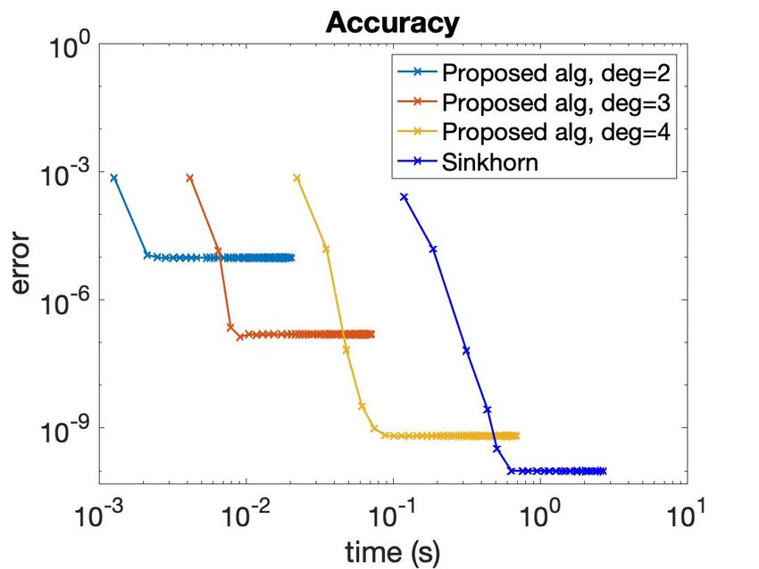
Contents
1 Introduction                                                                                                                                                  3
  1.1 Contributions . . . . . . . . . . . . . . . . . . . . . . . . . . . . . . . . . . . . . . . . . . .                                                       3
  1.2 Techniques . . . . . . . . . . . . . . . . . . . . . . . . . . . . . . . . . . . . . . . . . . . . .                                                      7
  1.3 Related work . . . . . . . . . . . . . . . . . . . . . . . . . . . . . . . . . . . . . . . . . . .                                                        9

2 Preliminaries                                                                                          10
  2.1 Multimarginal Optimal Transport . . . . . . . . . . . . . . . . . . . . . . . . . . . . . . . 10
  2.2 Regularization . . . . . . . . . . . . . . . . . . . . . . . . . . . . . . . . . . . . . . . . . . 11

3 Oracles and algorithms                                                                                                                                        12
  3.1 MIN oracle and the Ellipsoid algorithm . . . . . . . . . . . . . . . . . . . . . . . . . . . .                                                            12
  3.2 AMIN oracle and the Multiplicative Weights algorithm . . . . . . . . . . . . . . . . . .                                                                  13
  3.3 SMIN oracle and the Sinkhorn algorithm . . . . . . . . . . . . . . . . . . . . . . . . . . .                                                              13

4 Exploiting decomposable structure                                                                                                                             14
  4.1 Interactions . . . . . . . . . . . . . . . . . . . . . .          .   .   .   .   .   .   .   .   .   .   .   .   .   .   .   .   .   .   .   .   .   .   15
  4.2 Algorithms . . . . . . . . . . . . . . . . . . . . . .            .   .   .   .   .   .   .   .   .   .   .   .   .   .   .   .   .   .   .   .   .   .   16
  4.3 Application: Inference from collective dynamics                   .   .   .   .   .   .   .   .   .   .   .   .   .   .   .   .   .   .   .   .   .   .   18
  4.4 Application: Fluid dynamics . . . . . . . . . . . .               .   .   .   .   .   .   .   .   .   .   .   .   .   .   .   .   .   .   .   .   .   .   20
  4.5 Application: Noisy observations of hidden states                  .   .   .   .   .   .   .   .   .   .   .   .   .   .   .   .   .   .   .   .   .   .   21
  4.6 Spatial locality structure . . . . . . . . . . . . . .            .   .   .   .   .   .   .   .   .   .   .   .   .   .   .   .   .   .   .   .   .   .   23

5 Exploiting low-rank structure                                                                                                                                 24
  5.1 Algorithm . . . . . . . . . . . . . . . . . . . . . . . . . . . . . . . . . . . . . . . . . . . . .                                                       25
  5.2 Remarks . . . . . . . . . . . . . . . . . . . . . . . . . . . . . . . . . . . . . . . . . . . . . .                                                       26
  5.3 Application: Regularized Wasserstein barycenters . . . . . . . . . . . . . . . . . . . . .                                                                27

6 Intractability of repulsive costs                                                                                                                             29
  6.1 Reductions from MIN and AMIN oracles . .              .   .   .   .   .   .   .   .   .   .   .   .   .   .   .   .   .   .   .   .   .   .   .   .   .   29
  6.2 Application: MOT with determinant cost .              .   .   .   .   .   .   .   .   .   .   .   .   .   .   .   .   .   .   .   .   .   .   .   .   .   31
  6.3 Application: Density Functional Theory . .            .   .   .   .   .   .   .   .   .   .   .   .   .   .   .   .   .   .   .   .   .   .   .   .   .   31
  6.4 Application: MOT with supermodular cost               .   .   .   .   .   .   .   .   .   .   .   .   .   .   .   .   .   .   .   .   .   .   .   .   .   32

7 Discussion                                                                                                                                                    33

A Deferred details for §3                                                                                                                                       34

B Deferred details for §4                                                                                                                                       38

C Deferred details for §5                                                                                                                                       40

D Deferred details for §6                                                                                                                                       41

E Extension to partial marginal constraints                                                                                                                     43

References                                                                                                                                                      44

                                                      2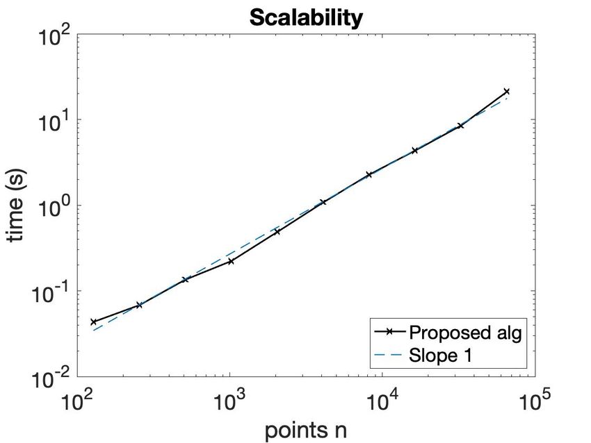
1       Introduction
Multimarginal Optimal Transport (MOT) is the problem of linear programming over joint proba-
bility distributions with fixed marginals, i.e.,

                                         min                      E(X1 ,...,Xk )∼P C(X1 , . . . , Xk )             (1.1)
                                  joint distribution P
                         s.t. i-th marginal of P is µi , ∀i∈[k]

given marginal distributions µ1 , . . . , µk and cost C. Informally, MOT “stitches” together multiple
measurements of a data source in the most likely way. Since data-science problems often require
combining multiple sources of information, MOT arises naturally in applications throughout ma-
chine learning, computer science, and the natural sciences—e.g., information fusion for Bayesian
learning [68, 69], averaging point clouds [2, 34], the n-coupling problem [49, 66], quantile ag-
gregation [53, 65], matching for teams [27, 29, 30], inference from collective dynamics [37, 45],
image processing [61, 67], simulation of incompressible fluids [17, 25], and Density Functional The-
ory [16, 26, 31, 48], among many others.
     However, in most applications, the success of MOT is severely hindered by the lack of efficient
algorithms. Indeed, solving MOT in general requires exponential time in the number of marginals k
and their support sizes n.1 This currently renders most applications intractable beyond tiny input
sizes.
     At first glance, an exponential runtime in n and k may seem unavoidable simply because reading
the input cost C and writing the optimization variable P takes exponential time: they each have
nk exponentially many entries. However, there always exists an optimal solution P of MOT that
is polynomially-sparse (see §2), and in nearly all applications the input cost C has a succinct
representation (e.g., for Wasserstein barycenters, C(x1 , . . . , xk ) = ∑ki,j=1 ∥xi − xj ∥2 is implicit from
the nk locations of the n support points of the k marginal distributions).
     But, of course, just being able to read the input C implicitly in polynomial time and knowing
that there exists a succinctly representable solution P does not mean that one can actually find
such a solution in polynomial time. (See §6 for concrete NP-hard examples.) An obvious barrier is
that the optimization problem (1.1) is over nk exponentially many decision variables. This means
that although MOT is a linear program (LP), standard LP solvers take exponential time if used
out of the box.
     For a very small number of specific MOT problems, there are specially-tailored algorithms that
run in polynomial time—notably, the fluid dynamics MOT problem [14], MOT problems with tree-
structured costs [44], and low-dimensional Wasserstein barycenters [7, 29]. However, it is unknown
if or how these techniques can be extended to the many other MOT problems arising in applications.
     This motivates the central question driving this paper:

                  Are there general “structural properties” that make MOT tractable?

1.1     Contributions
This paper develops a general theory about “structural properties” that render MOT polynomial-
time solvable. We isolate two such properties: decomposability of the cost C into either (i) local
interactions and simple global interactions; or (ii) low-rank interactions and sparse interactions. We
also provide strong evidence that (iii) repulsive costs make MOT intractable by showing that several
such problems of interest are NP-hard to solve—even approximately. These three structures are
    1
    For simplicity, each µi is assumed to have the same support size; differing support sizes is a trivial extension that
changes nothing.

                                                              3
Structure Technique Poly-time algorithm?
Decomposable (§4) Dynamic programming Yes
Low rank (§5) Approximation theory Yes
Repulsive (§6) NP-hardness reductions No
Table 1: The “structural properties” we identify that make MOT tractable/intractable. The struc-
tures are detailed in §1.1, and the algorithmic techniques in §1.2.
quite general, and collectively they encompass many (if not most) of the MOT problems in current
applications.
We highlight that for the tractable structures (i) and (ii), we develop polynomial-time algorithms
with two notable features:
• Sparsity. For both tractable structures (i) and (ii), our algorithms can compute sparse solu-
tions with polynomially many nonzero entries (roughly nk) out of the a priori nk possible2 .
This is in contrast to the popular Sinkhorn algorithm which computes fully dense solutions.
Sparsity enables interpretability, visualization, and efficient downstream computation.
• Exactness. For structure (i), our algorithms can compute exact solutions. Other than our re-
cent specially-tailored algorithm for Wasserstein barycenters [7], these are the first algorithms
for solving MOT problems exactly. (For structure (ii), we solve to arbitrary precision ε and
conjecture NP-hardness of exact solutions; see §5.)
We mention two extensions of our algorithmic results. First, they hold essentially unchanged
for the variant of MOT where some marginals µi are unconstrained (details in Appendix E). This
is helpful in applications with partial observations [37, 43]. Second, our algorithmic results extend
to the entropically-regularized MOT problem (RMOT), which has recently been recognized as an
interesting statistical object in its own right, e.g., [40, 44, 54, 62]. Specifically, we show RMOT is
tractable with either structure (i) or (ii). The only part of our results that do not extend are the
solutions’ sparsity (unavoidable essentially since RMOT solutions are fully dense) and exactness
(unavoidable essentially since RMOT is a convex problem, not an LP).
We now detail the three structures individually; see Table 1 for a summary.
1.1.1 Decomposability structure
In §4, we consider MOT costs C which decompose into a “global interaction” f (x1 , . . . , xk ) between
all variables, and “local interactions” gS (xS ) that depend only on small subsets xS ∶= {xi }i∈S of the
k variables. That is,
C(x1 , . . . , xk ) = f (x1 , . . . , xk ) + ∑ gS (xS ). (1.2)
S∈S
Both interactions must be somehow restricted since in the general case MOT is NP-hard.
We show that MOT is polynomial-time solvable—in fact, exactly and with sparse solutions—
under the following general conditions:
• The global interaction term is “incrementally computable,” meaning essentially that f (x1 , . . . , xk )
can be efficiently computed from reading x1 , . . . , xk once in any order; formal statement in
2
This does not clash with the NP-hardness of computing the sparsest solution for MOT, since we find solutions
that are sparse but not necessarily the sparsest.
4Figure 1: Graphical model G for the decomposable MOT problem in Example 1.1. Vertices corre-
spond to snapshots of the data. Edges exist between snapshots in time windows of length 2.
Definition 4.1. For instance, this includes arbitrary functions of sums of the xi if the xi lie in
a grid, see Example 4.2.
• The local interaction terms can have arbitrary costs gS , so long as the graph G with vertices
{x1 , . . . , xk } and edges {(i, j) ∶ i, j ∈ S for some S} has low treewidth.
Related work to decomposability structure. Several very recent pre-prints [3, 44, 45] study
MOT costs with local interactions and point out an elegant connection to graphical models. Our
work builds upon theirs in several key ways, including (i) their algorithms cannot handle global
interactions, which are crucial for modeling many real-world applications; (ii) for purely local
interactions, they provide provable guarantees in the special case that G is a tree, but otherwise use
heuristics which can converge to incorrect solutions; (iii) our algorithms produce sparse solutions,
whereas theirs produce (succinct representations of) fully dense solutions with exponentially many
nonzero entries; and (iv) our algorithms can solve MOT to machine-precision, whereas theirs are
limited to a few digits of accuracy. See the related work §1.3 for further details.
Applications. This result enables MOT to remain tractable while incorporating complicated
modeling information in the optimization. In some applications, this is critical for avoiding non-
sensical outputs, let alone for achieving good inference. In §4.3, we demonstrate this through the
popular MOT application of inference from collective dynamics [37, 43]. We detail the application’s
premise here since it is an illustrative example of the decomposability structure.
Example 1.1 (Inference from collective dynamics). How can one infer trajectories of indistin-
guishable particles (e.g., cells in a culture, or birds in a flock) given unlabeled measurements µi of
the particle locations at times i ∈ {1, . . . , k} [37, 43]? A joint distribution P as in (1.1) encodes
likelihoods of possible trajectories. To enforce likely trajectories, the cost C(x1 , . . . , xk ) might pe-
nalize local interactions between consecutive pairs xi , xi+1 (e.g., distance traveled) and consecutive
triples xi , xi+1 , xi+2 (e.g., direction changes); see Figure 1. The cost might also incorporate global
interactions, e.g., enforce each cell trajectory to spend a realistic fraction of time in the phases
of some developmental process (e.g., cell cycle, or pathway from progenitor to fully differentiated
cell)—additional information that might be easily measured but previously made the MOT problem
intractable. Previous approaches are unable to reliably handle any of these interactions besides
consecutive pairs (distance traveled), which can lead to inferring nonsensical trajectories; see §4.3.
Our result also provides improved algorithms for MOT problems that are already known to be
tractable. §4.4 demonstrates this for the problem of computing generalized Euler flows—which was
historically the motivation of MOT and has received significant attention, e.g., [14, 16, 22, 23, 24, 25].
While there is a popular, specially-tailored algorithm for this MOT problem that runs in polyno-
mial time [14], it produces solutions that are low-precision (due to poly(1/ε) runtime dependence
on the accuracy ε) and fully dense (with nk nonzero entries), not to mention have numerical pre-
cision issues. In contrast, our algorithm provides exact, sparse solutions. This produces sharp
visualizations whereas the existing algorithm produces blurry ones.
5Extensions. Our algorithms also apply to MOT problems in which we only see partial observa-
tions µi of the hidden states of a graphical model. This is inspired by recent applications of MOT
to particle tracking where the particles’ trajectories evolve via a Hidden Markov Model, and only
partial unlabeled measurements µi of the locations are observed (e.g., from local sensors) [37, 43].
The basic idea is a standard one in estimation and control (e.g., Kalman filtering): augment the
MOT problem by adding for each hidden state a new variable Xi with unconstrained marginal
µi [37, 43]. Since this augmentation does not change the treewidth of the underlying graphical
model, the problem remains tractable if the MOT problem with full measurements is tractable.
This applies, for instance, to arbitrarily complicated stochastic processes so long as their evolutions
depend only on fixed windows of the past (the window size is the treewidth).
In §4.6, we contextualize our decomposability structure with spatial locality structure3 , namely
MOT problems whose cost decomposes spatially as
k
C(x1 , . . . , xk ) = min ∑ c(y, xi ) (1.3)
y∈X i=1
where x1 , . . . , xk are points in some space X , and c ∶ X × X → R is some cost function on X . Such
MOT problems arise in machine learning [2, 34, 68, 69] and economics [27, 29, 30]. We point out
that although this structure can be viewed as decomposability, that requires discretizing the space
which leads to low-precision solutions. In contrast, we show that adapting our recent algorithm
in [7] enables computing exact solutions.
1.1.2 Low rank structure
In §5, we show that MOT can be approximately solved in polynomial time if the cost tensor C
decomposes as a low-rank tensor (given in factored form) plus a sparse tensor (given through
its polynomially many nonzero entries). This lets us handle a wide range of MOT costs with
complex global interactions. These low-rank global interactions are in general different from the
incrementally computable global interactions in our decomposability framework, see Remark 5.1.
It is important to note that the runtime is only polynomial for any fixed rank r. Indeed, we show
in Proposition 5.2 that even without the sparse component of the cost, this is provably unavoidable:
assuming P ≠ N P , there does not exist an algorithm that is jointly polynomial in n, k, and r. This
hardness result extends even to approximate MOT computation.
We remark in passing that the algorithmic techniques we develop also imply a polynomial-time
approximation algorithm for the problem of computing the minimum/maximum entry of a low-rank
tensor given in factored form (Theorem 5.15). We are not aware of any existing algorithms with
sub-exponential runtime. This result may be of independent interest.
Applications. A motivating example is cost functions C(x1 , . . . , xk ) which are sparse polyno-
mials. This is because a sparse polynomial (e.g., a sparse Fourier representation) with r nonzero
coefficients is a rank-r factorization of the tensor containing the values of C.
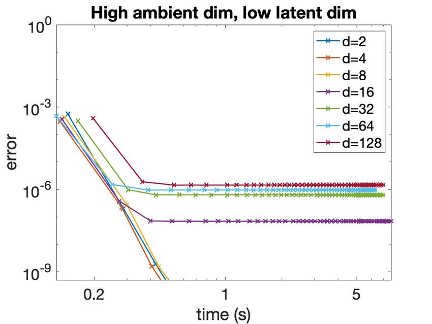
In §5.3 we consider another application: the Wasserstein barycenter problem with multimarginal
entropic regularization. This regularization is different from the popular pairwise regularization [14]
and is motivated by its statistical and computational properties [37, 44]; details in §5.3. We target
this problem specifically in the regime that the number of points n is very large and the number
of marginals k is fixed, which is motivated by large-scale machine learning applications. In this
3
[29] calls this structure “localization”, and [58] calls it “infimal convolution”; we use the term “spatial locality”
instead to distinguish it from other local interactions (e.g., temporally-local interactions as in Example 1.1).
6regime, nk is intractable even if k is a small constant. Since the Wasserstein barycenter cost
admits a low-rank decomposition, our techniques yield an algorithm that scales near-linearly in
n and reasonably well in ε. Further, this algorithm can scale to high-dimensional problems with
latent low-dimensional structure—a common occurence in real-world machine learning datasets.
This is the first algorithm for this problem that scales in n better than nk while also scaling
sub-exponentially in the ambient dimension d.
1.1.3 Repulsive structure
In contrast to the tractability results for the above two structures, §6 turns to intractability results.
We isolate “repulsive costs” as a source of intractability. Informally, these are costs C(x1 , . . . , xk )
which encourage diversity between x1 , . . . , xk ; we refer the reader to the nice survey [35] for a
detailed discussion of such MOT problems and their many applications.
We provide strong evidence that repulsive costs lead to intractable MOT problems by proving
that several such MOT problems of interest are NP-hard not only to solve, but even to approxi-
mate. In §6.2 we show this for MOT with determinant cost, and in §6.3 we show this for Density
Functional Theory with Coulomb-Buckingham potential. Additionally, in §6.4, we observe that the
classical problem of evaluating the convex envelope of discrete function is an instance of MOT, and
leverage this connection to show that MOT is NP-hard to approximate with supermodular costs, yet
tractable with submodular costs. This dichotomy provides further evidence for the intractability
of repulsive costs, since the intractable former problem is “repulsive”, whereas the tractable latter
problem is “attractive”.
To the best of our knowledge, these are the first results that rigorously demonstrate intractability
of MOT with repulsive costs. This is a first step towards explaining why—despite a rapidly growing
literature—there has been a lack of progress in developing polynomial-time algorithms with provable
guarantees for many MOT problems with repulsive costs.
1.2 Techniques
We begin in §3 by viewing the MOT problem from the perspective of implicit, exponential-size
LP. We consider three algorithms for this problem whose exponential runtime can be isolated
into a single bottleneck—and thus can be implemented in polynomial-time whenever that bot-
tleneck can. These algorithms are the Ellipsoid algorithm ELLIPSOID [42, 47], the Multiplicative
Weights algorithm MWU [77], and the natural multidimensional analog of Sinkhorn’s scaling algo-
rithm SINKHORN [14, 59]. The first two are classical algorithms for general implicit LP, but do
not appear in the MOT literature; whereas the third is specially tailored to the MOT and RMOT
problems and is currently the predominant approach for them (see §1.3).
The bottlenecks of these three algorithms are shown to be natural analogs of the membership
oracle for the feasible set of the dual LP of MOT. Namely, given weights p1 , . . . , pk ∈ Rn , compute
k
min Cj1 ,...,jk − ∑[pi ]ji (1.4)
(j1 ,...,jk )∈[n]k i=1
either exactly (for ELLIPSOID), approximately (for MWU), or with the “min” replaced by a “softmin”
(for SINKHORN). We call these three tasks the MIN, AMIN, and SMIN oracles, respectively.
This oracle abstraction is helpful for showing that a class of MOT problems is either tractable or
intractable. From an algorithmic perspective, the oracle abstraction reduces solving an MOT prob-
lem in polynomial time to solving any of these three oracles in polynomial time—which are phrased
as more standard combinatorial-optimization problems, and thus are more directly amenable to
7Algorithm Oracle Runtime Exact? Sparse?
ELLIPSOID MIN Theorem 3.5 Yes Yes
MWU AMIN Theorem 3.7 No Yes
SINKHORN SMIN Theorem 3.10 No No
Table 2: These MOT algorithms have polynomial runtime except for a single bottleneck (“oracle”).
The number of oracle computations is poly(n, k) for ELLIPSOID, poly(n, k, Cmax /ε) for MWU, and
log n ⋅ poly(k, Cmax /ε) for SINKHORN. For the latter two algorithms, these polynomials are quite
small. For the RMOT problem, only SINKHORN applies.
standard algorithmic techniques. From the hardness perspective, we show that this reduction from
MOT to the oracles is at no loss of generality since the opposite reduction also holds4 , and thus in
order to prove NP-hardness of MOT it suffices to show NP-hardness of the oracles.
Two remarks. 1) These algorithms have important tradeoffs: ELLIPSOID is strongly polynomial
(i.e., can solve exactly or to high-precision), ELLIPSOID and MWU find sparse solutions, MWU and
SINKHORN can have numerical precision issues when solving past a couple digits of accuracy, and
SINKHORN is the most scalable in n. We emphasize that while MWU and SINKHORN are practical,
ELLIPSOID is not—our use of ELLIPSOID is intended solely as a proof of concept that MOT can be
solved in strongly polynomial time, see Remark 3.6. 2) Expressing the “marginalization” bottleneck
of SINKHORN equivalently as this SMIN oracle puts SINKHORN on equal footing with the other two
classical algorithms in terms of their reliance on separation oracle variants, see Remark 3.2.
1.2.1 Exploiting decomposability structure
Consider the setting where C is decomposed into a sum of short-range interaction terms and one
simple global interaction term. The short-range interaction terms can be viewed as corresponding to
the factors of a graphical model of constant treewidth. Therefore, if there were no global interaction
term, we could implement MIN and SMIN in polynomial time using the standard max-plus and sum-
product algorithms on a constant-width junction tree for the graphical model. We show how to
augment the max-plus and sum-product algorithms to handle the global interaction term. This
enables the polynomial-time implementation of ELLIPSOID (via MIN), SINKHORN (via SMIN), and
MWU (since AMIN can be simulated by SMIN). Details in §4.
1.2.2 Exploiting low rank structure
Here, the three variants of the MIN oracle amount to (approximately) computing the minimum entry
of a low-rank tensor C which has been perturbed by weights as described in (1.4). We show how
to approximate the SMIN oracle in polynomial time, which also implies an efficient implementation
of the AMIN oracle. This task amounts to computing
1
− log ∑ [ exp ((d1 ⊗ ⋯ ⊗ dk ) ⊙ K)] (1.5)
η (j1 ,...,j )∈[n]k
j1 ,...,jk
k
where K ∶= exp[−ηC] is the entrywise exponentiated “Gibbs kernel” corresponding to the cost C,
di ∶= exp[−ηpi ] are scalings formed by entrywise exponentiating the oracle weights, and η is the
softmin parameter.
4
This is inspired by, but different from, the classical relations between strong membership and strong optimization
oracles for general LP [42]. See Remark 6.4 for details.
8A basic fact we leverage is that if a tensor has a known low-rank factorization, then the sum
of its exponentially many entries can be computed in polynomial time. The relevance is that if K
has a known low-rank factorization, then so does the “diagonally scaled” tensor (d1 ⊗ ⋯ ⊗ dk ) ⊙ K,
and thus we can compute (1.5) efficiently.
However, a key obstacle is that if C is low-rank, then the corresponding Gibbs kernel K =
exp[−ηC] is in general not low-rank. We overcome this by proving that K is approximately low-
rank, and moreover that we can efficiently compute an approximate low-rank factorization. This
is done by approximating the exponential function c ↦ exp(−ηc) by a low-degree polynomial p(c),
defining K̃ = p[C] where the polynomial is applied entrywise, and exploiting the fact that a low-
degree polynomial applied entrywise to a low-rank tensor is a low-rank tensor (whose low-rank
factorization is moreover efficiently computable). Details in §5.
1.2.3 Hardness for repulsive structure
Our main insight is that approximating MOT and implementing an AMIN oracle are polynomial-
time equivalent. We emphasize that this result holds for any MOT cost and thus may be helpful for
proving future hardness results for other MOT problems. Operationally, this equivalence reduces
proving the inapproximability of MOT to proving the NP-hardness of the associated AMIN oracle
problem. This is often simpler because the AMIN oracle problem is formulated in a more standard
way for combinatorial optimization. In fact, in all MOT problems with repulsive costs considered
in §6, it is NP-hard even to approximately solve the AMIN problem in the special case that all
weights are zero—i.e., it is NP-hard even to approximate the minimum entry of the cost tensor C.
We briefly mention the technical tools that go into proving the reduction from AMIN to approx-
imating MOT, which is the relevant direction for proving hardness of MOT. The proof leverages
recent developments on zero-th order optimization of approximately convex functions [13, 63]. This
connection is based on an exact convex relaxation that equivalently recasts the discrete optimization
problem defining AMIN as a convex optimization problem whose objective can be approximately
evaluated by approximately solving an auxiliary MOT problem. Details in §6.
1.3 Related work
Sinkhorn scaling. Currently, the predominant algorithmic approach for MOT is to solve an
entropically regularized version of it with SINKHORN, (a.k.a. Iterative Proportional Fitting or It-
erative Bregman Projections or RAS algorithm), see e.g., [14, 15, 16, 17, 44, 45, 55, 59] among
many others. SINKHORN has long been known to converge (see the survey [46] for a historical
perspective), and recent work has proven that a small number of iterations suffice [39, 52, 73].
This line of work is orthogonal—in fact, complementary—to the present paper which shows how
to efficiently implement the individual iterations for structured costs (in general, each iteration
takes exponential time). Our main results provide general conditions under which SINKHORN (and
other algorithms) can efficiently solve MOT—this recovers all known special cases where SINKHORN
is efficiently implementable, and furthemore identifies broad new families of MOT problems where
this is possible.
Connections to graphical models. Connections between graphical models and optimization
over marginal polytopes date back at least to [71, 75], and have been nicely fleshed out for the
specific case of MOT in the very recent pre-prints [3, 45]. It is implicit from this connection that
one can use the junction tree algorithm from the graphical models literature (e.g., [50]) to effi-
ciently implement SINKHORN for MOT costs that decompose purely into local interactions whose
9corresponding graphical model has bounded treewidth. This is the starting point of our decompos-
ability structure. However, our result improves on this in several key ways, the most salient being:
we show how to augment the junction tree algorithm to incorporate global interactions; and we
provide alternative algorithms to SINKHORN that—in contrast—produce solutions that are exact,
sparse, and do not suffer from numerical precision issues.
Optimization over joint distributions. Optimization problems over exponential-size joint dis-
tributions appear in many domains. For instance, they arise in game theory when computing cor-
related equilibria (e.g., [57]); however, in that case the optimization has different constraints which
lead to different algorithms. Such problems also arise in variational inference (e.g., [75]); however,
the optimization there typically constrains this distribution to ensure tractability (e.g., mean-field
approximation restricts to product distributions).
2 Preliminaries
General notation. The set {1, . . . , n} is denoted by [n], and the simplex {µ ∈ Rn⩾0 ∶ ∑ni=1 µi = 1}
is denoted by ∆n . The notation Õ suppresses polylogarithmic factors in n, k, Cmax , ε, and η.
Throughout, we assume for simplicity of exposition that all entries of the input C and µ1 , . . . , µk
have bit complexity at most poly(n, k); the general case is a straightforward extension.
Tensor notation. In the introduction, the entries of the cost tensor C are denoted by the intuitive
notation C(x1 , . . . , xk ); for the algorithmic development in the sequel, we adopt the mathematically
convenient notation Cj1 ,...,jk . The k-fold product space Rn ⊗ ⋯ ⊗ Rn is denoted by (Rn )⊗k , and
similarly for (Rn⩾0 )⊗k . Let P ∈ (Rn )⊗k . Its i-th marginal, i ∈ [k], is denoted by mi (P ) ∈ Rn and has
entries [mi (P )]j ∶= ∑j1 ,...,ji−1 ,ji+1 ,...,jk Pj1 ,...,ji−1 ,j,ji+1 ,...,jk . For shorthand, we often denote an index
(j1 , . . . , jk ) by ⃗j. The sum of P ’s entries is denoted by m(P ) = ∑⃗j P⃗j . The maximum absolute value
of P ’s entries is denoted by ∥P ∥max ∶= max⃗j ∣P⃗j ∣, or simply Pmax for short. The operations ⊙ and
⊗ respectively denote the entrywise product and the Kronecker product. A non-standard notation
we use throughout is that f [P ] denotes a function f ∶ R → R (typically exp, log, or a polynomial)
applied entrywise to a tensor P .
2.1 Multimarginal Optimal Transport
The transportation polytope between measures µ1 , . . . , µk ∈ ∆n is
M(µ1 , . . . , µk ) ∶= {P ∈ (Rn⩾0 )⊗k ∶ mi (P ) = µi , ∀i ∈ [k]} . (2.1)
In this notation, the MOT problem (1.1) for cost C ∈ (Rn )⊗k and measures µ1 , . . . , µk ∈ ∆n is the
LP
min ⟨P, C⟩. (MOT)
P ∈M(µ1 ,...,µk )
In the k = 2 matrix case, (MOT) is the standard Kantorovich formulation of OT [74]. Its dual LP
is
k k
k
max ∑⟨pi , µi ⟩ subject to Cj1 ,...,jk − ∑[pi ]ji ⩾ 0, ∀(j1 , . . . , jk ) ∈ [n] . (MOT-D)
p1 ,...,pk ∈R i=1
n
i=1
10A basic, folklore fact about MOT is that it always admits a sparse optimal solution. Indeed,
since MOT is an LP in standard form it has an optimal solution at some vertex of M(µ1 , . . . , µk )—
and vertices of M(µ1 , . . . , µk ) have sparsity at most nk −k +1 since there are nk equality constraints
defining M(µ1 , . . . , µk ), and at least k − 1 of these are linearly dependent.
Lemma 2.1 (Sparse solutions for MOT). For any cost C ∈ (Rn )⊗k and any marginals µ1 , . . . , µk ∈
∆n , there exists an optimal solution P to MOT that has at most nk − k + 1 nonzero entries.
Definition 2.2 (ε-approximate MOT solution). P is an ε-approximate MOT solution if P is feasible
(i.e., P ∈ M(µ1 , . . . , µk )) and ⟨C, P ⟩ is at most ε more than the optimal value.
2.2 Regularization
We introduce two standard regularization operators. First is the Shannon entropy H(P ) ∶=
− ∑⃗j P⃗j log P⃗j of a tensor P ∈ (Rn⩾0 )⊗k with entries summing to m(P ) = 1. Second is the soft-
min operator, which is defined for parameter η as
m
1
sminη ai ∶= − log (∑ e−ηai ) . (2.2)
i∈[m] η i=1
We make use of the following elementary bound, which bounds the pointwise error between the
min and smin operators based on the regularization and the number of points.
Lemma 2.3 (Softmin approximation bound). For any a1 , . . . , am ∈ R and η > 0,
log m
min ai − ⩽ sminη ai ⩽ min ai .
i∈[m] η i∈[m] i∈[m]
The entropically regularized MOT problem (RMOT for short) is the convex optimization problem
min ⟨P, C⟩ − η −1 H(P ). (RMOT)
P ∈M(µ1 ,...,µk )
This is the natural multidimensional analog of entropically regularized OT, which has a rich litera-
ture in statistics [51] and transportation theory [76], and has recently attracted significant interest
in machine learning [33, 59]. The convex dual of (RMOT) is the convex optimization problem
k k
max ∑⟨pi , µi ⟩ + sminη (Cj1 ,...,jk − ∑[pi ]ji ) . (RMOT-D)
p1 ,...,pk ∈R i=1
n
(j1 ,...,jk )∈[n]k i=1
In contrast to MOT, there is no analog of Lemma 2.1 for RMOT: the unique optimal solution
to RMOT is dense. Further, this solution may not even be “approximately” sparse.
We define P to be an ε-approximate RMOT solution in the analogous way as in Definition 2.2.
A basic, folklore fact about RMOT is that if the regularization η is sufficiently large, then RMOT
and MOT are equivalent in terms of approximate solutions.
Lemma 2.4 (MOT and RMOT are close for large regularization η). Let P ∈ M(µ1 , . . . , µk ), ε > 0,
and η ⩾ ε−1 k log n. If P is a ε-approximate RMOT solution, then P is also a (2ε)-approximate
MOT solution; and vice versa.
Proof. Since a discrete distribution supported on nk atoms has entropy at most k log n [32], the
objectives of MOT and RMOT differ pointwise by at most η −1 k log n ⩽ ε. Since MOT and RMOT
also have the same feasible sets, their optimal values therefore differ by at most ε.
113 Oracles and algorithms
In this section, we consider three algorithms for MOT (the last of which also applies to RMOT).
Each algorithm is iterative and requires only polynomially many iterations. The key issue for each
algorithm is the per-iteration runtime, which is in general exponential (roughly nk ). We isolate the
respective bottlenecks of these three algorithms into what we call the min oracle MIN, approximate
min oracle AMIN, and softmin oracle SMIN.
Definition 3.1 (Oracles). Consider weights p = (p1 , . . . , pk ) ∈ Rn×k , approximation accuracy ε > 0,
and regularization parameter η > 0.
• MIN(p) returns min(j1 ,...,jk )∈[n]k Cj1 ,...,jk − ∑ki=1 [pi ]ji .
• AMIN(p, ε) returns min(j1 ,...,jk )∈[n]k Cj1 ,...,jk − ∑ki=1 [pi ]ji up to additive error ε.
k
• SMIN(p, η) returns sminη Cj1 ,...,jk − ∑[pi ]ji .
(j1 ,...,jk )∈[n]k i=1
Remark 3.2 (Value vs tuple, a.k.a., membership vs separation). The MIN and AMIN oracles re-
turn only the (approximately) minimizing value; one can analogously define ARGMIN and ARGAMIN
oracles which return an (aproximately) minimizing tuple. The MIN and AMIN are essentially (ap-
proximate) membership oracles for the feasible set of the dual LP (MOT-D), whereas ARGMIN and
ARGAMIN oracles are (approximate) separation oracles. For general LP, membership and separa-
tion oracles are not equivalent [42]. However, for the special case of MOT, we show that there is no
difference: MIN and ARGMIN are polynomial-time equivalent, and same for AMIN and ARGAMIN;
proof in Appendix A.1.
Remark 3.3 (AMIN as special case of SMIN). By Lemma 2.3, the AMIN(p, ε) oracle is imple-
mentable by the SMIN(p, η) oracle with regularization η ⩾ ε−1 k log n. Thus by Remark 3.2, the
SMIN oracle is essentially a specific type of approximate membership oracle for (MOT-D).
Remark 3.4 (Interpretations as inference problems). The MIN, AMIN, and SMIN oracles have
equivalent interpretations from the perspective of statistical physics. Consider a random variable
J = (J1 , . . . , Jk ) ∈ [n]k distributed according to the Gibbs measure
k
1
P(J = (j1 , . . . , jk )) = exp (−η (Cj1 ,...,jk − ∑[pi ]ji )) . (3.1)
Z(p, η) i=1
The MIN (AMIN) oracle computes the Maximum Likelihood Estimate (approximately). The SMIN
oracle computes the log-partition function log(Z(p, η)).
In the following three subsections, we describe the three MOT algorithms and provide polyno-
mial runtime guarantees for them conditional on an efficient implementation of their corresponding
bottleneck oracle. See Table 2 for a summary of this section.
3.1 MIN oracle and the Ellipsoid algorithm
Among the most classical LP algorithms is the Ellipsoid algorithm ELLIPSOID [47]. A key feature
of ELLIPSOID is that it can be implemented in polynomial time for an LP with exponentially
many constraints so long as it has polynomially many variables and the corresponding separation
oracle is polynomial-time computable [41, 42]. Although this result does not immediately apply
12to MOT as it has exponentially many variables, it can apply to its dual (MOT-D) since that has
only polynomially many variables. This enables one to compute an optimal dual solution whenever
the separation oracle for (MOT-D)—which can be implemented using MIN (see Remark 3.2)—is
efficiently computable. While an optimal dual solution in general does not “help” to find an optimal
primal solution [18, Exercise 4.17], the following result shows that in the special case of MOT it
does—and moreover one can use it to find a sparse primal solution. This result is [7, Proposition
3.2] and is summarized as follows.
Theorem 3.5 (ELLIPSOID). An optimal vertex solution for (MOT) can be found using poly(n, k)
calls to the MIN oracle and poly(n, k) additional time. The solution is returned as a sparse tensor
with at most nk − k + 1 nonzero entries.
Remark 3.6 (Practical alternative). We use ELLIPSOID solely as a proof of concept that problems
are tractable. Developing more practical polynomial-time algorithms is an interesting, problem-
specific direction for future work. In practice, we use column generation (see e.g., [18, Chapter
6]) rather than ELLIPSOID since this has better empirical performance yet still has the same MIN
bottleneck, solves MOT exactly, and produces sparse solutions.
3.2 AMIN oracle and the Multiplicative Weights algorithm
The other classical algorithm for solving exponential-size LP with implicit structure is the Mul-
tiplicative Weights Update algorithm MWU [77, 78]. While MWU is designed specifically for positive
LPs, MOT can reduced to such a problem by appropriately generalizing the recent use of MWU in the
k = 2 matrix case of Optimal Transport in [20, 60]. As we show in the following result, the further
“structure” that MWU needs to solve MOT is efficient approximate computation of the membership
oracle for the dual (MOT-D)—namely, efficient computation of AMIN. For brevity, pseudocode and
proof details are deferred to Appendix A.2.
Theorem 3.7 (MWU). For any ε > 0, an ε-approximate solution to (MOT) can be found using
poly(n, k, Cmax /ε) calls to the AMIN oracle with accuracy Θ(ε), and poly(n, k, Cmax /ε) additional
time. The solution is returned as a sparse tensor with poly(n, k, Cmax /ε) nonzero entries.
3.3 SMIN oracle and the Sinkhorn algorithm
The Sinkhorn algorithm SINKHORN is specifically tailored to MOT and RMOT, and does not ap-
ply to general exponential-size LP. Unlike ELLIPSOID and MWU, SINKHORN is popular in the MOT
community (see §1.3). Yet this algorithm is less understood from the perspective of implicit,
exponential-size LP, and as such we briefly introduce the algorithm to add insight into its specific
bottleneck. Further details and pseudocode for SINKHORN are provided in Appendix A.3.
SINKHORN solves RMOT, and thus also MOT for sufficiently high regularization η (Lemma 2.4).
SINKHORN is based on the first-order optimality conditions of RMOT: the unique solution is the
unique tensor in M(µ1 , . . . , µk ) of the form P = (d1 ⊗ ⋯ ⊗ dk ) ⊙ K, where K = exp[−ηC] is the en-
trywise exponentiated “Gibbs kernel”, and d1 , . . . , dk ∈ Rn>0 are positive vectors. SINKHORN computes
such a solution by initializing all di to 1 (no scaling), and then iteratively updating some di so that
the i-th marginal mi (P ) of the current scaled iterate P is µi . Although correcting one marginal
can detrimentally affect other marginals, SINKHORN nevertheless converges—in fact, rapidly so.
However, each iteration requires the following bottleneck, which in general takes exponential time.
Definition 3.8 (MARG). Given regularization η > 0, scalings d ∶= (d1 , . . . , dk ) ∈ Rn×k
>0 , and index
i ∈ [k], the marginalization oracle MARG(d, η, i) returns mi ((d1 ⊗ ⋯ ⊗ dk ) ⊙ K).
13Conditional on this bottleneck MARG being efficiently computable, SINKHORN is efficient due to
known bounds on its iteration complexity [52].5 To obtain a final feasible solution, the approxi-
mately feasible point computed by SINKHORN is post-processed via a simple rounding algorithm (it
adjusts the scalings and adds a rank-one term). Importantly, this rounding has the same MARG
bottleneck. Details in Appendix A.3. The runtime guarantees are summarized as follows.
Theorem 3.9 (SINKHORN for RMOT). For any accuracy ε > 0 and regularization η > 0, an ε-
approximate solution to RMOT can be found using T calls to the MARG oracle and O(nT ) additional
time, where T = Õ(poly(k, η, Cmax , 1/ε)). The solution is of the form
P ∶= (⊗kj=1 dj ) ⊙ exp[−ηC] + (⊗kj=1 vk ) (3.2)
and is output implicitly via the vectors d1 , . . . , dk ∈ Rn>0 and v1 , . . . , vk ∈ Rn⩾0 .
Theorem 3.10 (SINKHORN for MOT). For any accuracy ε > 0, an ε-approximate solution to
MOT can be found using T calls to the MARG oracle and O(nT ) additional time, where T =
Õ(poly(k, Cmax /ε)). The solution is outputted as in Theorem 3.9.
Note that the number of MARG calls—i.e., the number of SINKHORN iterations—depends on n
only logarithmically. This makes SINKHORN particularly scalable.
We conclude this discussion by pointing out the polynomial-time equivalence of the MARG and
SMIN oracles. In light of Theorem 3.10, this puts SINKHORN on “equal footing” with the classical
algorithms ELLIPSOID and MWU in terms of their reliances on related membership oracles.
Lemma 3.11 (Equivalence of MARG and SMIN). Each of the oracles MARG and SMIN can be
implemented using poly(n) calls of the other oracle and poly(n, k) additional time.
It is obvious that SMIN can be implemented with a single MARG call (add up the answer). The
converse is more involved and requires n calls; the proof is deferred to Appendix A.1.
4 Exploiting decomposable structure
In this section we consider MOT problems with cost tensors C that decompose into a “global
interaction” f ∶ [n]k → R that depends on all k variables, and “local interactions” gS ∶ [n]S → R
that depend only on small subsets ⃗jS ∶= {ji }i∈S of the k variables. That is,
C⃗j = f (⃗j) + ∑ gS (⃗jS ), ∀⃗j ∶= (j1 , . . . , jk ) ∈ [n]k . (4.1)
S∈S
Both interactions must be somehow restricted since in the general case MOT is NP-hard (see §4.1).
The main result of this section is that tractability is in fact ensured for a broad class of global and
local interactions (Theorem 4.6).
The section is organized as follows. §4.1 formally defines the structure required for the interac-
tions. §4.2 provides polynomial-time algorithms for these MOT problems. §4.3 and §4.4 demonstrate
our result in the applications of particle tracking and generalized Euler flows, respectively. The
former application shows how our result enables incorporating complicated information in MOT.
The latter application shows how our result also provides improved solutions for MOT problems
that are already known to be tractable. Finally, §4.5 mentions an extension to partial observations;
and §4.6 points out that although spatially-local costs can be viewed as decomposable costs, this
is not always the best approach.
5
To be precise, the iteration-complexity bounds in the literature are written for MOT. Extending to RMOT
requires a more careful bound of the entropy regularization term since it is nonnegligible in this case. However, this
is easily handled using the techniques of [5]; details in Appendix A.3.
144.1 Interactions
4.1.1 Global interactions
Clearly the global interaction f must be somehow restricted, since otherwise any cost C is trivially
expressable via (4.1) with C = f , and this general case is NP-hard. We show tractability for the
following broad class of global interactions f . These are essentially the functions which can be
“incrementally computed” by reading the variables j1 , . . . , jk once in any order, either sequentially
or by combining batches, while always maintaining a small “state”. This state is formalized by a
sufficient statistic hS (⃗jS ) of the variables ⃗jS for computing f (⃗j).
Definition 4.1 (Incrementally-computable global interactions). A function f ∶ [n]k → R is said to
be incrementally computable if there exists some set Ω of poly(n, k) cardinality and some functions
hS ∶ [n]S → Ω for each S ⊂ [k] such that
• Initial computation. For any i ∈ [k], we can compute h{i} (ji ) in poly(n, k) time given ji .
• Incremental computation. For any disjoint A, B ⊆ [k], we can compute hA∪B (⃗jA∪B ) in poly(n, k)
time given hA (⃗jA ) and hB (⃗jB ).
• Final computation. f = φ ○ h[k] for a function φ ∶ Ω → R we can compute in poly(n, k) time.
Two remarks. First, if Definition 4.1 did not constrain ∣Ω∣, then every efficiently computable
function f ∶ [n]k → R would trivially satisfy it with Ω = [n]k . In words, a small number of states ∣Ω∣
means that f depends on the individual variables through a “concise” summary statistic. Our final
runtime for solving MOT depends polynomially on ∣Ω∣. Second, Definition 4.1 is not completely
rigorous as written because in order to write “poly(n, k)” bounds, one must technically consider a
family of functions {fn,k }n,k . However, we avoid this notational overhead since every f we consider
naturally belongs to a family and thus the meaning of this abuse of notation is clear.
Example 4.2 (Functions of the sum). Several popular MOT problems have costs of the form
k
Cj1 ,...,jk = φ (∑ xi,ji ) , (4.2)
i=1
for some function φ, where xi,j ∈ Rd is the j-th point in the support of marginal µi , see e.g.,
the surveys [35, 58]. This is an incrementally computable global interaction if the points xi,j lie
on some uniform grid G in Rd in constant dimension d. Indeed, Definition 4.1 is satisfied for
f (x1 , . . . , xk ) = φ(∑ki=1 xi ) with hS (xS ) ∶= ∑i∈S xi and Ω = ∪ki=1 Gi , where Gi denotes the Minkowski
sumset of i copies of G. Crucially, the fact that G is a grid in constant dimension ensures that
∣Gi ∣ ⩽ id ∣Gi ∣ = poly(i) ⋅ ∣G∣, and thus ∣Ω∣ = poly(k) ⋅ ∣G∣. This generalizes in the obvious way to other
sets with additive combinatorial structure. Therefore our polynomial-time algorithm for solving
problems with global interactions (Theorem 4.6) computes exact, sparse solutions for MOT problems
with this structure, including:
• Quantile aggregation, in which case φ(t) = 1[t ⩽ q] or φ(t) = 1[t ⩾ q] for some input quantile
q, and d = 1; see e.g., the references within the recent paper [21].
• MOT with repulsive harmonic cost, in which case φ(t) = ∥t∥2 [35].
• Wasserstein barycenters [2], a.k.a. the n-coupling problem [66], in which case φ(t) = −∥t∥2 .6
6
Note this example can also be solved with specially tailored algorithms, namely the one in [7], or the LP refor-
mulation in [34] which is exact for fixed support Ω = Gk in the special case of uniform grids.
154.1.2 Local interactions
The local interactions {gS }S∈S must also be somehow restricted, since otherwise MOT can encode
NP-hard problems such as finding a maximum clique in a graph (see Appendix C.1) or computing
the max-cut of a graph (when the local interactions correspond to an Ising model). An underlying
source of difficulty in both these cases is that there are interactions between essentially all pairs of
variables. This difficulty is isolated formally in the following definition. Note that the graphical
model is defined only through the sets S of locally interacting variables (a.k.a. factors in the
graphical models jargon), and is otherwise independent of the interaction functions gS .
Definition 4.3 (Graphical model for local interactions). Let S be a collection of subsets of [k].
The graphical model structure corresponding to S is the undirected graph GS = (V, E) with vertices
V = [k] and edges E = {(i, j) ∶ i, j ∈ S for some S ∈ S}.
We show tractability for a broad family of local interactions: the functions {gS }S∈S can be
arbitrary so long as the corresponding graphical model structure GS has low treewidth. While the
runtimes of our algorithms depend exponentially on the treewidth, we emphasize that in nearly all
current real-world applications of MOT falling under this decomposability framework, the treewidth
is a very small constant (typically under 3, say).
The concept of treewidth is based on the concept of a junction tree; both are standard in the
field of graphical models. We briefly recall the definitions; for further background see, e.g., [19, 50].
Definition 4.4 (Junction tree). A junction tree T = (VT , ET , {Bu }u∈VT ) for a graph GS = (V, E)
consists of a tree (VT , ET ) and a set of bags {Bu ⊆ V }u∈VT satisfying:
• For each variable i ∈ V , the set of nodes Ui = {u ∈ VT ∶ i ∈ Bu } induces a subtree of T .
• For each edge e ∈ E, there is some bag Bu containing both endpoints of e.
The width of the junction tree is one less than the size of the largest bag: width(T ) = maxu∈VT ∣Bu ∣−1.
Definition 4.5 (Treewidth). The treewidth of a graph is the width of its minimum-width junction
tree.
4.2 Algorithms
We are now ready to state the main result of this section.
Theorem 4.6 (Solving MOT for decomposable costs). Consider costs C ∈ (Rn )⊗k which decompose
as in (4.1) into an incrementally-computable global interaction f and poly(n, k) local interactions
{gS }S∈S whose corresponding graphical model structure GS has treewidth w. For any fixed w, an
optimal vertex solution to MOT can be computed in O(poly(n, k)) time. The solution is returned
as a sparse tensor with at most nk − k + 1 nonzero entries.
Theorem 4.7 (Solving RMOT for decomposable costs). Consider the setup in Theorem 4.6. For
any fixed treewidth w and accuracy ε > 0, an ε-approximate solution to RMOT can be computed in
poly(n, k, Cmax , 1/ε, η) time. The solution is returned as in Theorem 3.9.
By Theorem 3.5, in order to prove Theorem 4.6 it suffices to show that the corresponding MIN
oracle can be implemented in polynomial time. Similarly, by Theorem 3.9 and Lemma 3.11, in order
to prove Theorem 4.7 it suffices to show that the corresponding SMIN oracle can be implemented
in polynomial time. Both oracles are efficiently implemented in the following lemma.
16Algorithm 1 Dynamic programming for decomposable structure (details in proof of Lemma 4.8)
Input: Incrementally-computable global interaction f , local interactions {gS }S∈S , weights p ∈ Rnk
Output: Values of MIN(p) and SMIN(p, η) oracles
1: Compute junction tree T = (VT , ET , {Bv }) for graphical model GS .
2: Compute “augmented” junction tree T ′ = (VT , ET , {Bv′ }) from T .
3: Construct “augmented” graphical model P′ corresponding to junction tree T ′ .
4: Compute MLE and partition function for P′ using junction tree T ′ [50, Chapter 10].
5: Compute MIN(p) from MLE, and SMIN(p, η) from partition function.
Lemma 4.8 (Efficient oracles for decomposable costs). Consider the setup in Theorem 4.6. The
MIN and SMIN oracles can be implemented in poly(n, k) time.
Proof. Recall from Remark 3.4 that computing the MIN (resp., SMIN) oracle is equivalent to com-
puting the MLE (resp., posterior) of the Gibbs distribution
k
1
P(J⃗ = ⃗j) = exp(−ηf (⃗j)) ∏ exp(−ηgS (⃗jS )) ∏ exp(η[pi ]ji ). (4.3)
Z(p, η) S∈S i=1
Note that the potentials exp(η[pi ]ji ) do not affect the graphical model structure since they are
single-variable functions. Thus, if there were no global interaction f , the Gibbs distribution would
be given by a graphical model with structure GS , in which case the MLE and Posterior could be
computed by a standard junction tree algorithm in poly(n, k) time as in e.g., [50, Chapter 10]
because GS has constant treewidth w.
We handle the global interaction f by adding auxiliary variables corresponding to its incrementally-
computable structure—while still maintaining low treewidth. Pseudocode is provided in Algo-
rithm 1; we detail the main steps below. See also Figure 2 for an illustrated example. In what
follows, let hS and φ be as in Definition 4.1.
1. Compute a width-w junction tree T = (VT , ET , {Bu }u∈VT ) for GS . Choose a root ρ ∈ VT
and adjust T so that each non-leaf-node has exactly two children, and also so that for each
variable i ∈ [k] there is a leaf l(i) ∈ VT whose bag Bl(i) is the singleton set containing Ji .
2. Define an “augmented” junction tree T ′ = (VT , ET , {Bu′ }u∈VT ) with the same graph structure,
but with up to three extra variables in each bag: set Bu′ = Bu ∪ {Hu }, and additionally add
Hw to Bu′ for any children w of u.
Note that T ′ is a junction tree for the “augmented” graph G′ = (V ′ , E ′ ) where V ′ = V ∪
{Hu }u∈VT and E ′ = E ∪ {{Hu , Hw } ∶ u, w ∈ VT , w is child of u} ∪ {{Hl(i) , Ji } ∶ i ∈ [k]}.
3. Define an “augmented” graphical model P′ with structure G′ over variables J⃗ and H ⃗ for which
J⃗ has marginal distribution P and H ⃗ is a deterministic function of J.⃗ For this it is helpful to
introduce some notation. For u ∈ VT , let Au = {i ∈ [k] ∶ l(i) in subtree of T rooted at u}. For
disjoint A, A′ ⊂ [k], let rA,A′ denote the polynomial-time computable function in Definition 4.1
for which hA∪A′ (⃗jA∪A′ ) = rA,A′ (hA (⃗jA ), hA′ (⃗jA′ )). We say that ⃗j and h
⃗ are consistent with
respect to T if: hl(i) = h{i} (ji ) for all i ∈ [k], hu = h∅ for all leaves u ∈ VT ∖ l−1 ([k]), and
′
hu = rAw1 ,Aw2 (hw1 , hw2 ) for all u ∈ VT with children w1 and w2 . Now define P′ by
k
1
P′ (J⃗ = ⃗j, H ⃗ =
⃗ = h) exp(−ηφ(h ρ )) ∏ exp(−ηgS (⃗jS )) ∏ exp(η[pi ]ji ). (4.4)
Z ′ (p, η) S∈S i=1
17(a) Junction tree. (b) Augmented junction tree.
Figure 2: Example of how we augment a junction tree for local interactions (left) to incorporate
global interactions (right). Each non-leaf node has 2 children without loss of generality. The
augmentation adds auxiliary variables Hi (yellow) to each node. Each augmented node u has a
corresponding subset Au ⊂ [k] of the variables (blue) such that Hu = hAu (J⃗Au ) under the augmented
graphical model distribution. If u is an internal node, then Au = Aw1 ∪ Aw2 where w1 and w2 are
its two children; else if u is a leaf, then Au is empty or the singleton containing the read coordinate
of J.
⃗ This enables each node u to incrementally compute the global interaction for J⃗A and store
u
the result in Hu . The root ρ has Aρ = [k] and thus computes the full global interaction.
⃗ are consistent wth respect to T ′ , and 0 otherwise.
if ⃗j and h
It clear by induction on the depth of u that Hu = hAu (J⃗Au ) for all u ∈ VT . In particular,
since Aρ = [k], this implies that φ(Hρ ) = φ(h[k] (J)) ⃗ Thus for all ⃗j ∈ [n]k , we have
⃗ = f (J).
′ ⃗ ⃗ equals P(J⃗ = ⃗j) for the unique h ⃗ that is consistent with ⃗j, and is 0
that P (J = ⃗j, H⃗ = h)
otherwise. Therefore the MLE and partition function for the augmented graphical model P′
coincide with the MLE and partition function for the original graphical model P.
4. Compute the MLE and partition function for the augmented graphical model P′ in poly(n, k)
time using the width-(w + 3) junction tree given by T ′ [50, Chapter 10]. By the above
argument, this yields the MLE and partition function of P.
5. We conclude by the equivalence in Remark 3.4 mentioned above.
4.3 Application: Inference from collective dynamics
Here we demonstrate how the decomposability structure framework enables incorporating impor-
tant, complicated modeling information into the MOT optimization. This is illustrated through
the application of tracking indistinguishable particles from collective dynamics as described in Ex-
ample 1.1. Specifically, we consider n indistinguishable particles (e.g., cells on a plate, or birds in
a flock) moving in space via Brownian motion with an additional momentum drift term. Further,
each particle takes an action (“glows”) exactly once during its trajectory—a simplistic toy model
of global interactions in real-world applications (see Example 1.1). At each timestep i ∈ [k], we
18You can also read