Post-M&A Performance and Failure: Implications of Time until Deal Completion - MDPI
←
→
Page content transcription
If your browser does not render page correctly, please read the page content below
sustainability

Article
Post-M&A Performance and Failure: Implications of
Time until Deal Completion
Ephraim Kwashie Thompson                  and Changki Kim *
 Korea University Business School, Korea University, Seoul 02841, Korea; kwatom002@korea.ac.kr
 * Correspondence: changki@korea.ac.kr

 Received: 11 March 2020; Accepted: 6 April 2020; Published: 8 April 2020

 Abstract: Firm values change substantially between deal announcement and closing, risking
 renegotiation or termination. For deals that eventually close, does waiting longer to close benefit the
 acquirer post-M&A? We investigate whether the time that elapses until deal completion is an indicator
 of post-M&A performance and failure. We find that deals taking an optimum time to implement
 perform better, supporting the due diligence hypothesis, while taking too long to close is an indication
 of poor post-M&A performance and subsequent failure, supporting the overdue hypothesis.

 Keywords: M&A performance; M&A failure; time until deal completion; due diligence hypothesis;
 overdue hypothesis

1. Introduction
      Most corporations experience constant changes in composition and structure. Mergers and
acquisitions (M&A) remains a popular means of corporate restructuring. This fact has been proven
courtesy a couple of decades of rigorous research on M&A. Research on M&A has reached a mature stage,
yet the evidence on whether M&A are value-destroying or value-adding transactions remains inconclusive.
      M&A research has traditionally focused on the macro-economic determinants affecting the level
and performance of the deal activity. The recent literature has, however, focused on the micro-level
determinants (i.e., deal-level determinants) of merger activity and performance. One area of interest
concerns the time it takes for a deal to close. The timeliness of a deal is very important because the
firm values that drive interest in and the need for the deal could change substantially between the
deal’s announcement and its closing date. A long duration may lead to the need for renegotiation or
termination, reducing the level of deal activity overall [1]. When deals take too long to close, it creates
a completion risk (i.e., the deal may not close; [2]). The high abandonment rates of announced M&A
deals cited in the literature show that the time between deal announcement and completion is critical.
Aside from the large number of M&A deals that are abandoned or suspended, the failure rates for
deals completed and implemented possibly exceed 70% [3].
      Despite extensive and rigorous research on M&A, few studies have examined the time taken to
complete M&A deals after the deal agreement and announcement, the information implications this
duration has regarding the deal process, and its consequences after the deal is completed. Only a few
studies have attempted to explain the antecedents and determinants of the time it takes to close a
deal. No study has examined whether the time taken to close a deal affects the acquirer post-merger.
The literature has largely ignored the time it takes until a deal closes as a determinant of performance
and a risk indicator of failure probability. Studies have excluded the effect of the time it takes for a deal
to close by restricting samples to an arbitrarily set time period [4,5]. However, arbitrarily setting the
interval to one year or any other interval is not only subjective, but can obscure important information
implications of the time interval between deal announcement and deal closing. Thus, in this article, we

Sustainability 2020, 12, 2999; doi:10.3390/su12072999                       www.mdpi.com/journal/sustainability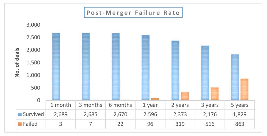
Sustainability 2020, 12, 2999                                                                        2 of 31

attempt to investigate the effect of the time it takes to complete a deal on the post-deal performance
and the likelihood of failure of the acquirer or the newly combined firm.
       Chahine, Hasan and Mazboudi report that according to Mergermarket Group, about 64% of
respondents prefer to complete M&A deals quickly to capture synergies early, and 36% prefer expanding
the due diligence timeline [6]. Thus, we propose and test two complementary hypotheses—the due
diligence hypothesis and the overdue hypothesis—to examine whether the time taken until deal
completion is an indication predicting the performance and survival of a deal post-completion. The due
diligence hypothesis posits that a deal may take a long time to complete after its announcement because
the acquirer has undertaken rigorous due diligence to ensure a proper close. This due diligence process
provides acquiring firms with a more informed assessment of the expected costs, benefits, and risks
of acquisition and grants them the opportunity to renegotiate or terminate bad deals [7]. If the due
diligence hypothesis holds, then the deal should experience higher gains and be associated with a
higher likelihood of survival post-M&A, while deals for which due diligence is not undertaken should
be associated with lower performance outcomes and increased failure likelihood. On the other hand,
the overdue hypothesis posits that a deal may be delayed or abandoned if it faces huge challenges to
successful completion and implementation. In such a situation, the deal is delayed not necessarily
because due diligence is being undertaken, but because of possible challenges to the deal itself; even if
the deal is completed, we expect a higher possibility of poor performance and subsequent deal failure.
Our findings support both of our hypotheses, as we confirm an inverse U-shaped relationship between
time until deal completion and post-M&A performance and a U-shaped relationship between time
until deal completion and post-M&A failure.
       Wangerin shows that less due diligence is associated with lower post-merger profitability and
indicates a monotonic relationship between due diligence and profitability [7]. We show further
in addition to his findings that beyond an optimal deal closing time, the acquirer also suffers low
post-merger profitability indicating the presence of a non-monotonic relationship. Further, our study
takes on the further challenge of using various time intervals from the short term to the long term
(i.e., the immediate one month after the deal close to five years after completion) and in addition uses
additional measures of profitability not limited to Wangerin’s single measure. We also show that there
is a non-monotonic relationship between the time it takes the deal to close, and the likelihood of failure.
       The question of what is the optimum time within which to close a deal is complex, since any
number of deal antecedents and characteristics may affect the time required until a deal closes, such as
the deal’s complexity [8]; whether it is local or cross-border [9]; whether the target has a poor past
performance and has a bankruptcy flag on the deal [10,11]; whether it is a friendly or hostile deal [12];
whether the acquirer’s stocks are overvalued [13]; whether the deal is occurring during a financial
crisis [14]; and what type of deal advisors are involved [15]. To control for the endogeneity of time
until deal completion, we employ an instrumental variable regression to provide further support for
our findings, albeit weakly.
       To the best of our knowledge, this study is the first to test time until deal completion as a
determinant of M&A performance and subsequent survival. We help explain why some M&A fail, in
contrast to the large body of literature suggesting that M&A are a useful way to increase shareholder
value and improve the performance of underperforming targets. We also suggest that time until deal
completion could proxy for a varied array of risk factors influencing survival post-M&A. In a market
where information is typically kept out of the public eye during the negotiation process, the time
taken until deal completion is likely to be a very important source of information for investors, risk
managers, and regulators. Caiazza and Pozzolo indicate that the time elapsed from the moment of the
announcement of a deal and its successful conclusion or its abandonment can provide information on
the ex-ante probability that it will succeed or fail, thus suggesting the need to pay attention to the time
it takes until a deal is completed [16]. Ekelund, Ford and Thornton find that the time difference for
merger completion is estimated to be about 75 days (or 80%) longer in regulated industries and that
both the cost of merger delay and the benefits of careful merger review can be substantial concluding
Sustainability 2020, 12, 2999                                                                          3 of 31

that an interesting extension of their research would be to evaluate why delays exist and their financial
significance [17]. Though our paper does not fully investigate the reasons for delays, our paper is an
attempt to investigate the economic significance of careful merger reviews as against delays which
may provide information on how swift or otherwise dealers need to act to conclude a deal
     The rest of the paper is structured as follows. Section 2 reviews the literature on M&A and
develops the study’s hypotheses. Section 3 describes the data, explains how they were collected, and
introduces the study’s research methodologies. Section 4 presents and describes the results. Finally,
Section 5 concludes the paper.

2. Literature Review and Hypothesis Development
     Rigorous research over the past decade has investigated the determinants of M&A performance
and failure. One of the major purposes of M&A is to take advantage of the synergies created by
joining the two entities, and these synergies are time-bound. Thus, as the literature has stressed, the
deals need to be closed in a timely fashion [6]. In addition, because executives can engage in adverse
behavior while undertaking large acquisitions, many shareholders pressure managers to close their
deals quickly [18]. When deals close too quickly, and without due diligence, they lead to concerns
about their performance and survival. However, due diligence requires time and a large investment of
resources: It is costly. Nevertheless, the research has shown that more due diligence is undertaken by
acquirers when the benefits expected from undertaking such due diligence exceed the expected costs
and when it would lead to a better deal. Furthermore, the M&A market is opaque, and its negotiations
are conducted behind closed doors, so that the public cannot easily ascertain what is happening.
The major events most visible to the market are announcements of deals and of their consummation or
abandonment. Given the information asymmetry between the parties to a deal and the market and the
expectation that a successful deal should close within an optimal period, the time a deal takes to close
could be a valuable source of information and serve as a signal to the market about whether the deal is
potentially value-creating or faces significant challenges, thus, indicating its expected performance and
survival. The focus of our research is on transactional due diligence conducted by the acquirer after
the deal announcement as opposed to preliminary due diligence or due diligence review conducted
before the announcement. To the extent that the acquirer has signed a deal agreement with the target
and announces it to the public, we believe the acquirer would have conducted enough preliminary
due diligence to satisfy itself of the validity of the deal and that further transactional due diligence is
only undertaken by the acquirer for incremental benefits to the deals, ceteris paribus. In this context,
two complementary hypotheses related to the time until completion are proposed below.

2.1. Due Diligence Hypothesis
      Effective due diligence is taken by the acquirer to satisfy itself of the validity of the representation
and warranties made by the target in the deal provisions. Wangerin indicates that due diligence
enables the acquirer to verify that no “material adverse event” has occurred that would be detrimental
to the value of the target firm [7]. He further shows that less due diligence is associated with lower
post-merger profitability. In a rushed deal, detailed provisions critical to its success might be overlooked
or ignored, the targets may conceal earnings management [19], or the acquirers may hide opportunistic
activities, such as inflated earnings [20]. As rushed deals have potentially negative consequences, the
literature has stressed the need for effective due diligence for deal success.
      Therefore, adequate due diligence should ensure increasing returns to the acquirer post-M&A.
We assume in proposing this hypothesis that, in line with prior findings, the acquirer will conduct
due diligence on condition that the expected benefits from the additional effort are greater than the
associated costs, including the direct cost of the due diligence process itself and the indirect cost
of losing timeliness through a delayed close. If these assumptions are correct, a deal’s post-M&A
performance should increase, and its post-M&A likelihood of failure decrease, as the time taken for deal
completion increases, due to the benefits accruing from the additional due diligence efforts. This would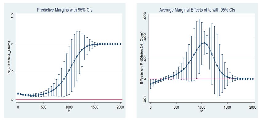
Sustainability 2020, 12, 2999                                                                               4 of 31

indicate an increasing or positive relationship between time until deal completion and subsequent deal
performance and a negative relationship between the former and the likelihood of failure post-M&A.
We, thus, propose the following:

Hypothesis 1: If the due diligence hypothesis holds, there is a positive relationship between time until deal
completion and subsequent deal performance post-M&A up to its optimum closing time, ceteris paribus

Hypothesis 2: If the due diligence hypothesis holds, there is a negative relationship between time until deal
completion and the likelihood of deal failure post-M&A up to its optimum closing time, ceteris paribus.

2.2. Overdue Hypothesis
      As M&A are complex, sufficient time and resources must be committed to ensure the expected
outcome. Differing from deal to deal, this sufficiency is defined as the optimal time required for the deal
to close and for optimal due diligence by the acquirer. However, if a deal takes a longer-than-optimum
time to implement, the loss of timeliness and expected deal synergies would reduce performance and
increase the risk of failure. The literature lists a number of reasons why a deal may be delayed, including
conflicting interests among the parties during negotiations; government influence via antitrust laws;
and the opposition of stakeholders, such as shareholders, employees, and interested social groups.
Thus, when a deal takes longer than its optimum interval to close, even if the delaying factors are
not revealed to the market, the delay may indicate challenges, problems, or opposition to the deal.
The rising and prohibitive termination fees associated with the inability to close a deal may be an
important reason why parties to a deal, especially the acquirer, may want to see a deal to the end
even if it encountered problems during the negotiation process [21]. We hypothesize that this delay
will reduce subsequent performance after the deal closes because of the risk that the fundamentals
of the target may change substantially from what was envisaged [1], and the risk that an untimely
implementation will subtract from the deal the beneficial synergies of integration, such as technological
advancements and tax credit consolidation. This suggests a negatively sloped relationship between
time until deal completion and subsequent performance if a deal is delayed beyond the optimal closing
time and a positively sloped relationship with the subsequent likelihood of failure: As time until deal
completion approaches its optimum, subsequent performance increases until it reaches a maximum
at the optimum and decreases as the deal is delayed further beyond the optimum time; the opposite
dynamic obtains concerning the likelihood of failure. We, thus, propose the following:

Hypothesis 3: If the overdue hypothesis holds, there is a negative relationship between time until deal completion
and subsequent deal performance post-M&A beyond its optimum closing time, ceteris paribus.

Hypothesis 4: If the overdue hypothesis holds, there is a positive relationship between time until deal completion
and the likelihood of deal failure post-M&A beyond its optimum closing time, ceteris paribus.

      The due diligence and overdue hypotheses are complementary, rather than competing. Rather
than the relationship between time until deal completion and subsequent performance continuously
being positive or negative, we argue that it is positive only up to an optimum point and then negative
thereafter. The opposite effect holds for the relationship between time until deal completion and the
likelihood of failure. Specifically, we propose, there is an inverse U-shaped relationship between time
until deal completion and post-M&A performance and a U-shaped relationship between time until
deal completion and the post-M&A likelihood of failure. We, therefore, test hypotheses 1 and 3 and
hypotheses 2 and 4 together with a quadratic term in our regressions.
      There is few research that discusses the time until deal completion and its effect on post M&A
performance or failure. Most of the literature does not explicitly test for this, albeit we find discussions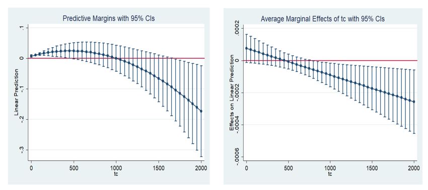
Sustainability 2020, 12, 2999                                                                                                    5 of 31

or indication in them that help buttress our hypothesis. We have attempted to summarize some of
them in Table 1 below.

                                       Table 1. List of articles related to hypotheses.

          Author (Year)                                                  Relation to Hypothesis
                                           Hypothesis 1 and 2: Due Diligence Hypothesis
                                       Based on an analysis of the time to negotiate an acquisition agreement and complete the
                                      transaction, the author predicts, and finds, that competitive pressures, short-term financial
                                    reporting incentives, and agency problems are associated with less due diligence and that less
      1. Wangerin (2017) [7]
                                      due diligence is associated with lower post-acquisition profitability, a higher probability of
                                    acquisition-related goodwill impairments, and lower quality fair value estimates for the acquired
                                      assets and liabilities. This suggests the need for acquirers to conduct enough due diligence.
                                    In this paper, the author indicates that the extended time from announcement to completion will
       2. Fuller (2003) [22]        allow for target and bidder uncertainty to be resolved prior to the closing. This also suggests the
                                                                 need for due diligence to be conducted.
  3. Caiazza and Pozzolo (2016)     Authors indicate that deals which are profitable for both parties involved are likely to be closed
               [16]                 quickly. This suggests that if deals are, indeed, of good quality, they will not be unduly delayed.
                                         Authors argue that since there is generally a delay between the announcement and the
                                    completion of a merger, subsequent news, disclosures, and earnings announcements can bring
                                    renewed attention to the acquirer and dilute the potential benefit associated with the timing of
                                    the merger announcement if the deal is overvalued. Therefore, managers are more likely to act
   4. Louis and Sun (2016) [20]     opportunistically when they anticipate the mergers to be completed relatively fast, and in some
                                     instances, speed up the approval process to minimize the lag between the announcement and
                                    the completion dates, since protracted negotiations, and public attention increase the odds that
                                    the overvaluation would be exposed. The foregoing strongly suggests the need for due diligence
                                      to avoid the acquirer overpaying for the deal and to unearth opportunistic acts of managers.
                                              Hypothesis 3 and 4: Overdue Hypothesis
                                    Firm value can change substantially between the time deal terms for a public target are set and
                                        closing, risking renegotiation or termination. Authors find increases in market volatility
                                     decrease subsequent deal activity, and the effect is strongest when volatility is highest and for
 1. Bhagwat, Dam and Harford
                                    deals taking longer to close, making merging parties attempt to shorten the interim window as
          (2016) [1]
                                      risk increases. Thus, they demonstrate that longer time to completion is responsible for an
                                    increase in merger uncertainty. From the foregoing, it can be projected that delaying the closure
                                                                       of the deal is not beneficial.
                                    The authors stated that the basic economic justification for a transaction is not likely to change
    2. Muehlfeld, Sahib and            fundamentally between its initiation and completion unless very long time intervals are
    Witteloostuijn (2007) [23]      involved. This suggests that if very long intervals are involved, the economic justification may
                                                   be eroded, and deals may no more be beneficial to the acquirer.
                                    According to authors, delays in M&A completion can result in rising expenditures, and merger
 3. Luypaert and De Maeseneire
                                       delays implicate a loss of focus. This could cause the company to miss out on business
           (2015) [8]
                                             opportunities suggesting the need to avoid delays in completing the deal.
                                     Authors indicate that the time duration of the evaluation and negotiation of the target firm is
 4. Ferreira, Borini, Vicente and
                                    relevant, due to the costs incurred and the opportunity costs of not pursuing other alternatives
       Almeida (2017) [24]
                                                                suggesting the need to close deals quickly.
                                     According to authors, direct costs like negotiation or advising will keep increasing, due to the
  5. Hwang and Roh (2014) [25]      longer time to completion. They can even increase to a point where they could not be offset by
                                                                      the post-M&A performance.
                                      Author discusses that limiting deal duration can help the acquirer focus faster on its daily
                                      operations preventing the company from missing out on future business opportunities. In
      6. Picquet (2017) [26]            addition, competitors are kept out of the game, due to the short time allowed to react.
                                    Shareholders can enjoy from faster completion by having the benefits (synergies, market power,
                                                          etc.) flowing out of the M&A transaction quicker.
                                            Source: Authors’ literature survey (2020).

3. Data

3.1. Sample Selection
    Data for this study are obtained from a wide variety of sources. We collect data on both local
US M&A and cross-border M&A from 2000 to 2010 between US firms as acquirers and firms in other
countries as targets from the Thomson Reuters Securities Data Company (SDC) Platinum Mergers and
Acquisitions database. Since we use data from the anti-director index developed by Djankov et al. [27],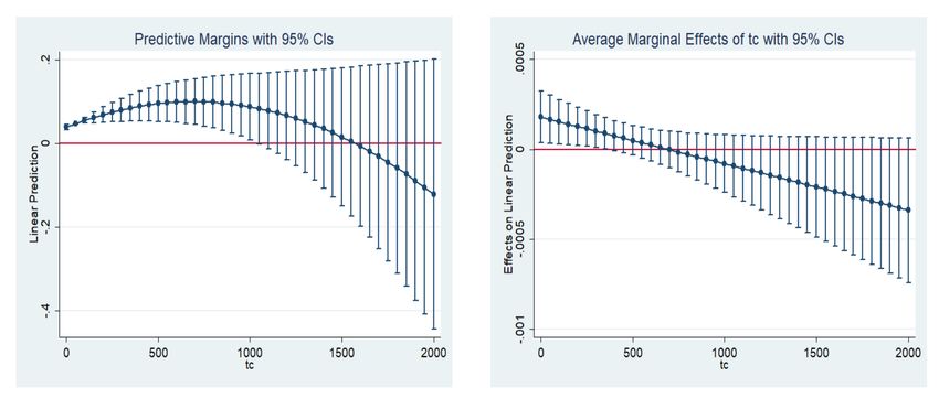
Sustainability 2020, 12, 2999                                                                      6 of 31

the target countries comprise the 73 countries examined in their study. We include only completed deals
and exclude deals involving governments or their agencies, as well as unknown deals. The sample
includes both public and private targets. Data on the following deal characteristics were obtained:
Date announced, date effective, post-acquisition ownership percentage, value of transaction, target and
acquirer SIC codes, form of deal compensation (percentage of stock or percentage of cash), the attitude
of the deal (whether friendly or hostile), and the number of target and acquirer advisors. We collect
data on stock returns and information on delisting from the Center for Research in Security Prices
(CRSP) and data on firm fundamentals from COMPUSTAT.
      The following control variables are used. At the deal level, we control for performance and
survival effects related to payment method using a dummy variable that equals one if the deal is
majority financed by cash, and zero otherwise. Berkovitch and Narayanan [28] have shown that
cash-financed deals can be accomplished quickly without delays, thus, posing less risk to the deal;
the opposite is true when the deal is financed with stock or a mixture of securities. The ownership
percentage determines whether the acquirer can control the target. If the acquirer does not have
majority control, the inefficiencies currently causing poor target performance are highly likely to
continue, as there is no definite change in ownership to affect performance or survival probability [29].
Research has shown that M&A between firms in unrelated industries are usually associated with poor
performance because such mergers rarely benefit from the advantages generated by sharing resources,
having experience in the same industry, and enjoying an easy availability of human resources, among
others [30].
      With respect to country-level controls, weaker shareholder protection poses a risk to the
performance and survival of an M&A deal because of the high costs of expropriation and lower
stock development, creating friction in the raising of external equity [31]. Bebchuk [32] shows how low
shareholder protection negatively affects corporations and shareholders. We control for shareholder
protection using the anti-director rights index of Djankov et al. [27]. The finance literature has shown
that cultural differences between countries can affect business dealings between them [33,34]. We, thus,
control for how differences between the advisor and target countries’ cultures in terms of language and
religion can affect the M&A deal. Countries’ locations and the distance between them influence their
culture, weather conditions, and the ease with which business can be conducted between them. There
are benefits to geographical diversification in the form of increased markets, exposure to different
economic conditions, and the opportunity to learn new skills and obtain new resources and technology.
However, it has been empirically shown that differences in geographical location between the acquirer
and target can affect M&A deals [35]. We control for these differences using a geographical dummy.
We, thus, use GDP growth and total stock market development growth to control for other possible
country and capital market effects.

3.2. Testing for U-shaped and Inverted U-shaped Relationship and Optimal Turning Point
      In recent years, much attention has been paid to the consequences of spurious quadratic
relationships concluded merely based on the significance and magnitude of the unsquared and
squared terms in a model. Consequently, more stringent tests for verifying the robustness of findings
of quadratic relations have been developed and applied in the literature. We use the rigorous test of
Lind and Mehlum [36] to test the U-shaped and inverse U-shaped relationships we have hypothesized
(The tests are referred to as U-test in the reported tables). An inverse U-shaped quadratic relationship
requires a positive slope at the start and a negative slope at the end of the interval and vice versa.
We set the minimum and maximum values to the observed values in our sample. We set a quadratic
relation of the form:
                                       y = α + β1 tc + β2 tc2 + γ0 z + ε                             (1)

where tc is the explanatory variable time until deal completion, y is the variable to be explained
(i.e., CAR, BHAR, ∆TURNOVER, and ∆ROA as defined in Appendix A), ε is the error term, and z is
the set of control variables (also defined in Appendix A).
Sustainability 2020, 12, 2999 7 of 31
Suppose σ11 is the estimated variance of β̂1 , σ22 is the estimated variance of 2β̂2 , and σ12 is the
estimated covariance of β̂1 and 2β̂2 , where β̂1 and β̂2 are the estimators of β1 and β2 , respectively.
The null and alternative hypotheses for testing an inverse U-relationship are
H0 : β1 + 2β2 tcmin ≤ 0, H0 : β1 + 2β2 tcmax ≥ 0 (2)
Ha : β1 + 2β2 tcmin > 0 > β1 + 2β2 tcmax (3)
where tcmin is the minimum time to close the deal and tcmax is the maximum time to close the deal in
our sample. The corresponding t-statistic is
β̂1 + 2β̂2 tc j
tj = q 2 , j = min or max. , (4)
σ11 + 2σ12 + σ22 tc j
In addition, from the quadratic relation defined above, it follows with a simple differentiation that
the optimal time for closing the deal should occur at the time where
β1 + 2β2 tc = 0 (5)
Put differently, this occurs at the turning point; the point where the average marginal effect
equals zero.
In addition, we make use of a Wald test to investigate the significance of including the squared
term of time until deal completion in our regressions. The null of the Wald test is that the squared term
is zero. If it is rejected, then it indicates that placing a squared term in the regressions is justifiable and
relevant as we do. Otherwise, it means the squared term of time until deal completion can be deleted
without affecting our model in any meaningful way.
3.3. Measuring Stock Performance
We use the standard event study measure to evaluate the firm’s stock performance after the close
of the deal. We use the cumulative abnormal return (CAR) as the measure during the short-horizon
study and the buy-and-hold abnormal return during the long-horizon study. The cumulative abnormal
return of the acquirer is computed as
T
X
CARi = (Rit − E(R it )) (6)
t=1
where R it is the return of the acquirer, and E(R it ) is the expected return of the acquirer computed
based on the mean-adjusted model, market model, three-factor model of Fama and French [37], and
four-factor model of Carhart [38]. The buy-and-hold abnormal returns (BHAR) of the acquirer are
computed as
YT YT
BHARi = (1 + Rit ) − (1 + E(Rmt )) (7)
t=1 t=1
where R it is the return of the acquirer and E(R mt ) is the expected return of the market portfolio.
The value-weighted return of all CRSP firms incorporated in the US and listed on the NYSE,
AMEX, or NASDAQ is used as a proxy for the market return.
The market model is estimated as Rit = αi + βi Rmt + Eit , with Rit being the return of the acquirer
in the estimation window and Rmt the corresponding value-weighted return of all CRSP firms and
E[Eit ]= 0.
The three-factor model is estimated as (Rit − r f t ) = αi + βi,m Rmt − r f t + βi,smb SMBt +
βi,hml HMLt ) + Eit ., with E[Eit ]= 0, where Rit is the return of the acquirer in the estimation window,Sustainability 2020, 12, 2999 8 of 31
r f t is the risk-free rate, Rmt is the corresponding value-weighted return of all CRSP firms, SMBt is the
excess return of small over big stocks measured by market capitalization, HMLt is the excess return of
high market-to-book ratio stocks over low market-to-book ratio stocks.
The four-factor model is estimated as (Rit − r f t ) = αi + βi,m Rmt − r f t + βi,smb SMBt + βi,hml HMLt ) +
βi,mom MOMt ) + Eit , with E[Eit ]= 0, where Rit is the return of the acquirer in the estimation window,
r f t is the risk-free rate, Rmt is the corresponding value-weighted return of all CRSP firms, SMBt is the
excess return of small over big stocks measured by market capitalization, HMLt is the excess return of
high market-to-book ratio stocks over low market-to-book ratio stocks, MOMt is the excess of past
winning stocks over past losing stock (also referred to as the “momentum factor”).
3.4. Sample Summary and Description
We summarize and describe the sample in Table 2. The summary of deals by target nation and the
correlation table of the variables used in the study are reported additionally in Appendix B. Our sample
consists of 5925 firm-year observations and 2689 firms. The highest number of observations occur in
2000, and the next highest number occurred in 2006. This is consistent with the observation in the
literature that M&A activity rose through the early 2000s until the onset of the financial crisis in 2007.
In terms of continental classification, most of the deals occur in the Americas (probably influenced by
the large number of observations of local US M&A in our sample), and the next highest number occur
in Europe. As reported in Appendix B under deal summary by target nation based on effective year,
the highest number of international deals occur between the US and Canada and between the US and
the United Kingdom, reinforcing the finding of other studies that more M&A occur between countries
that are geographically close or that have a large volume of bilateral trade.
Panel B of Table 2 shows that the mean time it takes to complete a deal is about two months,
and the longest duration in our sample is sixty-six months (corresponding to about five years and six
months). The shortest time is zero, which represent deals that are completed on the same day they are
announced. Note that this does not imply that the acquirer did not undertake any due diligence at
all as the acquirer could have already undertaken some preliminary due diligence or due diligence
review before the deal announcement, albeit our focus is on transactional due diligence conducted
after the deal announcement. Another variable of interest is the ownership percentage; the mean is
about 98.53%.
This ownership level indicates that the acquirer has obtained enough ownership in the target to
control it completely and that the performance of the target can have a material effect on the acquirer
post-M&A.
The correlation table reported in Appendix B indicates that the pairwise correlation between the
variables in our sample is substantially low. The highest correlation is between the language dummy
and the geographical dummy. This is not a cause for concern. The mean variance inflation function of
our variables is 2.09, far below the rule-of-thumb of 10 used in many studies. Therefore, our study has
no multicollinearity issues. In addition, the Breusch–Pagan/Cook–Weisberg test and the White test for
heteroscedasticity with a null of constant variance are rejected, indicating possible heteroscedasticity
in our models. We, thus, use heteroscedasticity-robust standard errors. We also correct for possible
clustering at the firm and year levels. The mean level of Tobin’s Q is 1.95, indicating that the acquiring
firms in the sample are overvalued on average. The acquirers’ mean debt-to-asset ratio is also 0.48;
it can, thus, be inferred that most of the acquirers are not saddled by significant debt; their assets can
cover twice their level of debt in their portfolios on average.Sustainability 2020, 12, 2999 9 of 31
Table 2. Summary and descriptive statistics.
Panel A. Deal Summary by year, Continent, and Type
Year of Completion Frequency Percent Continent Frequency Percent
2000 630 10.63 Africa 9 0.15
2001 572 9.65 America 5,103 86.13
2002 577 9.74 Asia 157 2.65
2003 530 8.95 Europe 594 10.03
2004 577 9.74 Oceania 62 1.05
2005 574 9.69 Total 5925 100
2006 596 10.06
2007 581 9.81
2008 481 8.12
2009 348 5.87
2010 403 6.8
2011 51 0.86
2012 2 0.03 Type Frequency Percent
2013 2 0.03 US local 4827 81.47
2014 1 0.02 International 1098 18.53
Total 5925 100 Total 5925 100
Panel B. Descriptive Statistics
Variable N Mean Standard Deviation Minimum Maximum
Time until completion (months) 5925 1.77 3.035 0 66.267
GDP growth 5925 2.23 1.997 −10.894 15.24
Total stock growth 5925 0.134 0.465 −1 14.495
Value of transaction 5925 3.669 1.932 −5.116 11.194
Ownership percentage 5925 98.527 7.83 11 100
Size 5925 6.563 1.917 0.474 13.59
Cash 5925 0.117 0.129 0 0.949
Debt 5925 0.478 0.238 0.005 2.775
Tobin’s Q 5925 1.949 1.444 0.22 35.099
Shareholder protection 5925 0.642 0.112 0.092 1
Number of acquirer advisors 1835 1.189 0.542 1 9
Number of target advisors 2425 1.16 0.451 1 5
Figure 1 reports the cumulative abnormal returns of the acquirer after the deal closes and becomes
effective. Specifically, we report the CAR for two days before and two days after the effective date,
as well as for 10 days before and 10 days after it. We employ various approaches to measure the
expected returns, such as using the mean-adjusted return, market-model, Fama–French three-factor
model, and Carhart four-factor model. Aside from the mean-adjusted model, which shows higher
levels of cumulative abnormal returns of about 0.92% for the (−2,2) day interval, very little difference
is seen when using the other three approaches; they show about 0.45% cumulative abnormal returns
for the same interval. The models all show similar abnormal return trends. The acquirer experiences
increasing returns around the day the deal closes, and then they begin to decrease. The increase in
returns beyond what is expected for the acquirer when the deal closes indicates a positive reaction
from the market that the deal has closed successfully, allaying uncertainties regarding whether the
deal would be abandoned. This result is a confirmation of prior findings in the literature of a positive
reaction associated with a successful close [39].Sustainability 2020, 12, 2999 10 of 31
Figure 1. Cumulative abnormal returns of the acquirer (−2,2) and (−10,10) using the mean-adjusted
model, market-model, Fama–French three-factor model and Carhart four-factor model. Source:
Thomson Reuters Securities Data Company (SDC) Platinum Mergers and Acquisitions database, Center
for Research in Security Prices (CRSP) database.
4. Results and Discussion
To investigate how the time until completion affects the acquirer post-M&A, we study
several quantitative indicators, including stock performance, financial performance, and operational
performance. We also investigate how time until deal completion affects the likelihood of failure, and
then conduct a survival analysis.
4.1. Stock Performance
Table 3 presents the results of our tests for the due diligence and overdue hypotheses using stock
performance. For the short-term analysis, we use cumulative abnormal return (CAR) to measure
the stock performance of the acquirer one month and three months after the deal, as in Equation (8).
Due to the misspecification bias related to using CAR to measure long-horizon returns, we adopt the
buy-and-hold abnormal returns (BHAR) to measure stock performance six months, one year, two
years, and three years after the deal following Kothari and Warner [40], as in Equation (9). In this study,
we focus on the post-merger CAR and BHAR because the acquirer was independent of the target at the
announcement date. The deal is effective only after the deal closes or is consummated. To estimate
the expected returns, we use the constant mean-adjusted model for all subsequent regressions after
confirming that our results do not substantially differ across the different measurement approaches
outlined above. We run a panel regression using a squared term of time until completion to test the
inverse U-shaped relationship between stock performance and time until deal completion:
CARit = α + β1 ∗ tcit + β2 ∗ tcit 2 + γ0 Control variablesit + µi + εit (8)
BHARit = α + β1 ∗ tcit + β2 ∗ tcit 2 + γ0 Control variablesit + µi + εit (9)
where CAR is the cumulative abnormal returns of the acquirer or newly merged firm, tc is the time
until deal completion, tc2 is the squared term of time until deal completion, µi are firm fixed effects
used to control for time-invariant heterogeneity among firms, and ε is the error term. The control
variables are the national- and firm-level and deal-specific variables, as explained above. All variables
are defined in Appendix A. The Wald tests to verify that the quadratic terms in the models are equal
to zero are reported. In addition, the turning point of the quadratic relationship between time until
deal completion and the dependent variable is reported, as well as the result and implication of theSustainability 2020, 12, 2999 11 of 31
stringent test of quadratic relation, following Lind and Mehlum [36]. Standard errors are corrected for
heteroscedasticity and clustered by firm and year.
Table 3. Effect of Time until Completion on Stock Performance.
Dependent Variable: (1) (2) (3) (4) (5) (6)
CAR/BHAR 1 MONTH 3 MONTHS 6 MONTHS 1 YEAR 2 YEARS 3 YEARS
Time 0.0023* 0.0071** 0.0077** 0.0131* 0.0217** 0.0308**
(0.082) (0.012) (0.034) (0.087) (0.034) (0.019)
Time squared −0.0001*** −0.0002*** −0.0002** −0.0002* −0.0006** −0.0006***
(0.008) (0.001) (0.011) (0.078) (0.029) (0.003)
Cash payment 0.0070* 0.0080 0.0242* 0.0304 0.0241 0.0227
(0.059) (0.290) (0.098) (0.110) (0.439) (0.567)
Industry difference −0.0067 −0.0113 −0.0327*** −0.0440* −0.0430* −0.0413
(0.336) (0.181) (0.005) (0.067) (0.076) (0.120)
Shareholder protection 0.0921*** 0.0731 0.2083* 0.5465* 0.3725* 0.4425
(0.001) (0.235) (0.050) (0.094) (0.060) (0.126)
Language difference 0.0344** 0.0309 0.1165* 0.2824 0.1211 0.1899
(0.032) (0.350) (0.063) (0.101) (0.299) (0.334)
Geographical difference −0.0066 0.0009 −0.0415 −0.1181* −0.0274 −0.0428
(0.521) (0.962) (0.182) (0.083) (0.601) (0.622)
GDP growth −0.0026 −0.0056* −0.0096** −0.0071 −0.0118 −0.0063
(0.105) (0.071) (0.037) (0.505) (0.189) (0.575)
Total stock growth −0.0070 −0.0013 −0.0039 −0.0151 −0.0108 −0.0280
(0.307) (0.853) (0.746) (0.378) (0.622) (0.390)
Ownership percentage 0.0003 0.0001 −0.0003 −0.0046 0.0008 0.0033***
(0.394) (0.824) (0.644) (0.122) (0.459) (0.003)
Value of transaction −0.0015 −0.0079** −0.0133*** −0.0210** −0.0271** −0.0447***
(0.374) (0.023) (0.009) (0.027) (0.022) (0.008)
Size −0.0146* −0.0321** −0.0913*** −0.2456*** −0.5374*** −0.7691***
(0.056) (0.018) (0.000) (0.000) (0.000) (0.000)
Cash flow 0.0863*** 0.1653*** 0.2316** 0.2939* 0.0693 0.1322
(0.001) (0.004) (0.027) (0.068) (0.785) (0.751)
Debt 0.0159 0.0300 0.2137*** 0.3708*** 0.8064*** 1.3637***
(0.582) (0.515) (0.002) (0.004) (0.000) (0.000)
Tobin’s Q 0.0166*** 0.0316*** 0.0429*** 0.0032 −0.0916*** −0.1487***
(0.000) (0.000) (0.000) (0.842) (0.000) (0.000)
Constant −0.0251 0.1010 0.3456** 1.5970*** 3.2025*** 4.4515***
(0.686) (0.357) (0.032) (0.000) (0.000) (0.000)
Firm fixed effect Y Y Y Y Y Y
Observations 5,921 5,914 5,888 5,747 5,322 4,928
R-squared 0.030 0.042 0.064 0.083 0.143 0.145
Number of firms 2,689 2,686 2,671 2,598 2,376 2,180
Extremum of time
455 477 664 801 543 816
until completion(days)
Wald test:
Rejected Rejected Rejected Marginal Rejected Rejected
Time squared = 0
U-test Null Monotone/U Monotone/U Monotone/U Monotone/U Monotone/U Monotone/U
U-test (P-value) 0.046 0.0006 0.0166 0.0819 0.00661 0.00588
Strong Strong Strong Weak Strong Strong
U-test-implication
Inverse-U Inverse-U Inverse-U Inverse-U Inverse-U Inverse-U
P-value is in parentheses. *** p < 0.01, ** p < 0.05, * p < 0.1. Rejection of the Wald test at p < 0.05, while its marginal
rejection is at p < 0.1.
The results are shown in Table 3 indicate a negative sign on the squared term of time until deal
completion, confirming an inverse U-shaped relationship. We subject the model to the stringent test of
Lind and Mehlum [36]. The null hypothesis of monotone or U-shaped relationship is strongly rejected,
indicating an inverse U-shaped relationship between time until deal completion and stock performance,
and thus, confirming hypotheses 1 and 3. In other words, the results are shown in Table 3 support
both the due diligence hypothesis and the overdue hypothesis. This result implies that, up until a
certain optimal period of deal completion, post-M&A stock performance measured by cumulative
abnormal returns or buy-and-hold abnormal returns increases until it reaches a maximum; when timeSustainability 2020, 12, 2999 12 of 31
until deal completion extends beyond this optimal time, however, stock performance declines, as the
possible existence of challenges to the deal is being signaled. The results for various time intervals
show that our findings are robust to various time specifications. The Wald test that the quadratic term
in the model is zero is strongly rejected in all time intervals except for one year after deal completion,
where it is marginally rejected at the 10% level. Interestingly, the extremum revealed empirically in our
sample for the one-month interval is 455 days (one year and three months), which is far beyond the
mean period of about two months for deal completion in our sample. This indicates that deals that
should take an average of about two months, but that extend beyond one year arouse concern in the
market given the opaque nature of information provision during the negotiation process, coupled with
the desire to close deals quickly to benefit from timely synergies.
When seeking to determine the economic impact of time until deal completion on stock
performance, we cannot directly employ the magnitude of the coefficients of time and time-squared in
the models. The literature agrees that the co-efficient of a quadratic term in a model is not equal to the
marginal effect, in contrast to the case of a normal linear regression without any polynomial terms or
interaction terms. This applies not only to squared terms, but also to other polynomial terms, as well
as interaction terms in any empirical model. This issue is further complicated if the regression is a
non-linear one, such as the probit or logit regression [41]. We, therefore, present a graphical illustration
of how time until deal completion affects the acquirer’s stock performance at various durations until
deal close in Figure 2 for the one-month interval. As presented in the predictive margins graph
of Figure 2, there is a clear inverse U-shaped relationship between time until deal completion and
stock performance. As time until deal completion increases toward the turning point, the acquirer’s
abnormal stock returns increase, but they begin to decrease beyond the extremum. Regarding marginal
effects, for deals that close up until the turning point of about 455 days, every additional day adds a
positive abnormal return to the firm’s overall stock performance until an extremum, thus, lending
support to the due diligence hypothesis. However, beyond the extremum, every additional day adds a
negative abnormal return to the stock performance, resulting in a decreasing slope and a decline in
performance, supporting the overdue hypothesis.
Figure 2. Predictive margins and average marginal effects of time until completion (in days) on
acquirer’s cumulative abnormal returns one month after the close of the deal with 95% confidence
intervals. Source: Table 3.
Concerning the other control variables, our results confirm the literature in many ways. Deals
paid for in cash are positively related to subsequent acquirer performance, though not significantly, in
our sample. The literature generally finds that deals that are expected to result in large gains for the
acquirer and in which the acquirer is confident are paid for in cash to prevent the target’s shareholders
from benefitting from the increases in share prices that would result if they were paid for in stock.Sustainability 2020, 12, 2999 13 of 31
Differences across industries and geographical locations are associated with negative coefficients, as
expected. The coefficient on shareholder protection in the target country is positive, indicating that
M&A involving target countries with strong shareholder protection are associated with increases in
overall share performance and less risk of expropriation from acquirers’ gains, which strongly aligns
with both our intuition and the literature. Given the widespread criticism in the literature of using
stock performance alone to measure performance, we present further evidence using the acquirer’s
post-deal operational and financial performance.
4.2. Operational Performance
We measure operational performance using the change in turnover as a proxy. Thanos and
Papadakis [42] show that this proxy is used in the accounting literature as an alternative approach
to measuring operational performance or efficiency. We expect an increase in turnover for deals that
improve the acquirer’s operational performance post-M&A. We run a panel regression controlling for
firm fixed effects, as in the model in Equation (10), below:
∆TURNOVERit = α + β1 ∗ tcit + β2 ∗ tcit 2 + γ0 Control variablesit + µi + εit (10)
where TURNOVER is the sales scaled by total assets of the acquirer or newly merged firm t-years
after, tc is the time until deal completion, tc2 is the squared term of time until deal completion, µi
are firm fixed effects used to control for time-invariant heterogeneity among firms, and ε is the error
term. The control variables are the national- and firm-level and deal-specific variables, as explained
above. All variables are defined in Appendix A. The Wald tests verifying that the quadratic terms in
the models are equal to zero are reported. In addition, the turning point of the quadratic relationship
between time until deal completion and the dependent variable is reported, as well as the result and
implication of the stringent test of quadratic relation, following Lind and Mehlum [36]. Standard errors
are corrected for heteroscedasticity and clustered by firm and year.
The results of this regression are presented in Table 4 below. The results for one year and three years
after deal completion indicate an inverse U-shaped relationship between time until deal completion
and operational performance, reinforcing our previous results. The results for two and five years after
the deal reject the inverse U-shaped relationship in the stringent test. The corresponding predictive
margins and marginal effect graphs for one year after the deal are shown in Figure 3. The summary
(albeit weak) evidence is that the due diligence and overdue hypotheses are complementary and are
supported with respect to operational performance.
Figure 3. Predictive margins and average marginal effects of time until completion (in days) on acquirer
turnover one year after the close of the deal with 95% confidence intervals. Source: Table 4.Sustainability 2020, 12, 2999 14 of 31
Table 4. Effect of time until completion on operational performance.
Dependent Variable: (1) (2) (3) (4)
∆TURNOVER 1 YEAR 2 YEARS 3 YEARS 5 YEARS
Time 0.0054** 0.0052* 0.0090** 0.0022
(0.022) (0.089) (0.044) (0.401)
Time squared −0.0001* −0.0001 −0.0002 −0.0001
(0.071) (0.275) (0.137) (0.305)
Cash payment 0.0013 −0.0056 0.0074 −0.0100
(0.899) (0.638) (0.620) (0.353)
Industry difference 0.0063 0.0032 0.0161 0.0184
(0.713) (0.848) (0.315) (0.412)
Shareholder protection −0.1629*** −0.1248 −0.1465* −0.0714
(0.010) (0.146) (0.088) (0.475)
Language difference −0.0673** −0.0625 −0.0551 −0.0134
(0.034) (0.199) (0.232) (0.825)
Geographical difference 0.0119 0.0405 0.0332 −0.0141
(0.356) (0.124) (0.109) (0.590)
GDP growth 0.0084* 0.0081 0.0085** 0.0115*
(0.056) (0.173) (0.026) (0.055)
Total stock growth 0.0039 −0.0311*** −0.0279** −0.0207
(0.670) (0.000) (0.021) (0.243)
Ownership percentage 0.0014** 0.0004 −0.0005 −0.0002
(0.018) (0.789) (0.764) (0.938)
Value of transaction 0.0082** 0.0051 0.0049 0.0110***
(0.021) (0.252) (0.308) (0.001)
Size 0.0711*** 0.0762*** 0.0696*** 0.1070***
(0.000) (0.000) (0.004) (0.000)
Cash flow −0.0856 −0.1025 −0.1880* −0.1603
(0.208) (0.203) (0.080) (0.124)
Debt 0.0976** −0.0087 −0.0267 −0.0926
(0.010) (0.879) (0.682) (0.225)
Tobin’s Q −0.0115** −0.0243*** −0.0295*** −0.0119
(0.025) (0.000) (0.000) (0.184)
Constant −0.5257*** −0.3943* −0.2408 −0.6065*
(0.000) (0.098) (0.323) (0.068)
Firm fixed effect Y Y Y Y
Observations 5538 5152 4794 4193
R-squared 0.051 0.041 0.043 0.046
Number of firms 2491 2293 2109 1801
Extremum of time until
691 842 646 342
completion(days)
Wald test:
Rejected Not rejected Not rejected Not rejected
Time squared=0
U-test null Monotone/U Monotone/U Monotone/U Monotone/U
U-test (P-value) 0.0497 0.195 0.10 0.252
Strong Weak
U-test-implication Monotone/U Monotone/U
Inverse-U Inverse-U
P-values are in parentheses. *** p < 0.01, ** p < 0.05, * p < 0.1. Rejection of the Wald test at p < 0.05, while its
marginal rejection is at p < 0.1.Sustainability 2020, 12, 2999 15 of 31
4.3. Financial Performance
We deepen our analysis of post-M&A performance by employing a measure of financial
performance proxied by the change in return on assets (ROA) as measured by the change in earnings
before interest, taxes, depreciation and amortization (EBITDA) scaled by total assets [42]. We employ a
panel regression, as in Equation (11), and control for firm fixed effects and correct standard errors for
heteroscedasticity and serial correlation, as above.
∆ROAit = α + β1 ∗ tcit + β2 ∗ tcit 2 + γ0 Control variablesit + µi + εit . (11)
where ROA is the earnings before interest, taxes, depreciation and amortization (EBITDA) scaled by
total assets of the acquirer or newly merged firm t-years after, tc is the time until deal completion,
tc2 is the squared term of time until deal completion, µi are firm fixed effects used to control for
time-invariant heterogeneity among firms, and ε is the error term. The control variables are the
national- and firm-level and deal-specific variables, as explained above. All variables are defined
in Appendix A. The Wald tests verifying that the quadratic terms in the models are equal to zero
are reported. In addition, the turning point of the quadratic relationship between time until deal
completion and the dependent variable is reported, as well as the result and implication of the stringent
test of quadratic relation, following Lind and Mehlum [36]. The results are presented in Table 5 and
graphically in Figure 4, below.
Figure 4. Predictive margins and average marginal effects of time until completion (in days) on
acquirer’s return on assets one year after the close of the deal with a 95% confidence interval. Source:
Table 5.
The results are shown in Table 5 support hypotheses 1 and 3 for the time intervals of one, two,
and three years post-deal. However, the null of monotone or U-shaped relationship between time and
financial performance cannot be rejected for the interval of five years after deal completion. All the
foregoing results confirm that the due diligence hypothesis (hypothesis 1) and the overdue hypothesis
(hypothesis 3) are complementary given the presence of an inverse U-shaped relationship between
time until deal completion and post-M&A performance.Sustainability 2020, 12, 2999 16 of 31
Table 5. Effect of time until completion on financial performance.
Dependent Variable: (1) (2) (3) (4)
∆ROA 1 YEAR 2 YEARS 3 YEARS 5 YEARS
Time 0.0025*** 0.0032* 0.0018 0.0013
(0.003) (0.069) (0.189) (0.276)
Time squared −0.0001*** −0.0002*** −0.0001* −0.000016
(0.001) (0.001) (0.058) (0.676)
Cash payment −0.0005 −0.0004 −0.0015 0.0006
(0.879) (0.953) (0.804) (0.919)
Industry difference −0.0044 −0.0043 −0.0022 0.0048
(0.175) (0.436) (0.627) (0.161)
Shareholder protection −0.0084 −0.0931 −0.0223 −0.0363
(0.741) (0.273) (0.689) (0.485)
Language difference 0.0001 −0.0359 0.0019 −0.0090
(0.992) (0.332) (0.930) (0.663)
Geographical difference 0.0036 0.0185 0.0002 0.0035
(0.574) (0.342) (0.990) (0.791)
GDP growth −0.0017 −0.0015 −0.0013 −0.0008
(0.294) (0.328) (0.355) (0.508)
Total stock growth −0.0022 −0.0072 −0.0062 −0.0011
(0.614) (0.145) (0.242) (0.696)
Ownership percentage 0.0003** 0.0004** 0.0003 0.0003
(0.018) (0.028) (0.207) (0.208)
Value of transaction 0.0001 0.0005 0.0021 0.0017
(0.955) (0.793) (0.245) (0.345)
Size −0.0228*** −0.0262*** −0.0255*** −0.0291***
(0.000) (0.000) (0.000) (0.002)
Cash flow 0.0134 −0.0111 0.0141 −0.0347
(0.733) (0.844) (0.718) (0.309)
Debt 0.1401*** 0.1435*** 0.1292*** 0.0892**
(0.000) (0.003) (0.003) (0.042)
Tobin’s Q −0.0011 −0.0020 −0.0054 −0.0006
(0.778) (0.814) (0.516) (0.943)
Constant 0.0500 0.1205 0.0969* 0.1383*
(0.242) (0.139) (0.068) (0.056)
Firm fixed effect Y Y Y Y
Observations 5510 5129 4778 4182
R-squared 0.063 0.040 0.039 0.024
Number of firms 2473 2281 2101 1794
Extremum of time until
424 214 353 1233
completion(days)
Wald test:
Rejected Rejected Marginal Not rejected
Time squared=0
U-test null Monotone/U Monotone/U Monotone/U Monotone/U
U-test (P-value) 0.008 0.06 0.09 0.425
Strong Weak Weak
U-test-implication Monotone/U
Inverse-U Inverse-U Inverse-U
P-values are in parentheses. *** p < 0.01, ** p < 0.05, * p < 0.1. Rejection of the Wald test at p < 0.05, while its
marginal rejection is at p < 0.1
4.4. Likelihood of Failure
We further test our hypotheses by investigating how time until deal completion is related to
failure for the acquirer after the deal closes. We consider failure to be an event in which the acquirer is
delisted at t periods post-deal [43,44].
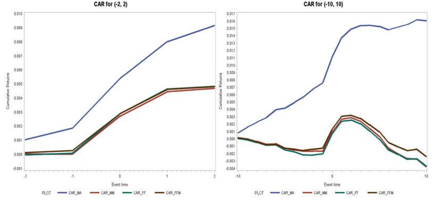
First, we present a graph of the failure rates of the firms in our sample in Figure 5. As the figure
shows, there is a substantial rate of failure for acquirers post-M&A in our sample. About one-third ofSustainability 2020, 12, 2999 17 of 31
firms fail within five years after the deal. Some studies find post-M&A failure rates of about 70% or
90% [3], so our estimates are relatively conservative. Such high rates of failure motivate an investigation
into the determinants of acquirer failure post-M&A. We, therefore, run a logistic regression with a
failure dummy as the dependent variable in Equation (12).
Pr(Failureit = 1) = f α + β1 ∗ tcit + β2 ∗ tcit 2 + γ0 Control variablesit + yt + ii (12)
where f(.) is the logit function.
Figure 5. Histogram comparing the number of deals that survive or fail post-M&A with various
time intervals. Source: Thomson Reuters Securities Data Company (SDC) Platinum Mergers and
Acquisitions database, Center for Research in Security Prices (CRSP) database.
The results are shown in Table 6 below. To aid interpretation, the marginal effects associated with
the regression are reported in Table 7, and the corresponding predictive margin graph and marginal
effect graph for two years post-deal are provided in Figure 6. The results in Tables 6 and 7 support
the due diligence hypothesis and the overdue hypothesis with respect to the likelihood of failure, as
predicted in hypotheses 2 and 4. The results are show a strong U-shaped relationship for the two- and
three-year time intervals. For the one-year and five-year intervals; however, the composite null of the
stringent test of a U-shaped relationship is not rejected. Overall, the results are shown in Tables 6
and 7 support the U-shaped relationship between time until deal completion and the likelihood of
failure. The predictive margins in Figure 6 conform to the shape of a logit distribution and reveal low
and decreasing levels of failure prediction before the turning point, and a sharp increase in failure
prediction in the days beyond the optimum, which worsens every day. Moreover, the marginal effect is
negative before the turning point, indicating that, before the turning point, each additional day reduces
the likelihood of failure (supporting the due diligence hypothesis), but that, after the turning point,
the marginal effect is always above zero, though it rises sharply and falls. However, the fact that it
remains positive beyond the turning point shows that each additional day beyond the turning point is
associated with an increased likelihood of failure, supporting the overdue hypothesis.You can also read