Prospects of application of mass-produced GNSS modules for solving high-precision navigation tasks
←
→
Page content transcription
If your browser does not render page correctly, please read the page content below
E3S Web of Conferences 244, 08006 (2021)                                 https://doi.org/10.1051/e3sconf/202124408006
EMMFT-2020

      Prospects of application of mass-produced
      GNSS modules for solving high-precision
      navigation tasks
      Vladimir Karetnikov1,*, Denis Milyakov2, Andrei Prokhorenkov1, and Evgeniy Ol’khovik1
      1Admiral  Makarov State University of Maritime and Inland Shipping 5/7, Dvinskaya str, Saint-
      Petersburg, Russia, 198035
      2Saint-Petersburg branch of Navis Inc, Russia

                    Abstract. Nowadays, both in the Russian Federation and in foreign
                    countries, the use of global navigation satellite systems (GNSS) for solving
                    various applied problems is an extremely popular solution. Taking into
                    account the current level of development of satellite radio navigation
                    systems, ordinary users have been able to determine their position with a
                    sufficiently high accuracy. However, some tasks require the use of high-
                    precision equipment of geodetic class. Such equipment allows obtaining
                    navigation solutions with an accuracy of better than 10 cm. Unfortunately,
                    the cost of navigation-class navigation equipment is extremely high.
                    Specialists working in the field of satellite navigation are particularly
                    interested in the possibility of using mass-produced GNSS modules to
                    obtain high-precision navigation solutions. In this paper, the possibility of
                    such an application will be considered, taking into account the results of
                    laboratory tests of a mass-produced navigation module.

      1 Introduction
          In accordance with the Federal Target Program “Maintenance, Development and Use of
      the GLONASS Global Navigation Satellite System for 2012-2020”, one of the most
      important tasks was the development of complementary GLONASS GNSS complexes,
      including the creation of systems for high-precision determination of navigation and
      ephemeris-time information. The area for the development of high-precision navigation
      systems based on GLONASS GNSS signals receives support not only in the field of public
      administration, but also in the commercial sector of the economy, which, given the negative
      foreign policy environment and sanctions, is an incentive for the creation of high-tech high-
      precision navigation equipment [1].
          Despite the fact that the development of the domestic market for the electronic industry
      and, as a consequence, high-tech navigation equipment lags behind Western companies,
      and many experts in the field of satellite navigation believe that it is not worth setting the
      goal of developing the GLONASS GNSS system to catch up with the developers of GNSS

      *   Corresponding author: karetnikovvv@gumrf.ru

© The Authors, published by EDP Sciences. This is an open access article distributed under the terms of the Creative Commons
Attribution License 4.0 (http://creativecommons.org/licenses/by/4.0/).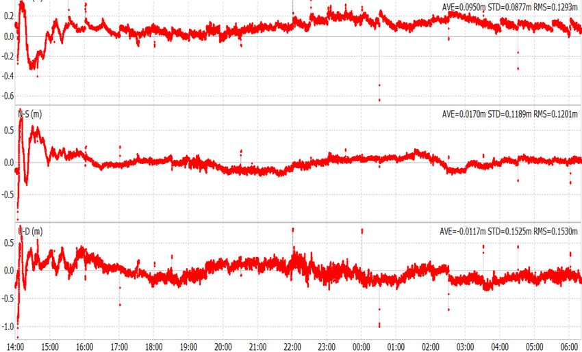
E3S Web of Conferences 244, 08006 (2021)                      https://doi.org/10.1051/e3sconf/202124408006
EMMFT-2020

      GPS in accuracy, since the current accuracy is enough for most tasks, the development of
      the fleet of high-precision navigation equipment in the Russian Federation continues [2].
          Determination of coordinates with a centimeter level of accuracy still requires the use of
      expensive GNSS consumer navigation equipment (CNE) [3]. However, at present, the basic
      elements of high-precision positioning technology using mass-produced GNSS modules
      have been developed and tested, which in the future, most likely, will make high-precision
      positioning available to almost any owner of a smartphone or, for example, an auto
      navigator. This will inevitably radically change the markets for geodesic and navigation
      equipment and geoinformation.

      2 Materials and Methods
      In 2019, KB NAVIS JSC developed a prototype of a set of high-precision navigation
      equipment (HPNE), operating according to GLONASS/GPS/GALILEO/BEIDOU GNSS
      signals, with the function of receiving assistive data via a radio channel. HPNE equipment
      performs high-precision positioning in absolute mode (PPP mode - Precise Point
      Positioning) [4,5] by joint processing of two-frequency measurements (pseudo-ranges and
      pseudophases) and high-precision ephemeris-time information (ETI) [6] of real-time GNSS
      in the form of RTCM 10403.2 standard coming from the Ministry of Defense Precision
      Navigation System (MD PNS).
          HPNE provides continuous tracking of GNSS GLONASS navigation spacecraft and
      conduct code and phase measurements by signals [7]:
          1. GLONASS:
          - high precision with frequency division: L1SF, L2SF;
          - high precision code division: L1SC, L2SC;
          - standard precision with frequency division: L1OF, L2OF;
          - standard precision code division: L1OC, L2OC, L3OC.
          2. GPS – L1 C/A, L1C, L2C, L5C;
          3. Galileo – E1bc, E5a, E5в;
          4. Beidou – B1I, B2I.
          The HPNE set includes:
          - navigation box with built-in rechargeable battery;
          - antenna unit;
          - charger;
          - a set of cables and accessories.
          Software developed to implement PPP mode in the prototype of HPNE provides:
          - determination of absolute coordinates, components of the velocity vector of the ground
      observer and corrections to the receiver time scale in real time (navigation mode);
          - processing of dual-frequency phase and code measurements of GNSS (IonoFree
      combinations) in real time using high-precision assistance information coming from the
      MD PNS (high-precision PPP determination mode);
          - registration of primary code and phase measurements with the purpose of subsequent
      transmission to the Center for Precision Information (CPI-M) of MD PNS (base station
      mode);
          - taking into account and correcting the main factors of observation errors, taking into
      account the recommendations of the IGS and the system for high-precision determination
      of ephemerid-time corrections (SHPD ETC).
          High-precision determination of coordinates in real time is carried out using modern
      algorithms for joint processing of GNSS signals and assistance information.

                                                   2
E3S Web of Conferences 244, 08006 (2021) https://doi.org/10.1051/e3sconf/202124408006
EMMFT-2020
3 Results
Solving coordinate-time tasks in PPP mode using assistance information.
The computational resources of HPNE (Dolomant's computing module operating at 600
MHz) make it possible to use recurrent navigation filters that estimate coordinates,
velocities and phase ambiguities, as well as tropospheric parameters (the wet component of
the vertical propagation delay of the navigation signal). The traditional approach to the
precision solution of the navigation problem for mobile equipment is the use of extended
Kalman filters (EKF) [8] and their various modifications.
As part of the work performed, a software multisystem PPP navigation algorithm based
on the Kalman filter was developed and implemented, which can be successfully used to
solve both static and dynamic problems of coordinate determination.
As an observation vector in such a filter, measurements of “ionospheric-free”
combinations of pseudo-ranges and phases are used [9]; the estimated parameters include
corrections to the coordinates, the receiver time scale, the values of phase ambiguities for
the used phase combinations, as well as the total vertical tropospheric delay or its wet part.
The inclusion of phase ambiguities in the estimated parameters makes it possible to use
the entire volume of available phase measurement information in their estimation, and not
only distance measurements of the corresponding channel, which makes it possible to
increase both the accuracy of the solution and the rate of its convergence. The downside is
the significant increase in computational costs caused by the increase in dimension.
The traditional algorithm includes two cyclically repeated main steps, commonly called
prediction and correction. Below, for an example, an algorithm for a single-system
implementation is given, corresponding to autonomous operation on the GLONASS GNSS
system:
Stage “Prediction”
X i+1 = ФX i . (1)
Pi+1 ФPi ФT + Q.
= (2)
Stage ‘Correction”
Pi +1H iТ+1
K i +1 = . (3)
H i +1Pi +1H iТ+1 + W
P=
i +1 Pi+1 − K i +1H i +1Pi+1. (4)
X i+1 + Ki +1 ( Ri +1 − R ( X i+1 ) ) .
X i +1 = (5)
Here the vector of observations:
R = col ( D1...DN , L1...LN ) , (6)
where Di – measurements of “ionosphere-free” combinations of pseudo-ranges and Li –
similar combinations of total phases.
Vector of estimated parameters:
X = col ( DX , DY , DZ , DT ,VT , N1...N N ) , (7)
3E3S Web of Conferences 244, 08006 (2021) https://doi.org/10.1051/e3sconf/202124408006
EMMFT-2020
Where DX, DY, DZ, DT – corrections to navigation coordinates and receiver scale, VT –
vertical tropospheric delay, or its wet part, N1…NN – values of phase multivalues for N
used satellites.
Matrix Ф defines the model of dynamics with model noise Q, P – the covariance matrix
of the estimate of the desired vector X, the observation noise is characterized by the matrix
W.
Н - gradient matrix:
H H H 1 M 0 … 0
x1 y1 z1 1
… … … … … … … …
H = H H H 1 M 0 . 0
xN yN xN N .
H H H 1 M 1 … 0
x1 y1 z1 1
… … … … … … … …
H H H 1 M 0 . 1
xN yN xN N .
Here Hx, Hy, Hz - direction cosines on satellites, Mi – values of the tropospheric display
function for the corresponding satellite.
In the case of an a priori unknown (stochastic) law of motion, as corrections to the
coordinates, it is advisable to seek corrections to the previously obtained conventional
navigation solution based on single observations. In this case, matrix Q will characterize the
coordinate noise of this navigation solution. Then the identity matrix can be used as matrix
Ф, except for the diagonal element corresponding to the estimate of the wet delay. I.e.:
−T
Ф = diag 1,1,1,1,exp emp ,1...1 (8)
Tcorr
where Темp – rate of data receipt and processing, Tcorr – the time constant of the
correlation of the errors of the “wet” part of the vertical tropospheric delay (usually selected
in the range of 1-3 hours).
In this case, the result of solving the traditional navigation problem is used as the
extrapolated DX, DY, DZ, DT. This scheme makes the EKF algorithm completely
independent of the consumer dynamics and the used model for predicting the coordinate
components of the vector of the estimated parameters. At the same time, such a scheme is
not optimal for many applications, since the use of more complex dynamic models for
extrapolation (with a corresponding expansion of the vector of estimated parameters due to
the corresponding derivatives of coordinates) or additional information from inertial
sensors will further narrow the filter tracking zone and increase the accuracy of the
assessment.
4 Discussion
To optimize the solution of the coordinate problem and accelerate the convergence, it is
important to correctly select the elements of the observation weights matrix W. It must be
recalculated dynamically and can take into account the change in measurement accuracy
depending on the signal-to-noise ratio, elevation angle, pre-smoothing time for distance
measurements (if used), and other factors. The traditional, simplest and most frequently
implemented approach involves the use of the value of functions of the elevation angle as
4E3S Web of Conferences 244, 08006 (2021) https://doi.org/10.1051/e3sconf/202124408006
EMMFT-2020
weighting coefficients. Correct formation of the weight matrix increases the rate of
convergence of the solution and increases its accuracy, especially in dynamic applications.
The following rule is usually used to form the weight matrix:
W diag (W1...WN ) , W
i (a) C02 , a a0 .
C02 sin 2 (a)
Wi (a) , a a0 .
sin 2 (a)
Here a – elevation angle of the observed i-th satellite. C02- nominal measurement noise,
angle a0 is chosen, as a rule, empirically.
The hardware implements two modes of PPP definitions - static [10, 11] and dynamic.
The main differences between static (used for static initialization) and dynamic algorithms
are as follows:
1. In the static algorithm, the corrections to the constant initial approximation of the
station coordinates are estimated, in the dynamic algorithm - to the results of the navigation
solution obtained from the measurements of pseudo-ranges.
2. In the static algorithm, the influence of lithospheric dynamics is removed from the
corrections (null-tide solution), in the dynamic one, this influence is kept.
3. Differences in the thresholds for rejecting faulty measurements (for statics, rejection
is more severe).
When processing the data, accounting and correction of the main error factors was
ensured, taking into account the recommendations of IGS and SHPD ETC:
- two-frequency combinations of phase measurements were used, which ensured the
elimination of the ionospheric error;
- high-precision ephemeris-time information of real time in the format of the RTCM
10403.2 (SSR) standard, coming from the Ministry of Defense precision navigation system
(MD PNS) and/or other similar sources, was used;
- the relativistic SRT and GRT corrections and the Wind-Up effect were taken into
account;
- to correct the hydrostatic part of the tropospheric delay, the Saastamoinen-Davis
troposphere model was used, taking into account the course of temperatures, humidity and
pressure according to the ICAO seasonal atmospheric model;
- when estimating the wet part of the tropospheric delay, the GMF display function was
used;
- for static problems, tidal phenomena in the lithosphere, caused by the influence of the
Sun and the Moon, as well as by the movements of the Earth's pole, were taken into
account and compensated for;
- additional control of undiagnosed disruptions of phase measurements (the main
method was control of the smoothness of the phase differences L1 and L2) and rejection of
gross errors (RAIM) were made.
Below are some of the HPNE test results, including those obtained on the models of the
equipment.
The values of the error (with a probability of 0.68) for determining coordinates in real
time in PPP mode and PPP mode with initialization when using the data of the assistance
information of the SHPD ETC or similar sources of high-precision ETI are given in Table 1
and Table 2.
5E3S Web of Conferences 244, 08006 (2021) https://doi.org/10.1051/e3sconf/202124408006
EMMFT-2020
Table 1. Values of the error (with a probability of 0.68) for determining the coordinates in real time
in the PPP mode when using the assistance information data (after the completion of the transient
process).
GNSS signal Error (with a probability of 0.68) in determining coordinates, m
reception mode х у H
GLONASS 0.14 0.12 0.26
GLONASS, GPS,
0.12 0.12 0.16
GALILEO, BEIDOU
Table 2. Error values (with a probability of 0.68) for determining coordinates in real time in PPP
mode with initialization when using the assistance information data (after completion of static
initialization).
GNSS signal Error (with a probability of 0.68) in determining coordinates, m
reception mode х у H
GLONASS 0.07 0.06 0.18
GLONASS, GPS,
0.06 0.06 0.10
GALILEO, BEIDOU
Below is shown the typical behavior of the HPNE coordinate solution during operation
and the results of processing absolute coordinate determinations in real time.
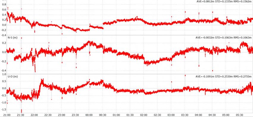
Fig. 1. Values of errors of positioning by GNSS GLONASS + GPS in PPP mode in real time.
Fig. 2. Values of errors of definitions by GNSS GLONASS in PPP mode in real time.
6E3S Web of Conferences 244, 08006 (2021) https://doi.org/10.1051/e3sconf/202124408006
EMMFT-2020
Conclusions based on the results of testing HPNE.
1. The Kalman filtering algorithms implemented in HPNE provide the solution of static
and dynamic problems of PPP-definitions, including those using measurements only by the
GLONASS system.
2. When working in real time, including only by GNSS GLONASS, the error values are
achieved at the level of 0.1 - 0.15 m in plain and 0.2 - 0.3 m in height.
3. When carrying out static initialization, the time of convergence of the navigation
solution in dynamics to a level of 10 cm with a discreteness of 1 sec is 0.6 - 1.0 hours.
5 Conclusion
The social effect of the introduction of high-precision positioning technologies with the
help of massively available consumer equipment is obvious in increasing labor productivity
in various fields of activity associated with the creation and use of geo-information.
Low-budget consumer equipment providing such a level of accuracy can be widely used
in solving various practical problems, namely:
- solving many problems of engineering geodesy;
- ensuring high-precision control of traffic and the development of unmanned vehicles;
- the use of automated control systems for equipment;
- control of dynamic deformations of technical structures;
- precise personal navigation (can be used, for example, when searching for small
inconspicuous or hidden under the ground, water or snow objects: underground or
underwater communications, wells, etc. - at industrial sites, railway stations, energy
facilities, utilities, etc.); and others.
References
1. V. Karetnikov, S. Rudykh, A. Ivanova, MATEC Web of Conferences 265, 02016
(2019)
2. V. Karetnikov, I. Pashchenko, V. Kozlov, A. Butsanets, IOP Conference Series:
Materials Science and Engineering 811, 012005 (2020)
3. V. Karetnikov, E. Ol’Khovik, A. Ivanova, A. Butsanets, Intelligent Systems and
Computing 1258 AISC, 421-432 (2021)
4. S. Savchuk, J. Cwiklak, A. Khoptar, Baltic Surveying 12, 39–43 (2020)
5. S. Bulbul, B. Bilgen, C. Inal, Measurement 171, 108780 (2021)
6. I.V. Bezmenov, Measurement Techniques 63(1), 7–14 (2020)
7. A. Karutin, Proceedings of the 33rd International Technical Meeting of the Satellite
Division of The Institute of Navigation (ION GNSS+ 2020) (2020)
8. A. Elmezayen, A. El-Rabbany, Survey Review, 1–15 (2020)
9. F. Basile, T. Moore, C. Hill, G. McGraw, Journal of Navigation 74(1), 5–23 (2020)
10. O. Sterle, B. Stopar, P. Pavlovčič Prešeren, Geodetski vestnik 58(03), 466–481 (2014)
11. M.A. Rabbou, A. El-Rabbany, Positioning 06(01), 1–6 (2015)
7You can also read