R 1334 - What drives investors to chase returns? by Jonathan Huntley, Valentina Michelangeli and Felix Reichling - Banca d'Italia
←
→
Page content transcription
If your browser does not render page correctly, please read the page content below
Temi di discussione
             (Working Papers)

             What drives investors to chase returns?

             by Jonathan Huntley, Valentina Michelangeli and Felix Reichling
April 2021

                                                                                   1334
                                                                          Number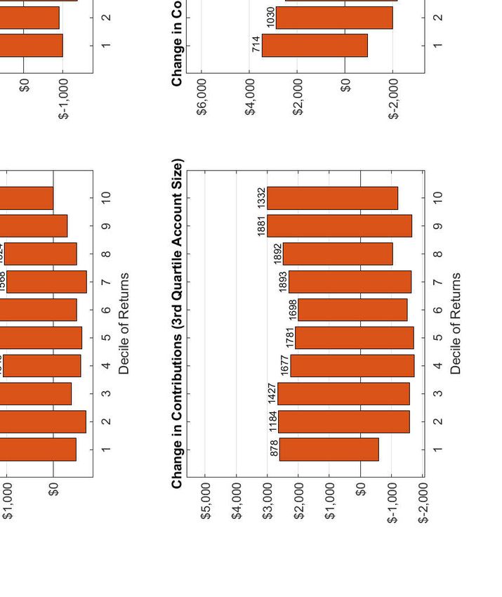
Temi di discussione
(Working Papers)

What drives investors to chase returns?

by Jonathan Huntley, Valentina Michelangeli and Felix Reichling

Number 1334 - April 2021
The papers published in the Temi di discussione series describe preliminary results and
are made available to the public to encourage discussion and elicit comments.
The views expressed in the articles are those of the authors and do not involve the
responsibility of the Bank.

Editorial Board: Federico Cingano, Marianna Riggi, Monica Andini, Audinga
Baltrunaite, Marco Bottone, Davide Delle Monache, Sara Formai, Francesco
Franceschi, Adriana Grasso, Salvatore Lo Bello, Juho Taneli Makinen, Luca
Metelli, Marco Savegnago.
Editorial Assistants: Alessandra Giammarco, Roberto Marano.

ISSN 1594-7939 (print)
ISSN 2281-3950 (online)
Printed by the Printing and Publishing Division of the Bank of Italy
WHAT DRIVES INVESTORS TO CHASE RETURNS?

                  by Jonathan Huntley*, Valentina Michelangeli§, and Felix Reichling*

                                                                 Abstract
       We use data on one-participant retirement savings plans to identify a behavioral bias in
savings decisions. Investors who earn top-decile returns increase contributions to their
accounts more than other investors. Accounting for the characteristics of the investors and of
their retirement savings accounts within a multivariate regression analysis, we first show that
such ‘return chasing’ behavior is robust to controls for financial illiteracy, macroeconomic
conditions, learning, transaction costs, housing prices, and informational frictions. We then
use a structural two-asset model with tax-deferred and taxable assets to show that a permanent
increase in expected returns produces investment responses for younger or liquidity-
constrained investors that are consistent with our data. Our results provide evidence that
younger investors' recent portfolio experiences have highly persistent effects on their
expectations.
JEL Classification: D14, G40.
Keywords: household finance, retirement saving, life-cycle.
DOI: 10.32057/0.TD.2021.1334

                                                                 Contents

1. Introduction ........................................................................................................................... 5
2. Data........................................................................................................................................ 9
   2.1 Administrative Data: Form 5500 .................................................................................... 9
   2.2 Filer Characteristics ...................................................................................................... 10
   2.3 Other Data: House Prices, Industry, and Employment................................................. 13
   2.4 Descriptive Evidence of Changes in Contributions...................................................... 13
3. Regression Analysis ............................................................................................................ 19
4. The Model ........................................................................................................................... 24
   4.1 Parameterization ........................................................................................................... 28
5. Simulation Results ............................................................................................................... 28
6. Conclusion ........................................................................................................................... 34
Appendix: Details on the Data ................................................................................................. 36
Appendix: Solution of the Model ............................................................................................. 39
Tables and figures .................................................................................................................... 41
References ................................................................................................................................ 54

_______________________________________
* Penn Wharton Budget Model, The Wharton School, University of Pennsylvania; § Bank of Italy, Economic
  Research and International Relations.
1 Introduction1
Do investors’ past experiences influence their investment decisions and expectations of returns in
a way that causes them to diverge from rational behavior? Many papers present evidence that
experiences do affect investment decisions in the form of “returns chasing,” where investors follow
price increases with additional investment.2 This bias is referred to as “chasing trends” and has
been used to explain the technology stock bubble of the late 1990s and early 2000s (Greenwood
and Nagel, 2009). Numerous empirical studies document returns-chasing in mutual fund choices
(Choi, Laibson and Madrian, 2010b). Some argue that “trend chasing” is tied to behavioral
biases (Bailey, Kumar and Ng, 2011). Choi et al. (2009) observe a positive correlation between
returns and contributions among participants in large-employer 401(k) plans and conclude that
returns chasing “indicate[s] that savings decisions are affected by random accidents of personal
financial history that should not matter to a rational agent.”Similarly, Bender et al. (2020) survey
higher-wealth investors, of whom 24 percent report that personal experiences in the stock market
are important for determining the equity share in their portfolios.3
In our work, we define returns chasing as the correlation between high returns in a finan-
cial account and additional investment in the same account, which we observe in Solo 401(k)
retirement accounts.4 Following similar work by Choi et al. (2009), we contribute to the existing
literature that seeks to identify the micro-foundations of returns chasing by exploring a dataset
1
This paper has not been subject to review by the Penn Wharton Budget Model. The analysis and conclusions
expressed herein are those of the authors and should not be interpreted as those of the Bank of Italy or the Penn
Wharton Budget Model.We would like to thank Alex Michaedelis, Efraim Berkovich, Francesco Columba, Paolo
Finaldi Russo, Daniel Kirsner, Jason Levine, Silvia Magri, Damien Moore, Sabrina Pastorelli, Richard Prisinzano,
Tarun Ramadorai, John Sabelhaus, Martino Tasso, the participants and discussants at several seminars, and two
referees for helpful discussions. We thanks Claire Sleigh and Shiqi Zheng for their excellent research assistance.
We also gratefully acknowledge the organizers of the CFP Board Academic Research Colloquium for Financial
Planning and Related Disciplines for awarding the 2019 TD Ameritrade Institutional Best Paper Award for
Behavioral Finance for an earlier version of this paper, which was titled “Chasing Investment Returns: Do
Learning, Literacy, and Experience Really Matter?”.
2
Many studies investigate circumstances in which returns chasing may be a rational behavior. In some model
frameworks, it is optimal for traders to follow the crowd anticipating that uninformed investors will subsequently
enter the market (De Long et al., 1990).
3
Similarly, personal economic experiences can shape macroeconomic expectations (Das, Kuhnen and Nagel,
2020).
4
In the literature cited above and many other studies, the term returns chasing is also used to describe similar
behaviors in portfolio allocation decisions.
5on retirement savings and by building a structural model. Using our data and model, we narrow
down a set of common explanations to one: an increase in expectations regarding future returns,
restricted to younger investors, explains the key empirical regularities we observe in our data.
We start with a list of causes that are commonly hypothesized to explain the returns chas-
ing we observe and that is documented by Choi et al. (2009): 1) financial literacy (Van Rooij,
Lusardi and Alessie, 2011); 2) information acquisition costs (Sims, 2003; Reis, 2006; Abel, Eberly
and Panageas, 2013; and Moscarini, 2004); 3) transaction costs (Kaplan and Violante, 2014); 4)
reinforcement learning (Choi et al., 2009; Kaustia and Knupfer, 2008; and Anagol, Balasubra-
maniam and Ramadorai, 2019); 5) experience (Greenwood and Nagel, 2009); and 6) changes in
expectations (Vissing-Jorgensen, 2003; Greenwood and Shleifer, 2014; Briggs et al., 2015; and
Gennaioli, Ma and Shleifer, 2016).5
We conclude that, among those hypotheses, changes in expectations limited to young in-
vestors are the best fit for the returns chasing behavior we observe in a publicly available ad-
ministrative dataset that contains information on 18 years worth of one-participant retirement
plans (also known as Solo 401(k) plans). This conclusion supports two important findings from
recent works on expectations formation: Experiences in early life have a much larger impact
than experiences later in life, and the impact of such experiences is permanent or highly per-
sistent (Malmendier and Nagel, 2011; Malmendier, Tate and Yan, 2011; Cronqvist and Siegel,
2015; and Malmendier and Nagel, 2015). We make six observations to support our conclusion
by documenting the stylized facts about these business owners, using regression analysis, and
simulating investor behavior in a buffer-stock type model (Carroll, 1997) with tax-deferred and
taxable assets (Gomes, Michaelides and Polkovnichenko, 2009; and Huntley and Michelangeli,
2014).
First, we observe that the investors in our sample self-identify as financially literate or em-
ploy financially sophisticated advisors because of the start-up costs associated with Solo 401(k)
accounts.6 Moreover, they tend to be more educated than the typical large-company 401(k) in-
5
There are many mechanisms through which expectations could be influenced. In addition to the mechanisms
discussed in the papers cited here, others cite overconfidence as a source of changes in expectations (Bailey, Kumar
and Ng, 2011) or the role of social interaction in disseminating information and changing expectations (Ambuehl
et al., 2018 and Duflo and Saez, 2003).
6
Establishing such accounts requires a significant degree of financial sophistication or the assistance of a
6vestor. Although households with less education are more likely to make errors than better edu-
cated households (Campbell, 2006), our highly educated investors—a huge fraction of whom are
doctors, lawyers, engineers, and other professionals with substantial educational requirements—
exhibit the same behavioral biases documented by Choi et al. (2009). This suggests that financial
literacy and education are not the proximate cause of returns chasing, a conclusion that fits with
previous research on the relationship between investment decisions and financial literacy (Choi,
Laibson and Madrian, 2010a; Choi, Laibson and Madrian, 2010b; and Lusardi and Mitchell,
2014).
Second, we observe that our agents actively manage their accounts by changing their con-
tributions each year. Less than 20 percent of contributors keep their contributions fixed at
nominal levels from one year to the next.7 Investors are free to make these changes because Solo
401(k) plans offer a wide variety of investment options with extremely low transaction costs.
Although there may be pecuniary and non-pecuniary transaction costs for making changes to
large-company 401(k) elections, these are not common to Solo 401(k) plans. Thus, this activity
likely reflects the plans’ low transaction costs, as well as the requirement that investors or their
advisors monitor their account at least once per year to file their tax returns and make contri-
bution decisions. Since investors are required to pay informational and transaction costs each
year, and we continue to observe returns chasing, we conclude that information and transaction
costs do not contribute to this behavioral bias.
Third, we find that returns chasing is concentrated among investors who realize top decile
returns.8 Indeed, investors in the top decile of annual returns typically contribute roughly 1.5
cents for each additional dollar of investment income, or almost three times as much as those
receiving average returns. This result is similar to that derived from experimental data (Kuhnen,
financial planning professional. For example, an E*TRADE individual 401(k) plan application is 20 pages long:
https://content.etrade.com/etrade/estation/pdf/Qualified_Retirement_Plan_App.pdf
7
Unlike large company plans, there is no easy way to elect contributions as a proportion of income. Solo
401(k) participants typically wait until the end of the year or tax-filing to elect a contribution denominated in
nominal dollars, which can be a function of cash-flow, earnings, expected income, liquidity needs, and other
factors.
8
We selected deciles because this was the level of disaggregation at which we could most clearly observe
returns chasing in the empirical distribution. Moreover, other studies (Barber, Odean and Zheng, 2005) document
returns chasing in financial flows into high performing mutual funds also break down their samples into deciles
for analysis.
72015). The fact that returns chasing behavior is concentrated asymmetrically among investors
earning top-decile returns suggests that reinforcement learning (Kaustia and Knupfer, 2008),
which more heavily weights personal experience, does not explain all of investors’ decisions in
the sample of Solo 401(k) investors.
Fourth, among those top-decile investors “chasing returns,” we observe a permanent (or
highly persistent) level shift in investors’ lifetime contribution profiles. When investors receive
top-decile returns, they increase their contributions for that and subsequent periods, a behavior
similar to the empirically observed long-term effects of personal experiences (Malmendier and
Nagel, 2011).
Fifth, the propensity to chase returns decreases with wealth and account age, which are
highly correlated with each other, which is a result consistent with other empirical studies (Choi
et al., 2009).
Sixth, in a structural, life-cycle, two-asset model with tax-deferred and taxable assets based
on those of Huntley and Michelangeli (2014) and Gomes, Michaelides and Polkovnichenko (2009),
only a permanent change in expectations (not a transitory one) can generate responses that
match key observations from our sample. The results of our simulations indicate that a per-
manent change in expectations can generate investment behavior for younger and liquidity-
constrained investors that is similar to that observed in the data—that is, a long-lived or perma-
nent shift in the level of tax-deferred contributions. However, temporary changes in expectations
fall short of explaining behavior for every subgroup of agents. A short-term increase in expected
returns leads to a drop in contributions in subsequent periods, as individuals revert to a contri-
bution profile similar to that of agents who did not experience exceptionally high returns.
In our model, permanent expectations generate responses similar to those we observe in the
data for agents who are more than a decade from retirement. Agents nearing retirement face
comparatively little lifetime idiosyncratic labor income risk and thus have less of a need to save in
their liquid account. When these agents expect a higher, permanent change to returns, they do
two things. First, they increase their contributions in a manner similar to younger agents. But
second, they also move a large fraction of their liquid assets into illiquid, tax-deferred accounts.
This behavior generates a large increase in tax-deferred contributions as they reallocate their
8savings, followed by a large decrease in tax-deferred contributions once they are done reallocating
their savings portfolio across taxable and tax-deferred accounts. Those older individuals still
permanently increase their tax-deferred contributions, but that increase is dwarfed by the effect
from asset reallocation, which we do not observe in the data.
The results from our simulation are aligned with the conclusions from a number of recent pa-
pers that provide empirical evidence that personal experience may result in permanent or highly
persistent changes in expectations, but that this effect is limited to younger or less experienced
investors. Malmendier and Nagel (2011) show how personal experiences have life-long effects on
investment patterns and risk taking, especially for young investors. Malmendier, Tate and Yan
(2011) show how early life experiences are correlated with CEOs’ investment decisions much later
in life.9 Malmendier and Nagel (2015) find that “young individuals update their expectations
more strongly than older individuals since recent experiences account for a greater share of their
accumulated lifetime history.” And Cronqvist and Siegel (2015) demonstrate that “Parenting
contributes to the variation in savings rates among younger individuals in our sample, but its
effect has decayed significantly for middle-aged and older individuals.” Finally, Giuliano and
Spilimbergo (2013) show that recessions have lifetime effects on political outlooks.
The remainder of the paper is structured as follows. In section II, we describe the data
sources and provide graphical evidence for investors’ changes in contributions. In section III,
we present the results of the regression analysis. In section IV, we introduce our model, and
we evaluate the simulation presented in section V. We offer conclusions and direction for future
work in section VI.
2 Data
2.1 Administrative Data: Form 5500
This section summarizes the main features of the Solo 401(k) defined contribution plans that
form our sample; a more detailed treatment of the plans and their differences from the typical
9
Similarly, Kuhnen and Miu (2017) document many instances when early-life experiences can affect decisions
among people with lower socioeconomic status.
9large-employer 401(k) is provided in Appendix 6.
The Employee Retirement Income Security Act of 1974 (ERISA) requires that retirement
plan sponsors—in this case, the individual filers and owners of the Solo 401(k) account—file
Form 5500 or one of its derivatives for a wide variety of retirement benefits.10 Starting from
these forms, we construct a dataset on single-employee businesses that sponsor their own defined
contribution plans. Each year from 1999 to 2017 contains some 15,000 to 20,000 records of these
Solo 401(k) accounts. We link individuals’ records across years using their employer identification
numbers (EIN) and the plan number, in the event that the filer maintains more than one Solo
401(k) account. Although a number of filers enter and drop out of the sample—depending on
whether or not their assets meet the filing threshold or they roll their assets into or out of other
retirement plans—we are able track many filers over several years.
For single-participant plans, the business owner or plan sponsor picks a plan administrator
(often him or herself) and a custodian (typically a bank or brokerage that holds the plan’s assets).
Most major brokerages provide custodial services and offer a suite of options covering potential
plan features such as loan availability, investment options, hardship withdrawal availability, plan
fees, and more. Plan sponsors can establish accounts with features important to them using any
of the major brokerages.
2.2 Filer Characteristics
Compared to investors in typical large-company 401(k) plans, investors in Solo 401(k) plans:
• are considerably more financially sophisticated or are more likely to directly employ a
financial advisor;
• are typically highly educated individuals, as shown in shown in Table 1;
10
The large majority of Form 5500 and 5500-SF filings are for businesses with multiple employees, ranging
from local businesses to large multinational conglomerates. Regardless, any business that sponsors a retirement
plan under ERISA is subject to the reporting requirement. For the defined contribution plans in our sample,
filers with Solo 401(k) accounts exceeding an aggregate value of $250,000 from 2007 on and $100,000 before 2007
are required to file. Many filers in our sample do not meet the filing threshold. These filers may have external
accounts that count toward the filing requirement; they may submit forms provided by organizations that service
the plans and are delivered nearly complete; or they may submit filings to minimize exposure to audits.
10• can select plan custodians to access low or no transaction costs;
• generally have higher contribution limits;11
• have access to a wide range of investment options;12
• pay any possible observation costs at least once per year, as they are required to file their
income tax returns and make contribution decisions.
Overall, 5500 filers have the option to contribute more than can be paid into traditional large-
employer 401(k) plans. They are generally allowed to make up to three types of contributions
to their Solo 401(k) accounts: a base amount (up to $18,000 in 2017); an employer contribution
of up to 20 percent of pre-contribution compensation, the sum of which cannot exceed the
inflation-indexed amount (up to $54,000 in 2017 before any applicable catch-up contribution);
and catch-up contributions for older filers ($6,000 in 2017).
Most plan sponsors make large contributions at the end of the year, or even in the subsequent
fiscal year, to optimize their cash flow and tax efficiency.13
Moreover, 5500 filers have the flexibility to choose from a larger choice set. Modal large-
employer 401(k) plan participants may be constrained by administrative processes as well as time
and pecuniary transaction costs, which may discourage them from updating savings decisions
when faced with income or wealth shocks. In contrast, 5500 filers and their advisors are already
familiar with these processes, which should make them no less likely to respond to wealth and
income shocks than modal large-employer plan participants.
11
Contribution limits for individual 401(k) plans were $55,000 in 2017 (or $61,000 for people age 50 and older),
considerably more than regular 401(k) participants are allowed to contribute ($18,000 plus employer’s match or
contribution in 2017, $24,000 plus an employer’s match or contribution for people 50 years of age and older). For
more details, see Internal Revenue Service Publication 560 at https://www.irs.gov/pub/irs-pdf/p560.pdf.
Large-employer plans have the option of setting the same high level of employer contribution limits, but rarely
do.
12
Personal retirement accounts can contain a huge variety of assets; however, there are several re-
strictions, mostly intended to arrest self-dealing behavior. See https://www.irs.gov/retirement-plans/
plan-participant-employee/retirement-topics-prohibited-transactions for some examples of disal-
lowed investments.
13
An informal survey of financial planning professionals attending the 2019 Certified Financial Planner Board
Academic Colloquium suggests that most Solo 401(k) account holders time their contributions with preparation
of their income and 5500 tax returns, which occur in the subsequent calendar year.
11Taken together, these requirements make Form 5500 and 5500-SF filers qualitatively different
investors from studied participating in large-employer 401(k) participants (Madrian and Shea,
2001; Agnew, Balduzzi and Sunden, 2003; Choi, Laibson and Madrian, 2004; and Choi et al.,
2009) or from more representative samples of households (Calvet, Campbell and Sodini, 2009).
Like most studies of retirement accounts, we are unable to observe filers’ entire portfolios.
And, unlike many of the investors contributing to large-employer 401(k) plans, investors in our
sample may have external, liquid assets on which they can draw when necessary.14 Nonethe-
less, the investors in our sample are likely to have higher personal income and, as a result,
high marginal ordinary income tax rates, which makes these tax-deferred accounts particularly
attractive.15
To focus on financial instruments that are (almost certainly) filers’ primary vehicles for
employer-based tax-deferred retirement savings, we restrict the dataset to active accounts, de-
fined as those for which the filer made a contribution in the current year or makes a contribution
in a future year. Many accounts in our sample may be inactive—they may still meet statu-
tory filing thresholds even though the business has been dissolved or suspended, or the account
has been superseded by an alternate tax-deferred instrument. When analyzing the empirical
distribution of the changes in contributions, we exclude the observations censored by statutory
maximums. We do include these observations in the regression analysis and specify a censored
regression to account for contribution limits.
We present descriptive account data in Table 2. The Form 5500 filers in our data have, on
average, more savings in these accounts than the typical U.S. household. The median household
actively contributing to an account in 2013 had a balance of $109,000, with an average balance
of $450,000 (see Table 2). By contrast, the median balance in 2013, as computed by Vanguard
and reported by the Center for Retirement Research (CRR) at Boston College, was $31,396; the
value for older individuals aged 55–64 was about $76,000.16 Over the sample period, median and
14
Most households that hold tax-deferred assets also hold some taxable assets as well. For example, in the
2001 Survey of Consumer Finances, Huntley and Michelangeli (2014) find that about 65 percent of households
have tax-deferred assets, and of those, 86 percent have both tax-deferred and taxable assets.
15
Phaseouts for exemptions, deductions, and credits may make the effective marginal tax rate on labor income
even higher than the statutory rates for each income bracket for high-income filers.
16
The Vanguard/CRR report is available at http://crr.bc.edu/wp-content/uploads/2017/10/IB1 7 − 18.pdf
12mean values of the accounts for holders who have taken a distribution are typically considerably
larger than the mean and median of accounts whose holders have made a contribution.
2.3 Other Data: House Prices, Industry, and Employment
The data from Form 5500 and Form 5500-SF can be matched with indicators from other sources
to control for the effects of changes in real estate prices and in local economic conditions.17
Kuchler and Zafar (2019) find that changes in local house prices affect investors’ perceptions of
other macroeconomic variables. Therefore, we pair the sponsor’s business zip code with data on
house prices from Zillow and include it in our analysis.18
Forms 5500 and 5500-SF do not contain data on labor income. However, the plan sponsor
provides a six-digit NAICS industry code for the business, which, combined with the zip code,
allows us to use to pair each observation with industry- and county-specific information from
County Business Patterns (CBP).19 The CBP dataset provides employment and payroll statistics
at both the countywide and industry-specific level and uses the same NAICS codes reported in
Form 5500 filings. We match employment statistics’ two- and four-digit NAICS classifications.20
2.4 Descriptive Evidence of Changes in Contributions
To document how investors use their Solo 401(k) accounts, we start by showing (in Table 3)
changes in account contributions from one year to another for filers with active accounts whose
The authors note that the Survey of Consumer Finances shows increasing values for 401(k) balances for older
participants, but still well below the median of our filers.
17
Unlike employees of larger business, self-employed business owners may be able to sell their businesses.
Therefore, to the extent that local economic conditions affect the value of the business, they may have a significant
effect on the plan sponsors’ savings decisions.
18
Zillow maintains a dataset of median house prices for single family homes by zip code, which is available
back to the beginning of our Form 5500 dataset for the majority of the zip codes in our sample. Zillow data is
available at https://www.zillow.com/research/data/.
19
CBP data is available at https://www.census.gov/programs-surveys/cbp/data/datasets.html.
20
The 2017 NAICS manual describing the classification system is available at https://www.census.gov/eos/
www/naics/2017NAICS/2017_NAICS_Manual.pdf. We match the NAICS level across the Form 5500 filings and
the CBP at the least granular (one digit) to most granular (six digit) classification. We find, however, that
percent change in the indicators at the five- and six-digit NAICS levels is exceptionally noisy, especially for small
industries and in small counties. Therefore, our analysis is based on four- and two- digit industry categories.
13contributions were not constrained by statutory limits.21
In our sample, plan sponsors make frequent changes to their annual contributions, and some
of those changes are quite substantial. One reason for this behavior is that, unlike participants
in large-employer 401(k) plans, these investors may not be able to compute income at short
enough intervals to serve as a metric on which to base regular contributions. Over most years,
even if the median change in contributions is zero, around 80 percent of filers make a change
to their annual contributions. Of those modifying their contributions, approximately half make
fairly modest changes, in a range of $2,000 around the median. The remaining investors make
much larger changes to their contributions: Typically just over a quarter of filers make changes
in excess of $5,000 in a given year.
There is some evidence of time-varying effects on moments of account contributions, similar
to the effects observed by Guiso, Sapienza and Zingales 2018. The distribution is shifted toward
negative changes during the 2008 and 2009 recession compared to 2007 and 2010, the years that
bookend the recession. The 25th percentile in 2008 is more than $1,000 lower than in 2007
and 2010. The 75th percentile in 2008 is about $800 lower than 2007, and $900 lower than in
2011. In years outside the recessions, the percentiles appear remarkably alike: For example, the
percentiles in 2013 are quite similar to the percentiles in 2005.
All of this activity points to accounts that are actively managed, which raises the likelihood
that these accounts will reflect marginal changes to investors’ savings. The accounts in this
sample are rarely put on autopilot, as is typical for large-employer 401(k) participants (Madrian
and Shea, 2001)). This leads to a much greater degree of overall variation (shown in Table 3)
than is observed in studies of traditional 401(k) participants (Choi et al., 2009 and Madrian and
Shea, 2001).
We present a visualization of the empirical distribution of dollar changes in contributions
in active accounts in Figure 1. Specifically, the bars show the middle 50 percent (middle two
21
Filers who report inactive accounts—defined as accounts that are specified as closed on the Form 5500 or
inferred as closed from a lack of subsequent contributions in any future filings—may have closed the business,
retired, or may be making contributions to other accounts. In all of these cases, the lack of contributions may
not reflect the filers’ savings decisions. Of the approximately 150,000 observations of changes in contributions,
about 135,000 were unconstrained by the annual maximum contribution limit ($54,000 in 2017, plus potential
catch-up contribution) in both the current and previous years.
14quartiles) of filers sorted by decile of returns. We compute each account’s annual return by
taking 401(k) income, which is directly reported in dollars on Form 5500, and dividing it by
the beginning-of-year balance. For all subsequent empirical analysis, we discard two additional
types of observations: investors who rolled over external funds into the account and investors
whose beginning-of-year account value was zero. In the former case, we do not know the date
on which the rollover occurred, and since some of the rollovers are quite large, our computed
return will likely be quite inaccurate. In the latter case, investors likely established the account
during the year, which presents similar challenges.22
If all contributions were made on December 31, the basis will equal the beginning-of-year
balance in the account. If the contributions were made significantly in advance of the end of
the calendar year, computed returns will incorporate income from these mid-year contributions.
Although contributions almost always come at the very end of the year, or in the subsequent
calendar year before Form 5500 is filed, it is possible that large and increasing contributions
made early in the year could select some investors into higher deciles.23 For robustness, we try a
regression analysis that adjusts the basis on which 401(k) returns are calculated using a fraction
of the plan year contributions. Although the estimates change slightly, the qualitative results
remain the same.
The number above each bar is the number of observations in the decile; the bar thus represents
the range of the middle half of those observations.24 The left bar (about -$800 to $2,200)
represents the middle half of the range of changes for investors who earned returns in the lowest
decile of the sample in each year. The next bar (about -$1,000 to $2,200) is the middle half of
changes to contributions for investors who realized returns in the second decile in that year. Most
22
Accounts must be established by the end of the calendar year, and may be seeded with a contribution in
advance of actual contribution deadlines.
23
Based on informal conversations with professionals and practitioners at the Certified Financial Planners 2019
Academic Research Colloquium, nearly all contributions come at the end of the year or in the subsequent year.
According to literature from the New Direction Trust Company and other sources, the employee contribution is
due on December 31st; however, employer profit-sharing contributions to Solo 401(k) accounts are due no later
than the time the tax return is due.
24
We compute the thresholds for the deciles of returns from all investors filing a return for that year. To com-
pute the change in contributions, we also need to observe the same plan in the previous year. As a consequence,
there is some variation in the number of observations used to construct the empirical distribution by decile of
returns.
15bars span a range of about $3,000, which indicates that about half of the filers make changes in
a $3,000 range located asymmetrically around zero.25
The filers in the top decile of returns for each year show changes to their contributions that
are qualitatively and quantitatively different from those of investors who earned lower returns.
Specifically, we find that the 75th percentile is associated with contributions higher by about
$1,000 or slightly more compared to the 75th percentile of the nine decile of returns; the bottom
25th percentile exceeds by about $800 the average of the rest of the deciles of returns. This
represents a substantial shift in behavior for investors earning exceptional returns and suggests
that a fraction of the population earning returns in the top decile may be chasing returns.
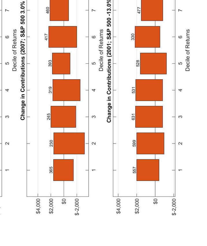
To evaluate whether returns chasing depends on macroeconomic conditions, we present in-
vestors’ behavior in three years representative of different financial market conditions—2001,
2007, and 2017—in Figure 2. In spite of the greater variance in the range of these smaller sam-
ples’ middle 50 percent, these three years illustrate that investors in the top decile appear to
contribute more than their contemporaries regardless of actual returns in a specific year.
In 2017, the S&P 500 increased by a healthy 19.4 percent, and investors who realized returns
in the top decile increased their contributions substantially more than investors in any other
decile, as shown in the top panel. By contrast, 2007 generated much more modest returns in
equities markets. In this year the S&P 500 had a return of about three percent. Nonetheless,
the middle panel illustrates that investors in the top decile continue to show the same behavior,
with the 75th percentile contributing nearly $2,000 more than investors in the other nine deciles.
In 2001, when the S&P 500 lost about 13 percent of its value, investors needed to earn only six
percent to get to the top decile of returns. As shown in the bottom panel, investors at the 75th
percentile in the top decile still increase their contributions by about $600–$700 more than their
peers in each of the other nine deciles of returns. In all three of these cases, investors earning
top-decile returns appear to be chasing returns. This indicates that the relationship between top
returns and contributions is common to all types of aggregate conditions in equities markets.
We evaluate changes in contributions against returns by account age. The results are similar
25
Although not shown, there is typically a significant mass of about 15 percent of the population exactly at
zero, consistent with what was reported in Table 3.
16to the changes in contributions evaluated by changes in account size, probably because the two
variables are highly correlated, especially in retirement accounts. A 5500 filer is not required to
divulge the plan sponsor’s age; however, the sponsor does provide the date on which the account
was established, which is highly correlated with both the age of the account holder and the
account holder’s investing experience.
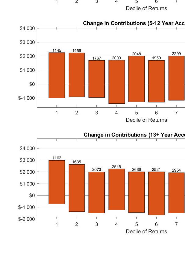
Figure 3 has three panels with sub-samples sorted by account age. The ranges for the
account age are selected so that each sub-sample represents approximately one-third of the
entire population of filers. The upper panel shows accounts that have existed for four or fewer
years; the middle panel contains accounts open between five and 12 years; and the bottom
panel contains accounts open for more than 12 years. All panels indicate that investors earning
top returns choose to make some additional contributions in tax-deferred accounts. In the top
panel, we show a $1,500 higher 75th percentile contribution for the top decile of returns relative
to the ninth decile. Similarly, in the middle panel, investors in the top decile of returns make
contributions higher by about $1,000 than those receiving returns in the lower deciles. In the
bottom panel, the account holders (who are among the most experienced investors in the sample)
also appear to chase returns, but to a lesser degree than their younger counterparts. The 75th
percentile of contributions for investors with returns in the top decile is higher than it is for
investors in most of the middle deciles. Nonetheless, the distribution of contribution increases
is similar among the top and bottom deciles.
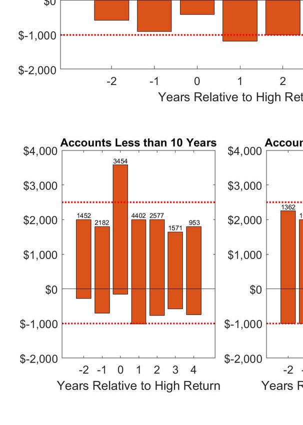
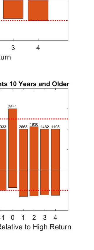
In Figure 4, we take a deeper look at the effects of prior top decile returns on the distribution
of leading and lagging contributions. The dashed lines define the middle two quartiles for the
entire distribution. Each bar shows the change in contributions for investors who earned returns
in the top decile at different time horizons. For example, the first bar shows the change in
contributions for investors who earned returns in the top decile two years after this contribution,
and the far right bar shows the middle two quartiles of changes in contributions for investors
who earned returns in the top decile four years earlier than the contribution. From the top
panel of this figure, which includes all Form 5500 filers, we can identify two clear features of the
dataset. First, on average, investors increase their contributions in the plan year during which
they make returns in the top decile. The 75th percentile is about $1,300 higher for those two
17periods than it is for any other periods represented in this graph. The 25th percentile is also
a few hundred dollars higher than the threshold for the bottom quartile for any of the other
periods represented in this graph. Second, some fraction of the investors earning high returns
appear to permanently shift the level at which they make those contributions. Indeed, the figure
shows a strong contemporaneous correlation between high returns and changes in contribution,
but there is no offsetting decline that would indicate that these investors return to their previous
level of savings in subsequent periods.
In the bottom two panels, we show the same results conditioned on account age. In the
bottom left panel, we show the middle two quartiles of changes to contributions for accounts
that have been open for fewer than 10 years. In this case, the effect is quite strong; the 75th
percentile in the year of the high return is about $1,700 higher than it is in any other year, and
the 25th percentile is slightly higher than the preceding and subsequent years. As for the upper
panel, this suggests that some investors significantly increase their contributions, and maintain
their contributions at this higher level. By contrast, in the bottom right panel, we show the
middle two quartiles of changes to contributions for accounts that have been open for a decade
or longer. In this case, the 75th percentile of changes in contributions in the same plan year as
top-decile returns are higher than the adjoining years by about $1,000, but still only about $500
higher than the entire sample’s 75th percentile, denoted by the horizontal dashed line. These two
bottom panels show that the relationship between top-decile returns and changes with investing
experience, reflecting the empirical distribution seen in Figure 3.
In the next section, we attempt to quantify the effects of high returns by estimating a censored
regression model. After that, we develop our two-asset, life-cycle model with taxable and tax-
deferred assets to evaluate conditions under which changes in expectations can be reconciled
with these qualitative and quantitative observations.26
26
Additional analysis of the empirical distribution of changes to contributions conditional on account size is
available in Appendix 6.
183 Regression Analysis
We use the preceding graphs to motivate our regression analyses, which we use to quantify the
relationship between returns and contributions. As before, the observations are drawn from ac-
tive accounts, defined as those into which the sponsor makes contributions contemporaneously
or in the future. Contemporaneous or future activity is a good indicator that the account is
accessible for additional contributions (as opposed to inaccessible due to changing jobs, clos-
ing the business, or retiring). Overall, the results from our regressions mirror the trends and
observations shown in the figures.
Our specification accounts for the possibility that filers’ contributions may be censored—that
is, equal to the maximum employee plus employer contributions allowed by law.27 We consider
several specifications and include a set of controls, such as employment changes at the two- and
four-digit NAICS level, both at the county and the national level, and employment changes for
the entire county over all industries.28
We estimate the following system:
27
There is a maximum employee deferred compensation component to the contribution and maximum employer
profit sharing component to the savings. In 2015, the deferred compensation component is $18,000. In 2015,
the “profit sharing” component is 20 percent of pre-contribution income, up to $35,000. For an individual over
the age of 50, there is an additional employee “catch-up” contribution allowed. In 2015, the maximum allowable
catch-up contribution was $6,000. If the filer is at the deferred compensation and profit sharing maximum for
his or her contribution—equal to $53,000 in 2015, for example—we assume that the observation is censored. If
the filer is above that threshold, but below the threshold plus the catch-up contribution ($59,000 in 2015), we
assume that the observation is uncensored. If the filer claims contributions equal to the deferred compensation,
profit sharing, and catch-up combined—$59,000 in 2015—we assume that the filer is censored. If the filer is above
all three, we assume that the filer either made an error or followed the contribution with a recharacterization,
either of which necessitates discarding the observation. The actual limit to contributing to the account may be
lower than the $53,000 in 2015; however, the majority of contributions below that limit are small enough that
the contribution limits based on income almost certainly do not apply. Moreover, as shown in Table 1, the vast
majority of businesses in the sample employ high-income professionals.
28
We run a number of specifications using countywide and industry-specific tax return data from the Statistics
of Income (SOI) and and found nearly identical results. We use changes in aggregate wages and salaries to measure
the economic growth at a county level, and aggregate wages from the business SOI data at the national level with
industries matched at the most granular NAICS classification available. The regression results using variables
drawn from the SOI for businesses and households are sometimes statistically significant but rarely economically
significant. Lastly, we try a number of different specifications involving different combinations of county and
industry employment data and found nearly identical results.
19
0 if Π(i, t) ≤ 0
Ci,t = Π(i, t) if 0 < Π(i, t) < mi,t (1)
m
if Π(i, t) > mi,t
where
Π(i, t) = α0 + α1 Wi,t + α2 Ei,t + α3 Xi,t + α4 Ci,t−1 + ǫi,t (2)
The variable Ci,t is the contribution made by investor i at time t. Contributions are bounded
below by 0 and above by mi,t , which we set to the statutory employer plus employee limit, ad-
justed by the catch-up contribution limit if the level of contributions indicates that the individual
is eligible to make a catch-up contribution.29
The vector Wi,t is populated with the variables related to wealth: the dollar change in the
median house price for the same zip code as the investor, the investment income in dollars, and
interactions with other indicators.30 Investment income comes directly from Form 5500.31 Given
the typical size of these accounts, investment income can be quite substantial.
To quantify the effect of high returns on contributions illustrated in Figure 1, we include
interaction variables in Wi,t . We specify an indicator that is equal to one if the returns are in
the top 10 percent of all returns from that year, and zero otherwise. As shown in Figure 1,
the propensity to contribute increases when returns are high; this interaction term quantifies
that relationship. In various specifications, we interact the high returns indicator, the lagged
high returns indicator, and a low returns indicator with investment income. We also interact
the investment income with the age of the account and the natural log of the beginning-of-year
29
We included all observations for which the investor made contributions above the non-age-adjusted maxima
but below or equal to the age-adjusted maxima. Even if the filer made a mistake and contributed a catch-up
contribution, this decision still reflects their savings decision. The vast majority of individuals in this range are
at the age-adjusted maxima.
30
We specify our dependent variable (contributions) and investment income in dollars. Choi et al. (2009) use
percent returns as a regressor and contributions as a share of income as the dependent variable. We do not have
income, so this specification is unavailable to us. We considered other specifications such as natural logs, however,
using levels in dollars was most consistent with the censored regression specification, accommodated a sample in
which a sizable percentage contributed zero dollars, and has an straightforward economic interpretation.
31
Participant loans are not included in income; following Form 5500, participant loans are treated as an asset.
Therefore, obtaining a loan would not affect our measure of income.
20value of the account to see whether any relationship abates with experience.
In addition to changes in asset values, we include a number of variables that may characterize
potential health of the business, summarized by the vector Ei,t . This vector includes percent
changes in employment in the entire county. It also includes changes in employment in the
filers’ industry at a county and a national level. Finally, the vector Xi,t includes time-dummy
variables. We removed the top and bottom one percent of observations sorted by income.32
Clustering was applied at the county level; we applied clustering at the state level and found
only small differences in the standard errors.
We present the main results in Table 4.33 The first column shows the baseline specification
containing no interaction variables, and is closest to the analysis presented by Choi et al. 2009.34
The coefficient on investment income is positive and significant; on average, for every dollar of
returns, contributions to the account increase by about 0.8 cents. These coefficients may seem
small; however, they are applied to large regressors. Some investors make very large returns
in dollar terms, which are correlated with significant changes in total contributions. Moreover,
since there is a good deal of persistence in these savings decisions, even moderate changes in
savings decisions early in life can have very large effects on the size of investors’ savings at
retirement. For example, an investment income of $50,000 correlates with a $400 increase in
yearly saving, leading to a change in behavior that could result in tens of thousands of dollars
in additional savings at retirement.
Several local employment or industry-specific employment indicators are correlated with
changes in contributions. Change in employment at the county level has a small effect on con-
tributions: A one-percent change in this variable leads to about a $33 increase in contributions,
32
In many of these cases, the income from these assets listed on Form 5500 likely does not reflect actual
year-to-year changes in the market value of the investment.
33
We excluded the top and bottom one percent of observations by total investment income. In many cases,
these incomes were extraordinarily unlikely to represent actual income generated by their assets. In some cases,
these numbers were the result of filing errors or other behavior that did not reflect or underlie any deliberate
life-cycle savings decisions.
34
All specifications include the following controls: constants, year dummies, change in employment for the
filers’ industry classification at the county level by two- and four-digit NAICS codes, change in employment for
the filers’ industry classification at the national level for the two- and four-digit NAICS codes, and change in
total county employment. Clustering is applied at the county level; applying clustering at the state level does
not materially change the results. For brevity, we omit reporting some variables that do not have statistically
significant effects.
21which is significant at the 10-percent level. A one-percent change in the two-digit NAICS em-
ployment category at the national level leads to an increase in contributions of about $106. The
coefficient on lagged contributions is about 0.943, which indicates that the increased contribu-
tions from a high-return year persist for several years.
All time dummies are included in the regressions, but we limit reporting to years around the
two recessions in our sample. The coefficients on these dummies indicate that there is a fairly
sharp change in behavior at the onset of recovery. The coefficient jumps by nearly $3,000 from
2001 and 2002 to 2003, a result that is common to all regression specifications. Nonetheless,
after 2003, the year dummy returns to levels that are stable between 2005 and 2008. By contrast,
between 2008 and 2010, the coefficient drops by about $800 to $900, and remains statistically
indistinguishable from zero in every subsequent year through 2016.
In the second column on Table 4, we interact investment income in dollars with a dummy
variable indicating that the investor earned contemporaneous top-decile returns. This specifica-
tion admits the possibility that the effect of returns on contributions is non-linear, and is meant
to allow for the possibility that investors who realize top returns have qualitatively different be-
havior, as shown by Figure 1. The coefficient on the indicator indicates that higher contributions
among the filers with higher returns explains a large fraction of the effect of higher returns. A
dollar of additional investment income is correlated with 0.6 cents of additional contributions to
Solo 401(k) accounts. Investors in the top decile of returns contribute an additional 0.9 cents
for each additional dollar of investment income, for a total of about 1.5 cents for each addi-
tional dollar of income. The other covariates remain similar in both magnitude and statistical
significance.
The third column of Table 4 shows the same specification, but with the interaction of prior-
year, top-decile returns. If investors are learning, we would expect the effects of high returns on
investor behavior would begin to dissipate in subsequent years. Although a point estimate of
the coefficient is slightly negative, we are unable to reject the null hypothesis that the coefficient
is zero. This result is consistent with the investor behavior over time documented in Figure 4.
Moreover, the coefficient on lagged contributions is close to one, which confirms the observation
from Figure 4 that investors receiving high returns shift their levels of contributions. All other
22coefficients are similar to their values in the second column.
We try several specifications to determine how age, wealth, low returns, and house prices in-
teract with investor behavior, and report the results in Table 5. The coefficients and significance
of all geography-specific indicators and time dummies are extremely similar to their analogues
in Table 4, and so we do not report them. In the first column, we introduce the dollar change
in the median single family house price as a regressor. For every dollar increase in median
single-family house price in the same zip code, investors increase their contributions by about
0.5 cents; however, we fail to reject the hypothesis that this coefficient is zero. The remaining
coefficients are extremely similar to all of the specifications reported in Table 4: A dollar of in-
come tends to increase contributions by about 0.6 cents, but having a top-decile return increases
the contribution to about 1.5 cents for each additional dollar of income.
In the second column in Table 5, we interact the natural log of the account size with in-
vestment income and a high returns indicator. This will allow us to see whether the propensity
to chase returns diminishes with account size. We see a clear negative correlation between the
natural log account size and contributions. This indicates that the effect is quite strong for
investors with small accounts, and abates as their accounts grow.35 Specifically, if the account
size roughly doubles (the log value increases by one), the estimates suggest that investors in the
top decile reduce their contributions per dollar of investment income by about 0.5 cents.
In the third column, we add account age, which we interact with high returns and investment
income. We find that account age, which is correlated with investor age, has a negative sign
significant at the five percent level. For the investor with a brand new account, high returns
are correlated with a 2.3 cent increase in contributions for each dollar of income, a relationship
that abates at a rate of 0.06 cents for every additional year that the account is open.36 This
finding is similar to what we observe in Figures 3 and 4, both of which seem to indicate that the
propensity to chase returns is lower for more experienced investors.
In the fourth column, we evaluate a specification with low returns to see whether investors
35
We also tried specifications where we broke the sample into tertiles or quartiles by account size, but we did
not identify any statistically significant coefficients on the account size indicators among these specifications.
36
We tried specifications with both account size and account age; those variables are highly correlated. Al-
though we saw the expected signs in each case, there was no statistical significance attached to either coefficient
individually.
23You can also read