Reading Guide for Capacity Calculation & Market Coupling KPIs

Reading Guide for Capacity Calculation &
Market Coupling KPIs

Version 1.0
Date 11-03-2021
Status Draft Final

Document creation and distribution
Document Owner CCR Core CC & MC KPI TF, Core FB MC A & FBV TF
Function
File location
Distribution

Approval
Version Date Name Function Signature

Previous versions
Version Date Author Summary of changes

Related documents

Attachments

Reading Guide for Capacity Calculation & Market Coupling KPIs

Contents

 1 Introduction................................................................................ 3

 2 KPIs ........................................................................................... 3
 2.1. Introduction .................................................................................... 3
 2.2. Adjustment for minimum RAM and LTA inclusion .................................. 4
 2.2.1. KPI 1 - Average maximum AMR per CNE per BD (Top 10) ........... 4
 2.2.2. KPI 2 - Average maximum AMR per TSO per BD ........................ 5
 2.2.3. KPI 3 - Average maximum AMR+LTAmargin per CNE per BD (Top
 10) .......................................................................................... 6
 2.2.4. KPI 4 - Average maximum AMR+LTAmargin per TSO per BD ....... 7
 2.3. TSOs’ adjustment after validation ....................................................... 8
 2.3.1. KPI 5 - Share of timestamps with intervention per TSO .............. 8
 2.3.2. KPI 6 - Total IVA applied per MTU for each CNE affected by TSO
 intervention .................................................................................... 9
 2.4. Market Impact Assessment (MIA) ..................................................... 10
 2.4.1. KPI 7 - Most often presolved CNEs (Top 20) ........................... 10
 2.4.2. KPI 8 - Most limiting CNEs (Top 20) ....................................... 12
 2.4.3. KPI 9 - Clearing prices, price spread and price convergence ...... 13
 2.4.4. KPI - 10 CNECs with non-zero shadow price per timestamp ...... 14
 2.4.5. KPI 11 - Core Social Welfare ................................................. 15
 2.3.6 KPI 12 - Paradoxically Rejected Block Orders (PRB) ................. 16
 2.5. Power System Impact Analysis (PSIA) .............................................. 17
 2.5.1. KPI 13 - Min and Max Net Positions per bidding zone ............... 17
 2.5.2. KPI 14 - Highest virtual margins at MCP per TSO, per BD ......... 18
 2.5.3. KPI 15 - RAM before and after RAO per TSO ........................... 20
 2.5.4. KPI 16 - Average sensitivity of RAs per TSO............................ 20
 2.5.5. KPI 17 - Non-Core exchanges & flow deviation on non-Core bidding
 zone borders ................................................................................. 21

Version – Date 11-03-2021 Page 2 of 23

Reading Guide for Capacity Calculation & Market Coupling KPIs

1 Introduction
According to Article 28(4) of the Day-ahead Capacity Calculation Methodology (DA CCM),
Core TSOs have the obligation to continuously monitor the effects and the performance of the
application of this methodology during the internal and external parallel runs. For this purpose,
TSOs have developed a set of Key Performance Indicators (KPIs), which was endorsed by Core
NRAs. Core TSOs will publish this set of KPIs jointly with NEMOs in a report on a monthly
basis on JAO.
The document at hand aims at introducing the reader solely to the calculated Capacity
Calculation (CC) and Market Coupling (MC) KPIs. It is not intended to be a general
introduction to Core Flow-Based Market Coupling (FBMC). The Core Consultative Group
(CCG) meeting on the 7th of October 2020 provided a more thorough overview on the latter,
which can be accessed via a presentation and a recording of the meeting.

2 KPIs
2.1. Introduction

The rationale behind the different KPIs and categories is to provide data and insights on the
different steps along the day-ahead CC and MC process. The picture below gives an overview
on the different steps and associated KPIs.

Source: Adaptation of CCG presentation slide 12 (7th of October 2020)

Version – Date 11-03-2021 Page 3 of 23

Reading Guide for Capacity Calculation & Market Coupling KPIs

 2.2. Adjustment for minimum RAM and LTA inclusion

 2.2.1. KPI 1 - Average maximum AMR per CNE per
 BD (Top 10)

Short Name of KPI KPI 1 - Average maximum AMR per CNE per BD (Top 10)
Article DA CCM Article 17. Adjustment for minimum RAM
Granularity Per Business Day
Aggregation Over all CNECs and all timestamps

KPI Description
KPI 1 analyses the adjustment for the minimum remaining available margin (AMR) applied by each TSO on each CNE, i.e.
the exclusive effect of the minimum RAM factor (Ramr, see Article 17 (9) DA CCM).The difference between Ramr and the
absolute minRAM for Core. The Ramr constitutes the total of all market exchanges, both Core exchanges and non-Core
exchanges (Fuaf). The minRAM for core = max (20%*Fmax, Ramr*Fmax – Fuaf, 0). Hence, this KPI needs to be read in
conjunction with the Ramr applied by each TSO, which are published on JAO.
Interpretation key: The higher the KPI, the higher the amount of virtual capacity that is to be added to the “natural” level of
the remaining available margin (RAM) present in the CGM in order to reach the Ramr.
KPI 1 is calculated as the Average Maximum AMR value in MW per BD (KPI 1a) and also as a percentage of the maximum
admissible power flow Fmax (KPI 1b). In this KPI only CNEs with AMR > 0 are taken into consideration but timestamps
(TS) with AMR = 0 are included in the calculation. As CNEs have Contingencies associated with them (CNEC), the values
of the KPI are obtained by first calculating the maximum AMR per CNE across all Contigencies and per TS. Then the averages
across the 24 timestamps are calculated in order to derive the values per BD.
Steps performed:
 - Find CNEs with AMR > 0 for at least one for TS on the given BD;
 - For each found CNE, take the maximum value per TS from all associated CNECs to this CNE;
 - For each found CNE, calculate the average across all 24 TS of the given BD:
 ∑:;
 123 (678)
 1_ '()*,,-. = ?@
 , where n is TS.

 - For each found CNE, express the previous result also as a % of Fmax:
 BCDE_F
 1_ '()*,,-. = GHFI

Example Visualisation

 Version – Date 11-03-2021 Page 4 of 23

Reading Guide for Capacity Calculation & Market Coupling KPIs

 2.2.2. KPI 2 - Average maximum AMR per TSO per
 BD

Short Name of KPI KPI 2 - Average maximum AMR per TSO per BD
Article DA CCM Article 17. Adjustment for minimum RAM
Granularity Per Business Day
Aggregation Over all CNECs and all timestamps

KPI Description
KPI 2 analyses the AMR, i.e. the exclusive effect of the Ramr, per TSO. Same as for KPI 1, this KPI needs to be read in
conjunction with Ramr applied by each TSO.
Interpretation key: The higher the KPI, the higher the amount of virtual capacity that is to be added to the “natural” level of
RAM present in the CGM in order to reach the Ramr.
KPI 2 is calculated as the Average Maximum AMR value in MW per BD per TSO. In this KPI only CNEs with AMR > 0 are
taken into consideration but TS with AMR = 0 are included in the calculation. As CNEs have Contingencies associated with
them, the values of the KPI are obtained by first calculating the maximum AMR per CNE and per TS. Then the CNEs are
sorted by TSO and the average value across all identified CNEs in the 24 timestamps is calculated per TSO.
Steps performed:
 - Find CNEs with AMR > 0 for at least one TS on the given BD;
 - For each found CNE, take the maximum value per TS from all associated CNECs to this CNE;
 -Sort the found CNEs per TSO;
 - For each TSO, calculate the average across all 24 TS:
 ∑:;
 123 (678)
 2KLM,,-. = , where n is TS.
 ?@

Example Visualisation

 Version – Date 11-03-2021 Page 5 of 23

Reading Guide for Capacity Calculation & Market Coupling KPIs

 2.2.3. KPI 3 - Average maximum AMR+LTAmargin
 per CNE per BD (Top 10)

Short Name of KPI KPI 3 - Average maximum AMR+LTAmargin per CNE per BD (Top 10)
 Article 17 & 18. Adjustment for minimum RAM & Long-term allocated capacities (LTA)
Article DA CCM
 inclusion
Granularity Per Business Day
Aggregation Over all CNECs and all timestamps

KPI Description
KPI 3 analyses the combined effect of AMR+LTAmargin (LTAmargin “means the adjustment of remaining available margin
to incorporate long-term allocated capacities”, see Article 18 DA CCM) , i.e. the entire amount of virtual capacity. Same as
for KPI 1, this KPI needs to be read in conjunction with Ramr applied and the amount of LTA allocated by each TSO.
Interpretation key: The higher the KPI, the higher the amount of virtual capacity that is to be added to the “natural” level of
RAM present in the CGM in order to reach the combined effect of Ramr and LTAs.
KPI 3 is calculated as the Average Maximum AMR+LTAmargin value in MW per BD (KPI 3a) and also as a percentage of
the maximum admissible power flow Fmax (KPI 3b). In this KPI only CNEs with (AMR and/or LTAmargin) > 0 are taken
into consideration but TS with (AMR and/or LTAmargin) = 0 are included in the calculation. As CNEs have Contingencies
associated with them, the values of the KPI are obtained by first calculating the maximum AMR+LTAmargin per CNE and
per TS. Then the averages across the 24 timestamps are calculated in order to get the values per BD.
Steps performed:
 - Find CNEs with AMR+LTAmargin > 0 for at least one TS on the given BD;
 - For each found CNE, take the maximum value per TS from all associated CNECs to this CNE;
 - For each found CNE, calculate the average across all 24 TS:
 ∑:;
 123 (678OPK6HFQRST)
 3_ '()*,,-. = ?@
 , where n is TS.

 - For each found CNE, express the previous result also % of Fmax:

 Version – Date 11-03-2021 Page 6 of 23

Reading Guide for Capacity Calculation & Market Coupling KPIs

 BCDU_F
 3_ '()*,,-. =
 GHFI

Example Visualisation

 2.2.4. KPI 4 - Average maximum AMR+LTAmargin
 per TSO per BD

Short Name of KPI KPI 4 - Average maximum AMR+LTAmargin per TSO per BD
 Article 17 & 18. Adjustment for minimum RAM & Long-term allocated capacities (LTA)
Article DA CCM
 inclusion
Granularity Per Business Day
Aggregation Over all CNECs and all timestamps

KPI Description
KPI 4 analyses the combined effect of AMR+LTAmargin, i.e. the entire amount of virtual capacity, per TSO. Same as for
KPI 3, this KPI needs to be read in conjunction with Ramr applied and the amount of LTA allocated by each TSO.
Interpretation key: The higher the KPI, the higher the amount of virtual capacity that is to be added to the “natural” level of
RAM present in the CGM in order to reach the combined effect of Ramr and LTAs.
KPI 4 is calculated as the Average Maximum AMR+LTAmargin value per TS per TSO. In this KPI only CNEs with (AMR
and/or LTAmargin) > 0 are taken into consideration but TS with (AMR and/or LTAmargin) = 0 are included in the calculation.
As CNEs have Contingencies associated with them, the values of the KPI are obtained by first calculating the maximum
AMR+LTAmargin per CNE and per TS. Then the CNEs are sorted by TSO and the average value across the 24 timestamps
is calculated per TSO.
Steps performed:
 - Find CNEs with AMR+LTA > 0 for at least one TS on the given BD;
 - For each found CNE, take the maximum value per TS from all associated CNECs to this CNE;
 - Sort the found CNEs per TSO;
 - For each TSO calculate the average across all 24 TS:

 Version – Date 11-03-2021 Page 7 of 23

Reading Guide for Capacity Calculation & Market Coupling KPIs

 ∑:;
 123 (678OPK6HFQRST)
 4KLM,,-. = ?@
 , where n is TS.

Example Visualisation

 2.3. TSOs’ adjustment after validation

 2.3.1. KPI 5 - Share of timestamps with
 intervention per TSO

Short Name of KPI KPI 5 - Share of timestamps with intervention per TSO
Article in DA CCM Article 20. Validation of flow-based parameters
Granularity Per timestamp
Aggregation Per TSO and over reporting period

KPI Description
During the validation process TSOs perform a security analysis upon the intermediate FB domain. In case the grid cannot be
secured despited the use of remedial actions, the capacity (RAM) on a CNEC can be reduced. The amount of reduction of
capacity (in MW) is the Individual Validation (IVA). Please note that Coordinated Validation, and hence amount of reduction
of capacity (CVA), will only be applied after go-live. It is foreseen to report on IVA & CVA separately.
This KPI is based on the IVA value in MW as reported in the final FB domain and hence satisfiying equation 21 of the DA
CCM, which ensures that for each CNEC the RAM before adjustment for long-term nominations (LTAmargin) remains non-
negative in all combinations of nominations from LTAs.

 LfH gh 7Kop qSrs Dt6 FuuvSwx
 ℎ ℎ = , with total of MTUs equal to the number of business days
 KgrFv gh 7Kop
labelled as technically representative within the reporting period * 24.

 Version – Date 11-03-2021 Page 8 of 23

Reading Guide for Capacity Calculation & Market Coupling KPIs

Practical examples with 10 BDs (240 MTUs):
 - TSO A has reduced the capacity for 1 CNE during all 240 MTUs.
 ?@y
 o ℎ ℎ = = %
 ?@y

 - TSO B has reduced the capacity for 100 CNEs during 1 MTU.
 E
 o ℎ ℎ = ?@y
 = ~ , %

Thus, it is important to read this KPI 5 which informs about the frequency of the applied IVA per TSO in conjunction with
KPI 6 which reports on the extent of the applied IVA per CNE.
Example Visualisation

 2.3.2. KPI 6 - Total IVA applied per MTU for each
 CNE affected by TSO intervention

Short Name of KPI KPI 6 - Total IVA applied per MTU for each CNE affected by TSO intervention
Article in DA CCM Article 20. Validation of flow-based parameters
Granularity Per timestamp
Aggregation Over all CNECs

KPI Description

 Version – Date 11-03-2021 Page 9 of 23

Reading Guide for Capacity Calculation & Market Coupling KPIs

KPI 6 is based on the same IVA value as KPI 5, i.e. the IVA value that satisfies equation 21 of the DA CCM. It complements
KPI 5 by providing information on the extent to which IVA (in MW) was applied by each TSO on specific CNE on a specific
BD.

For each CNE that is affected by TSO intervention, the sum of IVA is taken across all related contingencies per MTU, which
is shown in the top graph per column. If columns have the same colour across different CNEs this signals that the IVA was
applied in the same MTU.

The bottom graph shows the same information as the % of maximum admissible power flow (IVA / Fmax of CNE*100).
Example Visualisation

 Top: Total IVA applied per MTU for each affected CNE in MW

 Bottom: Applied IVA per MTU for each affected CNE in % of Fmax

 2.4. Market Impact Assessment (MIA)

 2.4.1. KPI 7 - Most often presolved CNEs (Top 20)

Short Name of KPI KPI 7 - Most often presolved CNEs (Top 20)
Article in DA CCM -
Granularity Per timestamp
Aggregation Over all CNECs and over reporting period

KPI Description
KPI 7 analyses which CNEs are most often presolved, or non-redundant, as a result of the FB CC. In other words, it looks at
which CNEs are the most often delimiting the FB domain that is used as a basis for allocation through the Single Day-
Ahead Coupling (SDAC).

 Version – Date 11-03-2021 Page 10 of 23

Reading Guide for Capacity Calculation & Market Coupling KPIs

Interpretation key: The more often a CNE is identified as presolved, the more often it can potentially limit the MC results
of the SDAC.

Determining the most constraining CNECs (“presolve”)
Given the CNEs, CNECs and external constraints (ECs) that are specified by the TSOs in the Core region, the FB
parameters indicate what commercial exchanges or net positions (NPs) can be facilitated under the DA MC without
endangering grid security. As such, the FB parameters act as constraints in the optimization that is performed by the MC
mechanism: the NPs of the bidding zones in the MC are optimized as such that the day-ahead social welfare is maximized
while respecting inter alia the constraints provided by the TSOs. Although from the TSO point of view, all FB parameters
are relevant and do contain information, not all FB parameters are relevant for the MC mechanism. Indeed, only those
constraints that are the most constraining the NPs need to be respected in the MC: the non-redundant constraints (or the
“presolved” domain). As a matter of fact, by respecting this “presolved” domain, the commercial exchanges also respect all
the other constraints. The redundant constraints are identified and removed by the CCC by means of the so called “presolve”
process. This “presolve” step can be schematically illustrated in the two-dimensional example below:

 CNEs, CNECs, and ECs before and after the “presolve” step

In the two-dimensional example shown above, each straight line in the graph reflects the mathematical representation of one
constraint (CNE, CNEC, or EC). A line indicates the boundary between allowed and non-allowed net NPs for a specific
constraint, i.e. the NPs on one side of the line are allowed whereas the net positions on the other side would violate this
constraint (e.g. overload of a CNEC) and endanger grid security. The non-redundant or “presolved” CNEs, CNECs, and ECs
define the FB capacity domain that is indicated by the grey region in the two-dimensional figure. It is within this FB
capacity domain that the commercial exchanges can be safely optimized by the MC mechanism. The intersection of multiple
constraints, two in the two-dimensional in the figure above, defines the vertices of the FB capacity domain.

KPI 7 is calculated using the information of whether CNEs in the final FB domain are presolved or not. This information is
aggregated per CNE and shown in a pivot table. The top 20 CNEs based on the number of hours each CNE was presolved in
a given time period is shown. Additional information for the top 20 CNEs is shown:

 - CNE: Name of the CNE.
 - Distinct Hours: Number of distinct hours during which the CNE was presolved. In contrast to the “Hours CNE was
 presolved” this field counts every hour maximum once, even if multiple CNECs for a given CNE were presolved
 within a given hour. This means that for one BD “Distinct Hours” can be maximum 24.
 - Hours CNE was presolved: Number of hours during which the CNE, with all related contingencies, was presolved.
 Note that one CNE can have many contingencies. Therefore, in contrast to distinct hours, the maximum for one BD
 is not 24. Practical example: CNE A with Contingency 1, and CNE A with Contingency 2 was presolved during 24
 hours of a certain BD. Hence, CNE A will be shown as being presolved for 48h on this BD.
 - Average of RAM: Average value (over all presolved CNECs of given CNE) of relative RAM calculated as
 867
 QwvFrS•w = G
 ‚ƒ„
 - Max of RAM: Maximum value (over all presolved CNECs of given CNE) of relative RAM calculated as
 867
 QwvFrS•w = G
 ‚ƒ„
 - Min of RAM: Minimum value (over all presolved CNECs of given CNE) of relative RAM calculated as
 867
 QwvFrS•w =
 G‚ƒ„
 - Max of z2zPTDF: Maximum value (over all presolved CNECs of given CNE) of zone-to-zone PTDFs between
 neighbouring* Core Bidding Zones.

 Version – Date 11-03-2021 Page 11 of 23

Reading Guide for Capacity Calculation & Market Coupling KPIs

 - Max of sum z2z PTDF: zone-to-zone PTDFs between neighbouring* Core Bidding Zones for given CNEC are
 summed (absolute value). In the table, a maximum value over all CNECs of given CNE of this value is shown.

 *neighbouring here means the zone-to-zone PTDFs between neighbouring Core Bidding Zones, i.e. AT-CZ, AT-
 DE, AT-HU, AT-SI- BE-FR, BE-NL, CZ-DE, CZ-PL, CZ-SK, DE-FR, DE-NL, DE-PL, HR-HU, HR-SI, RO-HU,
 SK-HU, SK-PL.

Disclaimer: Allocation constraints are not part of this KPI. The reason is that the Allocation constraints are not checked for
being presolved during the CC and they are provided for MC regardless of this information.

Example Visualisation

 2.4.2. KPI 8 - Most limiting CNEs (Top 20)

Short Name of KPI KPI 8 - Most limiting CNEs (Top 20)
Article in DA CCM -
Granularity Per timestamp
Aggregation Over all CNECs and over reporting period.

KPI Description
KPI 8 analyses which CNEs are most often limiting the SDAC.

Interpretation key: The more often a CNE is identified as a limiting one, the more often it effectively limited the
simulated MC in the SDAC. A constraint limiting the MC is often referred to as an ‘active constraint’.

KPI 8 is calculated using the Shadow Price value coming from simulating the MC. The Shadow Price of an element in the
MC optimization can be interpreted as “value of a potential increase of welfare in a case an extra 1 MW of exchange would
be possible (RAM would be larger by 1MW) on the given CNEC.” CNECs with non-zero shadow prices are those, which
are effectively limiting the cross-zonal exchanges.

CNECs with non-zero shadow prices are aggregated per CNE and shown in a pivot table. The top 20 CNEs based on the
number of hours each CNE was limiting in a given time period is shown. Additional information for the top 20 CNEs is
shown:

 - CNE: Name of the CNE.
 - Distinct Hours: Number of distinct hours during which the CNE was limiting the MC. In contrast to the “Hours
 CNE was limiting” this field counts every hour maximum once, even if multiple CNECs for a given CNE were
 limiting within a given hour. This means that for one BD “Distinct Hours” can be maximum 24.
 - Hours CNE was limiting: Number of hours during which the CNE, with all related contingencies, was limiting the
 MC. Note that one CNE can have many contingencies. Therefore, in contrast to distinct hours, the maximum for
 one BD is not 24. Practical example: CNE A with Contingency 1, and CNE A with Contingency 2 limiting during
 24 hours of a certain BD. Hence, CNE A will be shown as being limiting for 48h on this BD.

 Version – Date 11-03-2021 Page 12 of 23

Reading Guide for Capacity Calculation & Market Coupling KPIs

 - Average of RAM: Average value (over all limiting CNECs of given CNE) of relative RAM calculated as
 867
 QwvFrS•w = G
 ‚ƒ„
 - Max of RAM: Maximum value (over all limiting CNECs of given CNE) of relative RAM calculated as
 867
 QwvFrS•w = G
 ‚ƒ„
 - Min of RAM: Minimum value (over all limiting CNECs of given CNE) of relative RAM calculated as
 867
 QwvFrS•w = G
 ‚ƒ„
 - Max of z2zPTDF: Maximum value (over all presolved CNECs of given CNE) of zone-to-zone PTDFs between
 neighbouring+ Core Bidding Zones.
 - Max of sum z2z PTDF: zone-to-zone PTDFs between neighbouring+ Core Bidding Zones for given CNEC are
 summed. In the table, a maximum value over all CNECs of given CNE of this value is shown.

 *see note on “neighbouring” in KPI 7.

Example Visualisation

 2.4.3. KPI 9 - Clearing prices, price spread and price
 convergence

Short Name of KPI KPI 9 - Clearing prices, price spread and price convergence
Article in DA CCM -
Granularity Per Business Day
Aggregation Per bidding zone/bidding zone border and per Business Day

KPI Description
KPI 9 analyses trends in clearing prices in Core bidding zones.

Interpretation key: An efficient MC should lead to an efficient allocation of cross-zonal capacity. In other words, lower
price spreads and more frequent price convergence across the Core bidding zones.

 Version – Date 11-03-2021 Page 13 of 23

Reading Guide for Capacity Calculation & Market Coupling KPIs

This set of KPIs is calculated using the Market Clearing Prices as available from the MC simulation. Maximum, minimum,
and average values from the given bidding zone is calculated and shown in the first graph per BD.

For the second graph, price differences between electrically neighbouring Core bidding zones are calculated for every hour.
Obtained price differences (PD) are then aggregated into groups: PD = 0 EUR, 0 < PD < 1, ..., 50 < PD). The number of
occurrences/hours price difference belonging to a particular group is shown in the second graph. The value is expressed in
percentage per day. When the PD is equal to 0 (Sum of 0 in the second graph) there is price convergence on that bidding
zone border.

Example Visualisation

 2.4.4. KPI - 10 CNECs with non-zero shadow price
 per timestamp

Short Name of KPI KPI 10 – CNECs with non-zero shadow price per timestamp
Article in DA CCM -
Granularity Per hour for a given Business Day
Aggregation No aggregation

KPI Description

 Version – Date 11-03-2021 Page 14 of 23

Reading Guide for Capacity Calculation & Market Coupling KPIs

KPI 10 analyses when (timestamp) and to which extent (Shadow Price) a CNEC is limiting the MC.

Interpretation key: It complements KPI 8 by focusing on hours of a certain BD, whereas KPI 8 gives an aggregated
overview of the reporting period.

This KPI is calculated using the Shadow Price value coming from simulating the MC. Shadow Price of an element in the
MC optimization can be interpreted as “a value of a potential increase of welfare in a case an extra 1 MW of exchange
would be possible (RAM would be larger by 1MW) on given element.” Elements with non-zero shadow prices are those,
which are effectively limiting the cross-zonal exchanges.

For every hour of the day, all CNECs with non-zero shadow prices (limiting CNECs) are shown. For every element
additional information is provided:

 - Max of ShadowPrice: Shadow price in EUR for a given CNEC.
 867
 - RAM: Relative RAM calculated as QwvFrS•w = G
 ‚ƒ„

If an hour does not have a CNEC limiting the MC, this hour does not appear in the table.

Example Visualisation

 2.4.5. KPI 11 - Core Social Welfare

Short Name of KPI KPI 11 - Core Social Welfare
Article in DA CCM -
Granularity Per Business Day
Aggregation Once over whole Core area and once per bidding zone

KPI Description
KPI 11 analyses the size and distribution of the Core Social Welfare.

KPI 11 is calculated using data from the MC Simulation. Absolute values of producer surplus (PS), consumer surplus (CS),
and Congestion Income (CI) for the Core region are shown in the first graph.
The second graph shows the absolute values of producer and consumer surplus in different Core bidding zones. Any
interpretation of the data should take into account the note below.

 Version – Date 11-03-2021 Page 15 of 23

Reading Guide for Capacity Calculation & Market Coupling KPIs

Note: Social Welfare KPI is a direct output from the Simulation Facility, the exact calculation can be found in the public
description of Euphemia. This KPI should not be interpreted as social welfare gains compared to the status quo since the status
quo cannot be modeled accordingly in Simulation Facility, but rather solely used for comparison of simulated BDs within Core
FB DA project. Please note that the initial idea of this KPI was to show the difference between flow-based plain (FBP) and
flow-based intuitive (FBI) which was abandoned after the Acer’ decision for FBP has been taken.

Example Visualisation (for FB)

 2.3.6 KPI 12 - Paradoxically Rejected Block Orders
 (PRB)

Short Name of KPI KPI 12 – Paradoxically Rejected Block Orders (PRB)
Article in DA CCM -
Granularity Per Business Day
Aggregation Per Business Day

KPI Description
KPI 12 analyses how many Block orders are paradoxically rejected during the MC Simulation.

Because of their additional fill-or-kill requirement, the block orders may sometimes be rejected while being in-the-money.
However, accepting such Block Order will lead to change of price, which will make Block Order out-of-money Such orders

 Version – Date 11-03-2021 Page 16 of 23

Reading Guide for Capacity Calculation & Market Coupling KPIs

are called Paradoxically Rejected Blocks (PRBs) and PRBs existance is not a problem by its own but more a consequence of
fill-or-kill requirement combined with complexity of the market and additional constraints. KPI 12 shows the number of
PRBs every day of the given time period.Lower number of PRBs is considered better for the market as PRBs may provide
confusing signals.

Disclaimer: The comparison with PRB production numbers is provided since otherwise information is not publicly available
to NRAs.
Example visualisation

 2.5. Power System Impact Analysis (PSIA)

 2.5.1. KPI 13 - Min and Max Net Positions per
 bidding zone

Short Name of KPI KPI 13 – Min and Max Core Net Positions per bidding zone
Article in DA CCM Article 25. Publication of data
Granularity Per timestamp
Aggregation No aggregation.

KPI Description
KPI 13 gives an overview of the upper and lower bound of the capacities offered to the market. Minimum NP here refers to
the maximum importing capacity of the BZ and maximum NP to the maximum exporting capacity of the BZ to other Core
bidding zones..
Min and Max NPs are provided per bidding zone and per timestamp. This KPI is an output of the CC process and subject to
publication as required by the CCM in article 25.2.d.i.
This KPI is a combination of specific NPs meaning that Min and Max NPs for different Core bidding zones are mostly
exclusive and theoretical as they depend on the net positions of other hubs that do not need to be simultaneously feasible.
Example Visualisation

 Version – Date 11-03-2021 Page 17 of 23

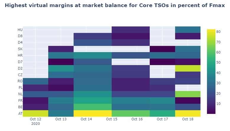
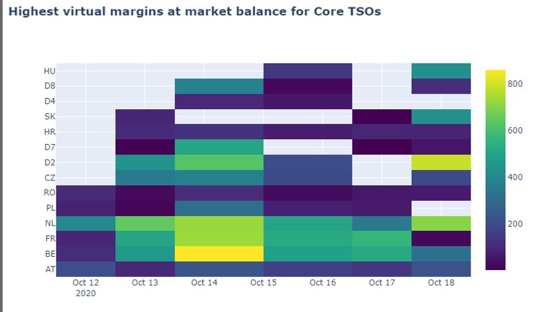
Reading Guide for Capacity Calculation & Market Coupling KPIs

 2.5.2. KPI 14 - Highest virtual margins at MCP per
 TSO, per BD

Short Name of KPI KPI 14a – Highest virtual margins at MCP per TSO
Article in DA CCM -
Granularity Per Business Day
Aggregation Over all CNECs and all timestamps

KPI Description
KPI 14 aims at determining the highest amount of virtual capacity used by the market at the Market Clearing Point (MCP).
The virtual margin (AMR+LTAmargin) represents how much capacity “on top of” Fmax is attributed to the CNE as the result
of initial loadings in the CGM enriched with individual Ramr and LTA inclusion. Before releasing this virtual capacity to
Euphemia, Core TSOs validate during the individual validation step if sufficient remedial actions (RAs) are at disposal to
keep the grid secure should the virtual capacity be used during allocation.
The blank cells in the “heat-table” mean that there was no virtual margin used at MCP on any CNE of one specific TSO on
the concerned BD.
If a graph for a certain set of BDs is not shown then no “virtual margins” were used by the market.
Two flavors of this KPI are visualized: in MW and in relative terms as % of Fmax.
Steps performed to compute the KPI for each CNEC:
 1) Calculate the virtual margin at zero-balance for all CNECs
 'Virtual margin at zero-balance' = -(F_max-FRM-CVA-IVA-F_0core)
 2) Shift to MCP
 'Virtual margin at MCP' = ''Virtual margin at zero-balance + MCPshift
 MCPshift = sum(ptdf*NP) for all Core NP
 3) Filter on positive values to get the additional virtual capacity used by the market

 Version – Date 11-03-2021 Page 18 of 23

Reading Guide for Capacity Calculation & Market Coupling KPIs

Example Visualisation

Short Name of KPI KPI 14b – Highest virtual margins at MCP per TSO
Article in DA CCM -
Granularity Per Business Day
Aggregation Per CNEC and over all timestamps

KPI Description
This KPI is similar to KPI 14a, only here the KPI is depicted for each Core TSO. One dot represents one CNEC.
Example Visualisation

 Version – Date 11-03-2021 Page 19 of 23

Reading Guide for Capacity Calculation & Market Coupling KPIs

 2.5.3. KPI 15 - RAM before and after RAO per TSO

Short Name of KPI KPI 15 - RAM before and after RAO per TSO
Frequency & Audience
KPI Description
 - Will be added once NRAO is added to the CC process.
Example Visualisation

 2.5.4. KPI 16 - Average sensitivity of RAs per TSO

Short Name of KPI KPI 16 - Average sensitivity of RAs per TSO
Frequency & Audience
KPI Description

 Version – Date 11-03-2021 Page 20 of 23

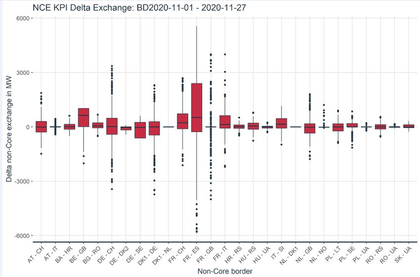
Reading Guide for Capacity Calculation & Market Coupling KPIs

 - Will be added once NRAO is added to the CC process.
Example Visualisation

 2.5.5. KPI 17 - Non-Core exchanges & flow
 deviation on non-Core bidding zone
 borders

Short Name of KPI KPI 17 - Non-Core exchanges & flow deviation on non-Core borders
Article in DA CCM -
Granularity Per bidding zone border
Aggregation Over all CNEs and over reporting period
KPI Description
KPI 17 monitors both the delta exchanges per non-Core border as well as the delta flows per non-Core border, where the delta
refers to the difference between the D-2 and D-1 timeframe forecasts.
Non-Core borders comprise of both EU and non-EU bidding zone borders that are not part of Core but connected to the
bidding zones that also have bidding zone borders in Core (e.g. AT-IT North, DE-DK1, FR-CH or HU-RS).

Delta exchanges on non-Core borders:
 • It illustrates the difference between
 o Best forecast of exchanges on non-Core bidding zone borders (source: D-2 reference program schedule from
 Net Position Forecast used in day-ahead capacity calculation process)
 o Day-ahead scheduled exchanges on the non-Core bidding zone borders (source: ENTSO-E TP)
 • As non-Core exchanges consume capacity on Core CNECs, the delta between the non-Core exchanges in D-2 and
 D-1 is a proxy for the forecast error due to non-Core exchanges on Core CNECs.
 • In case of a DC link or a radial AC border: delta exchange = delta physical flow

Delta flows on non-Core borders:
 • The NPs for all Core bidding zones are shifted from the D-2 NP to the D-1 NP. This delta shift is applied as:

 Δ = Σ s,‰?ŠG × ( ‰•E − ‰•? )

 • which is in line with eq. 6 from Day-Ahead CCM:

 • Consequently, the difference in flow per CNE on non-Core bidding zone borders is derived.
 • Disclaimer: The same PTDFs for D-2 and D-1are used. PTDFs are calculated from the D-2 CGM used in the day-
 ahead capacity calculation process.

Data is processed and aggregated the following way:
 • Computation of either delta exchanges or delta flows is done on a per MTU basis

 Version – Date 11-03-2021 Page 21 of 23

Reading Guide for Capacity Calculation & Market Coupling KPIs

 • CNEs are grouped by bidding zone border
 • Boxplots hold data from grouped CNEs per bidding zone borders and for all considered MTUs

Example Visualisation

 Version – Date 11-03-2021 Page 22 of 23

Reading Guide for Capacity Calculation & Market Coupling KPIs

Version – Date 11-03-2021 Page 23 of 23