Reduction of the chemical master equation for gene regulatory networks using proper generalized decompositions
←
→
Page content transcription
If your browser does not render page correctly, please read the page content below
INTERNATIONAL JOURNAL FOR NUMERICAL METHODS IN BIOMEDICAL ENGINEERING
Int. J. Numer. Meth. Biomed. Engng. 2011; 00:1–15
Published online in Wiley InterScience (www.interscience.wiley.com). DOI: 10.1002/cnm

    Reduction of the chemical master equation for gene regulatory
         networks using proper generalized decompositions

                           Amine Ammar1 , Elı́as Cueto2∗ , Francisco Chinesta3
                                          1 Arts et Metiers ParisTech. Angers, France.
                 2   Aragon Institute of Engineering Research. Universidad de Zaragoza. Zaragoza, Spain.
                      3 EADS Corporate International Chair. Ecole Centrale de Nantes. Nantes, France.

                                                      SUMMARY
The numerical solution of the Chemical Master Equation (CME) governing gene regulatory networks and
cell signaling processes remains a challenging task due to its complexity, exponentially growing with the
number of species involved. While most of the existing techniques rely on the use of Monte Carlo-like
techniques, we present here a new technique based on the approximation of the unknown variable (the
probability of having a particular chemical state) in terms of a finite sum of separable functions. In this
framework, the complexity of the CME grows only linearly with the number of state space dimensions. This
technique generalizes the so-called Hartree approximation, by using as terms as needed in the finite sums
decomposition for ensuring convergence.
But noteworthy, the ease of the approximation allows for an easy treatment of unknown parameters (as is the
case frequently when modeling gene regulatory networks, for instance). These unknown parameters can be
considered as new space dimensions. In this way the proposed method provides solutions for any value of
the unknown parameters (within some interval of arbitrary size) in one execution of the program. Copyright
 c 2011 John Wiley & Sons, Ltd.

Received . . .

KEY WORDS: Gene regulatory networks, chemical master equation, curse of dimensionality, proper
           generalized decomposition

                                                1. INTRODUCTION

When chemically reacting species are present at very low concentrations (in the number of tens
or hundreds of molecules, for instance) the resulting state can not be modeled accurately as
deterministic and the inherent randomness of the system should be taken into account. This is the
case, for instance, when modeling gene regulatory networks. It is well known that small numbers of
molecules can alter these networks significantly [12] [19].
   It is also well known that under some circumstances (a well stirred mixture, fixed volume and
fixed temperature), such a system can be considered Markovian, and that it is governed by the
so-called Chemical Master Equation (CME) [16], which is a set of linear ordinary differential
equations.
   The complexity of the CME comes from the fact that it involves one state space dimension
for each species involved in the reactions. This means that very classic techniques such as finite

∗ Correspondence  to: Aragon Institute of Engineering Research. Universidad de Zaragoza. Edificio Betancourt. Maria de
Luna, s.n., E-50018 Zaragoza, Spain. E-mail: ecueto@unizar.es

Contract/grant sponsor: Spanish Ministry of Innovation and Science; contract/grant number: CICYT-DPI 2011-27778-
C02-01

Copyright c 2011 John Wiley & Sons, Ltd.
Prepared using cnmauth.cls [Version: 2010/03/27 v2.00]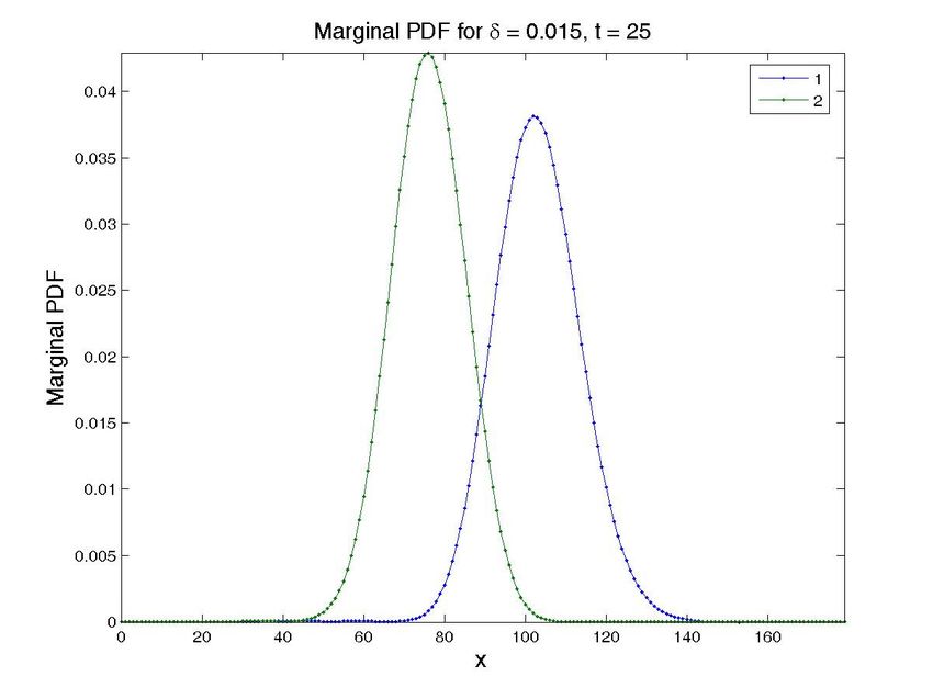
2                                      AMMAR, CUETO, CHINESTA

elements involve a number of degrees of freedom growing exponentially with the number of reacting
species. This difficulty is present in many other branches of Science and Engineering such as the
Schroedinger equation, among others, and has been coined the curse of dimensionality. In practice,
finite element-based techniques are limited by this reason to problems on the order of 20 state space
dimensions [3], by using sparse grid techniques, for instance.
   If we restrict ourselves to the field of cell signalling processes, or in general to the numerical
solution of the CME itself, the so-called Stochastic Simulation Algorithm (SSA) [9] is the most
extended algorithm to this end. Basically, the SSA is a Monte Carlo method, based upon the
realization of individual trajectories within the chemical system. The method can become very
computationally expensive when the system undergoes enormous numbers of individual reactions.
Two different families of alternative methods exist. The first one can be categorized as time-leaping
methods, with the τ -leaping method as the most extended one [10], while the second one separates
slow and fast partitions of the system. For a more detailed analysis see, for instance [16].
   It is well-known, however, that for some simple systems it is necessary to run on the order
of 106 Monte Carlo simulations to achieve the needed precision [16]. On the contrary, models
established for complex systems like, for instance, the cross-talk pathways of IL-1/NF-κB and TGF-
β /Smad involve some 50 different reactions [19], giving a potential state space belonging to N50 (N
represents the set of natural numbers). Considering an interval from 0 to 100 possible copies of
each species, this would give a potential state space comprising on the order of 10100 different
states. Noting that the presumed number of elementary particles in the universe is on the order of
1080 , we clearly take notice of the formidable task of modeling such systems.
   The approach followed herein is completely different. The essential variable of the problem, the
probability of having a particular state on the system, provided an initial state, is approximated
as a finite sum of separable functions. In this way we avoid the burden associated to the curse of
dimensionality and all the variables will be approximated by a sum of tensor products.
   This kind of representation is not new, it was widely employed in the last decades in the
framework of quantum chemistry. In particular the Hartree-Fock (that involves a single product of
functions) and post-Hartree-Fock approaches (as the MCSCF that involves a finite number of sums)
made use of a separated representation of the wave function [4]. In the context of Computational
Mechanics a similar decomposition was proposed, that was called radial approximation, and that
was applied for separating the space and time coordinates in thermomechanical models [14]. In fact,
some prior works that employ Hartree-like approximations for the solution of models established in
the form of a Chemical Master Equation already exist, see [13] and references therein, for instance.
These models assume a particular form of the functions employed along each spatial direction
(usually, Poisson-like distributions, see [18]).
   The approach here presented has been introduced in one of the former works of the authors, see
[1] [2] under the name of Proper Generalized Decompositions (PGD) and then applied in numerous
contexts: (i) quantum chemistry [6]; (ii) Brownian dynamics [5]; (iii) kinetic theory description of
polymers solutions and melts [15]; (iv) kinetic theory descriptions of rod suspensions [17]; among
many others. See [7] [8] for two recent reviews on the topic.
   The outline of the paper is as follows. In the next section we describe the basics of the stochastic
modeling of chemical systems of very low number of molecules. In section 3 we introduce the
essential ingredients of the method, while in section 4 some examples of the performance of the
method are presented.

                             2. THE CHEMICAL MASTER EQUATION

When dealing with chemical system in which the different species are present at very low copy
numbers, it is necessary to work with the number of molecules present at each time instant, instead
of working, as usual, with the concentration of each species. Thus, consider a well mixed system, at
constant volume and temperature, described by the state vector

                                   Z(t) = (#A, #B, #C, #D, . . .)T ,                                  (1)

Copyright c 2011 John Wiley & Sons, Ltd.                        Int. J. Numer. Meth. Biomed. Engng. (2011)
Prepared using cnmauth.cls                                                               DOI: 10.1002/cnm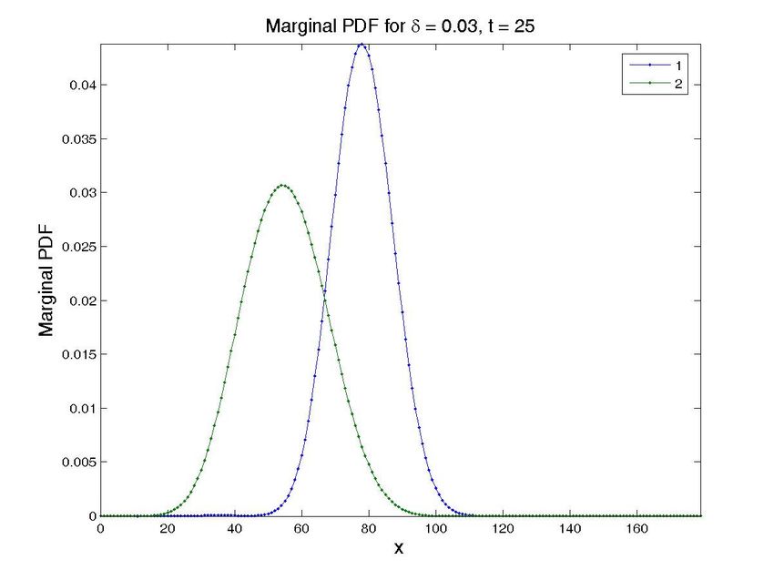
REDUCTION OF THE CME FOR GENE REGULATORY NETWORKS USING PGD                                          3

with initial state Z(t0 ) = z 0 . Here, A, B , etc., represent different chemical species. When some
reaction rj occurs, the system moves from z 0 to z ∗ , where the change in the number of molecules
is equal to its stoichiometry in the reaction rj :

                              rj : sin        in                in
                                    1,j x1 + s2,j x2 + · · · + sN,j xN
                                       kj
                                    GGGGGGAsout       out               out
                                            1,j x1 + s2,j x2 + · · · + sN,j xN ,                                 (2)

with kj the rate constant of reaction rj . In turn, sin,out
                                                     i,j    represent the stoichiometric coefficients of the
i-th species and xk represent the concentrations of each biochemical species.
   This state transition depends on the probability that the changes due to any reaction occur as
described by the propensity function. For any reaction j :

               aj (z)dt ≡ the probability, given Z(t) = z, that rj occurs in [t, t + dt]

  This state transition results in a change of molecules of each species:

                                               v ij = sin     out
                                                       i,j + si,j ,

or, equivalently,
                                                      aj (z − v j )
                                           z − v j GGGGGGGGGGGGGGGAz,                                            (3)

and
                                                   aj (z)
                                              z GGGGGGGGGAz + v j .                                              (4)

  Let us define the probability that each species exists in z number of molecules at any time t:

                        P (z, t|z 0 , t0 ) ≡ Prob{Z(t) = z, given Z(t0 ) = z 0 }.

The CME describes the time evolution of the probability taking into account each propensity aj :
             ∂P (z, t|z 0 , t0 )
                                 =
                   ∂t
                                 X
                                     [aj (z − v j )P (z − v j , t|z 0 , t0 ) − aj (z)P (z, t|z 0 , t0 )] .       (5)
                                j

In compact notation, we will write the CME hereafter as
                                             ∂P (z, t)
                                                       = AP (z, t),                                              (6)
                                                ∂t
where operator A contains the propensities of each reaction:
                                                X
                                           A=       Aj                                                           (7)
                                                           j

  Note that the choice of the probability instead of chemical concentrations as essential variable of
the problem eliminates the need of determining the rate constants of each reaction, and translates
the problem to finding the value of the propensities.

          3. A METHOD BASED ON PROPER GENERALIZED DECOMPOSITIONS

The purposed method is constructed by assuming that the essential variable of the problem, the
probability of having a particular chemical state, is given by a finite sum of separable functions

Copyright c 2011 John Wiley & Sons, Ltd.                                   Int. J. Numer. Meth. Biomed. Engng. (2011)
Prepared using cnmauth.cls                                                                          DOI: 10.1002/cnm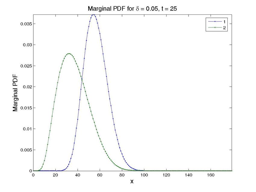
4                                         AMMAR, CUETO, CHINESTA

(separated representation), i.e.,
                                  nF
                                  X
                     P (z, t) =         αj F1j (z1 ) ⊗ F2j (z2 ) ⊗ . . . ⊗ FNj (zN ) ⊗ Ft (t),                 (8)
                                  j=1

where, as mentioned before, the variables zi represent the number of molecules of species i present
at a given time instant. This particular choice of the form of the basis functions allows for an
important reduction in the number of degrees of freedom of the problem, nN × N × nF instead
of (nN )N , where N is the number of dimensions of the state space and nN the number of degrees of
freedom of each one-dimensional grid established for each spatial dimension. For this to be useful,
one has to assume that the probability is negligible outside some interval, and therefore substitute
the infinite domain by a subdomain [0, . . . , m − 1]N , m being the chosen limit number of molecules
for any species in the simulation. A similar assumption is behind other methods in the literature,
such as the Finite State Projection algorithm, for instance [16].
   Another important point to be highlighted is the presence of a function depending solely on time,
Ft (t). This means that the algorithm is not incremental. Instead, it solves for the whole time history
of the chemical species at each iteration of the method.
   The CME is then written in a similar form, as expressed in Eq. (7), by expanding the operator A
in the form
                                       nA
                                       X
                                  A=        Aj1 ⊗ Aj2 ⊗ · · · ⊗ AjN ⊗ I,                            (9)
                                           j=1

where Ai represent the matrix form of each operator Ai involved in the CME and I represents the
identity matrix, acting on the terms depending on time only. Their particular form will be seen
readily.
  An essential ingredient of the method is the way to look for the coefficients αj and also the
particular form of the functions Fij (zi ). This is done in a two-step algorithm consisting of a
projection procedure to determine the coefficients αi and an enrichment procedure to build the
functions Fij (zi ).

3.1. Projection algorithm
Assume that we know a set of suitable functions Fij (zi ). In order to determine the coefficient αj we
put the CME into a weighted form:
                                                ∂P
                                           P∗       = P ∗ AP                                      (10)
                                                ∂t
                           ∗
where the test function P is of the form
                                nF
                                X
                   P ∗ (z, t) =    α∗j F1j (z1 ) ⊗ F2j (z2 ) ⊗ . . . ⊗ FNj (zN ) ⊗ Ft (t).        (11)
                                  j=1

  If we represent Fij by its nodal values collected in vectors F ji , the weighted form of the CME
will have the following matrix expression:
                                  nF X
                                  X  nF                     nF X
                                                            X  nF
                                              ∗i
                                            α Gij α =  j
                                                                      α∗i Hij αj ,                            (12)
                                  i=1 j=1                   i=1 j=1

where                                                                                0
               Gij = (F i1 )T F j1 · (F i2 )T F j2 · . . . · (F iN )T F jN · (F it )T · (F tj )               (13)
        0
with F tj the backward finite difference time derivative of the function F jt and
                  nA
                  X
           Hij =       (F i1 )T Ak1 F j1 · (F i2 )T Ak2 F j2 · . . . ·
                   k=1

                                                                  (F iN )T AkN F jN · (F it )T · (F jt ).     (14)

Copyright c 2011 John Wiley & Sons, Ltd.                                 Int. J. Numer. Meth. Biomed. Engng. (2011)
Prepared using cnmauth.cls                                                                        DOI: 10.1002/cnm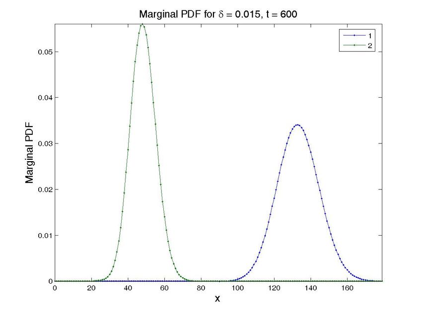
REDUCTION OF THE CME FOR GENE REGULATORY NETWORKS USING PGD 5
Since Eq. (12) must be verified independently of the value of the coefficients α∗i , we arrive
at a nF × nF system of algebraic equations to be solved for the αj . A normality condition of
the probability function is enforced during the solution. To preserve the verification of the initial
condition we assume that α1 = 1 and the first component of Ftj (j ≥ 2) vanishing.
3.2. Enrichment algorithm
If, once solved the system given by Eq. (12) the accuracy of the result is judged not enough, a
method for the enrichment of the basis should be employed. In this case, new functions will be
added to the basis:
nF
X
P (z, t) = α∗j F j1 ⊗ F j2 ⊗ . . . ⊗ F jN ⊗ F t +
j=1
| {z }
PF
R1 ⊗ R2 ⊗ . . . ⊗ RN +1 . (15)
| {z }
PR
In order to determine the functions Ri , we employed a fixed-point alternating directions algorithm,
looking for one Rj at each iteration. Other methods, such as Newton-Raphson algorithm could
equally be employed. In our case, the weighting functions are of the form:
P ∗ = R1 ⊗ R2 ⊗ . . . ⊗ Rj−1 ⊗ R∗j ⊗ Rj+1 ⊗ . . . ⊗ RN +1 , (16)
when we look for the function Rj . In this case, the different terms of the discrete representation are
then given by
XnA N
Y
P ∗ APR = (R∗j )T Akj Rj (Rh )T Akh Rh · (RTN +1 RN +1 ) =
k=1 h=1,h6=j
(R∗j )T Kj Rj (17)
and
nA
X N
Y
P ∗ APF = (R∗j )T Akj F j (Rh )T Akh F h · (RTN +1 F t ) =
k=1 h=1,h6=j
(R∗j )T V j (18)
with their equivalents for the right-hand side
N
∂P R
Y
P∗ = (R∗j )T Rj (Rh )T Rh · (RTN +1 R0N +1 ) =
∂t
h=1,h6=j
(R∗j )T Mj Rj (19)
with R0N +1 the backward finite difference time derivative of the function RN +1 and
N
∂P F
Y
P∗ = (R∗j )T F j (Rh )T F h · (RTN +1 F 0t ) = (R∗j )T W j
(20)
∂t
h=1,h6=j
with F 0t the backward finite difference time derivative of the function F t . This gives rise to a system
of equations of the form
(Mj − Kj )Rj = V j − W j . (21)
For the initial conditions to be verified at subsequent time instants, we take α1 = 1, with the first
value of the new functions F jt (for j ≥ 2) vanishing.
Copyright c 2011 John Wiley & Sons, Ltd. Int. J. Numer. Meth. Biomed. Engng. (2011)
Prepared using cnmauth.cls DOI: 10.1002/cnm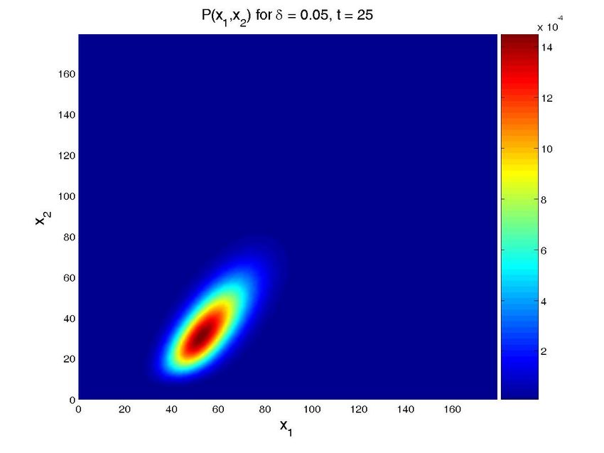
6                                       AMMAR, CUETO, CHINESTA

Figure 1. Schematic mechanism of the toggle switch [12]. The constitutive PL promoter drives the
expression of the lacI gene, which produces the lac repressor tetramer. The lac repressor tetramer binds the
lac operator sites adjacent to the P trc − 2 promoter, thereby blocking transcription of cI . The constitutive
P trc − 2 promoter drives the expression of the cI gene, which produces the λ-repressor dimer. The
λ-repressor dimer cooperatively binds to the operator sites native to the PL promoter, which prevents
                                             transcription of lacI .

Remark 1
The sequence projection-enrichment is iterated until reaching convergence. Two stopping criteria
were considered in our works. The simplest one consists of computing the norm of PR . Despite its
simplicity the convergence is not guaranteed. The other possibility consists of computing the norm
of the equation residual. This stopping criterion ensures the convergence but it is more expensive
from the computational viewpoint.

Remark 2
When convergence is reached, functions Rj are normalized and named FjnF +1 .

Remark 3
We also can use the separated representation introduced before in the framework of an incremental
strategy. This enforces us to solve a problem in dimension N at several time instants. Assuming
known the solution at time t, Pt , the solution at the next time instant can be obtained after solving
the following problem, written as a tensorial product of operators:

                                                  nA
                                                                            !
                                                  X
                         I1 ⊗ . . . ⊗ IN − ∆t ·         Aj1 ⊗ . . . ⊗ AjN       P t+∆t = P t                 (22)
                                                  j=1

In this last equation the right-hand-side term is known and one only needs to find P t+∆t . This
discretization corresponds to an implicit time integration scheme.

                                     4. NUMERICAL EXAMPLES

4.1. Simulation of a toggle switch
The behaviour of the λ-phage virus is one the most studied and well-known examples in gene
regulatory networks. When a bacteriophage λ infects a cell, it either stays dormant or it reproduces
until the cell dies. The resulting behaviour depends crucially on two competing proteins that
inhibit mutually each other, see a schematic representation in Fig. 1. The so-called toggle switch
is composed of a two-gene co-repressive network.

Copyright c 2011 John Wiley & Sons, Ltd.                                Int. J. Numer. Meth. Biomed. Engng. (2011)
Prepared using cnmauth.cls                                                                       DOI: 10.1002/cnm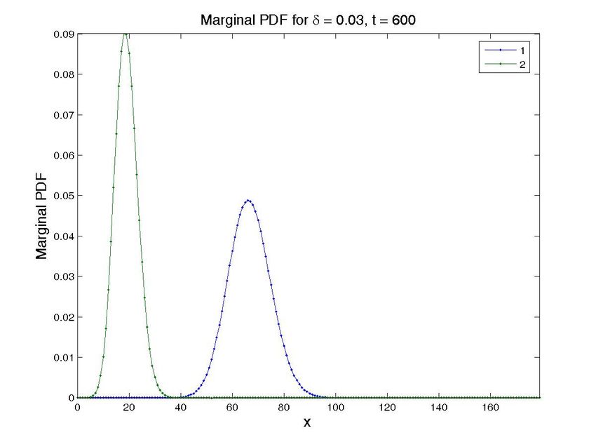
REDUCTION OF THE CME FOR GENE REGULATORY NETWORKS USING PGD                                     7

                                                    Marginal PDF for time = 100

                   0.14
                   0.12                                                  Protein 1
                                                                         Protein 2
                    0.1
    Marginal PDF

                   0.08
                   0.06
                   0.04
                   0.02

                         0               10                20                30                40
                                                                     z

Figure 2. Marginal probability distribution function at t = 100s. Axes denote the number of protein 1 and 2.

                                                    P(z1,z2) for time = 300s                                         −3
                                                                                                               x 10
               0.02
                     0
      −0.02                                                                                                    10
         0

                         20                                                                                    5

                              40
                                                                                              40            50
                               z1                                    20           30                          0
                                    60 0              10
                                                                z2

Figure 3. Solution at steady state (t ≈ 300s) by separation of variables. Axes denote the number of protein
                                     1 (abscissa) and protein 2 (ordinate).

  The operator form of the CME for this example is composed by two terms [11]: A = A1 + A2 ,
given by:

                                                   αβ
                              A1 P (z1 , z2 ) =          P (z1 − 1, z2 ) + δ(z1 + 1) · P (z1 + 1, z2 )−
                                                 β + γz2

                                                  αβ
                                                        + δ · z1 P (z1 , z2 ).                                         (23)
                                                β + γz2

and A2 equivalent with z1 and z2 interchanged. We computed the solution for δ = 0.05, α = 1.0,
γ = 1.0 and β = 0.4.

Copyright c 2011 John Wiley & Sons, Ltd.                                          Int. J. Numer. Meth. Biomed. Engng. (2011)
Prepared using cnmauth.cls                                                                                 DOI: 10.1002/cnm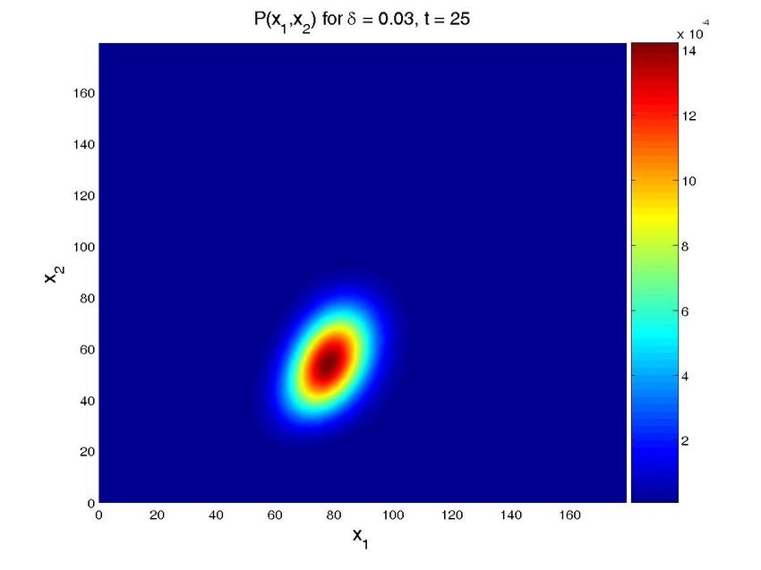
8                                      AMMAR, CUETO, CHINESTA

                              Figure 4. Schematic representation of a cascade.

   The simulation started from a non-physiological state in which both proteins showed a very high
probability around z1 = z2 = 15. Despite this initial state, after t = 100s (Fig. 2) one has a case
where both average values of both proteins and small levels of the one protein combined with higher
level of the other protein are quite likely, and this remains the case for the stationary distribution as
well [11], Fig. 3.

4.2. A cascade of 20 genes
In order to show the potential of the method we have solved a completely academic example,
composed by a cascade of 20 terms. A cascading process occurs when (usually) adjacent genes
produce protein which enhances the expression of the succeeding gene. One typical example can be
found in the lytic phase of the λ-phage system [11], but is composed of substantially fewer terms.
  This example is intended to show the potential of the proposed method, since methods based upon
sparse grids, for instance, rarely can cope with more than 10 proteins [11]. Although completely
academic, we believe that this example clearly demonstrates how a realistic number of different
reactions can be handled without any particular difficulty.
  The operator for this example is composed by twenty terms: A = A1 + . . . + A20 . Operator A1
has the same form as that of the previous example, while the succeeding operators are:

                   βzi−1
    Ai P (z) =             P (z − ei ) + δ(zi + 1)P (z + ei )−
                 βzi−1 + γ

                                                                 βzi−1
                                                                         + δzi P (z), ∀i > 1, (24)
                                                               βzi−1 + γ
where ei is the i-th standard basis of Rn .
   In the cascade the expectations of the marginal distributions have a clear inbuilt delay. As an
example, consider the case of three species with production of the first species α0 = 0.7, decay for
all the species δ = 0.07 and the production of succeeding species equal to zi−1 /(5.0 + zi−1 ) for
i = 2, . . . , 20, respectively, see [11]. The results are depicted in Fig. 5.
   It can be noticed how the size of the bounded domain does not very much influence the resulting
size of the model due to the special separated representation of the variables. Note how, since only
one-dimensional domains are “meshed” for each species, a large domain can be considered without
any special difficulty.
   To compare the proposed method with Hartree-like methods, we conducted the same simulations
but employing only one summand in Eq. (8), i.e., nF = 1. This is, essentially, the main difference
of the proposed method with Hartree approaches. It must be noted, in addition, that no particular
form of the separated function is assumed.
   To see the implication of the use of one summand only, a convergence plot is show in Fig. 6 for
the two cases described before.
   The final result could also be importantly affected. For comparison, we show the final state of the
toggle switch system using only one function and the converged one, as provided by the method,

Copyright c 2011 John Wiley & Sons, Ltd.                           Int. J. Numer. Meth. Biomed. Engng. (2011)
Prepared using cnmauth.cls                                                                  DOI: 10.1002/cnm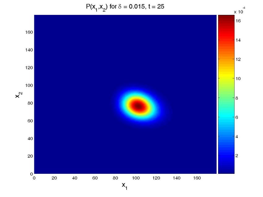
REDUCTION OF THE CME FOR GENE REGULATORY NETWORKS USING PGD 9
Figure 5. The simulation of a cascade composed by 20 terms shows the typical delay that has been observed
for simpler examples.
see Fig. 7. As can be noticed, the result can be quite different and this is particularly noteworthy for
the toggle-switch system.
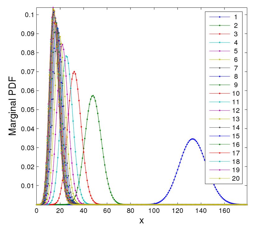
4.3. Simulations in the presence of uncertainty
The most important problem when modeling gene regulatory networks, however, comes from the
fact that many reaction’s parameters are unknowns or very difficult to determine in an easy way
[19]. The easy way in which the method copes with many state space dimensions allows it to handle
unknown parameters in a natural way, by considering them as new state space dimensions, thus
opening the way to designing in silico experiments in which one could eventually observe the effect
of different values of the unknown parameters on the final chemical state of the system.
The transient solution for a particular value of the propensity can then be computed by restricting
the general solution to each particular value of this extra-coordinate. Obviously, the price to be paid
is the increase of the model dimensionality. However, this is not a serious issue when one proceeds
within the separated representation framework just described.
To illustrate this feature, we have simulated a cascade of two terms. The operator related to a
cascade was introduced in the previous section. In order to check the proposed technique, and for
the ease of illustration, we have considered a cascade of only 2 terms, with the parameter δ as an
unknown. Note that the solution (obtained in one execution of the program), see Fig. 8, provides the
solution for different values of δ , that reproduces the ones in the literature [11].
Copyright c 2011 John Wiley & Sons, Ltd. Int. J. Numer. Meth. Biomed. Engng. (2011)
Prepared using cnmauth.cls DOI: 10.1002/cnm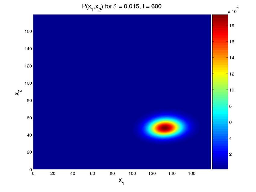
10                                     AMMAR, CUETO, CHINESTA

           −1
        10
                                                                                    switch
                                                                                    cascade

           −2
        10

           −3
        10

           −4
        10

           −5
        10

           −6
        10
                0     2         4          6       8     10       12        14        16       18

Figure 6. Convergence of the result for the toggle-switch and cascade problems (error versus number of
functions employed in the approximation). Note how the use of one-summand approximation could lead to
                                          eventually high errors.

  In order to obtain the solution for a given value of the unknown parameter, one has to cut the
hypercube of the solution by a hyperplane located at a particular value of the variable.

                                               5. CONCLUSIONS

We have presented a technique for the numerical solution of the CME based on the approximation
of the essential variable through a finite sum of separable functions. In this way we can avoid
the burden associated with the curse of dimensionality, i.e., the exponentially-growing number of
degrees of freedom with the number of state space dimensions.
   This strategy allows for a simple method in which time is considered as another variable, such
that all the time history of the system is solved for at each iteration, very much like space-time finite
element techniques. Indeed, unknown parameters of the problem, such as reaction propensities, can
be considered as new state space dimensions. This produces results for any value of the unknown
variable. By cutting the hypercube of the solution field through any hyperplane we readily obtain
the behaviour of the system for particular values of the unknowns.
   This technique avoids the problems related to Monte Carlo-like techniques, such as the burden
associated with high number of dimensions, the need for a large number of realisations of the system
if high accuracy is needed or the lack for appropriate error bounds in the results.
   Of course, it remains to be determined if the method can help to clarify some very complex
systems such as the cross-talk between interleukin-1-induced nuclear factor-κB and TGF-β -induced
Smad pathways, for instance. This system has been modelled by using some 50 different reactions

Copyright c 2011 John Wiley & Sons, Ltd.                          Int. J. Numer. Meth. Biomed. Engng. (2011)
Prepared using cnmauth.cls                                                                 DOI: 10.1002/cnm
REDUCTION OF THE CME FOR GENE REGULATORY NETWORKS USING PGD 11
P(x1,x2) for time = 300 −3
x 10
50
12
45
40 10
35
8
30
2
25
x
6
20
15 4
10
2
5
0
0 10 20 30 40 50
x1
P(x1,x2) for time = 300 −3
x 10
50
14
45
40 12
35 10
30
8
2
25
x
20 6
15
4
10
2
5
0 0
0 10 20 30 40 50
x1
Figure 7. Final state of the toggle-switch model for a Hartree-like model (up) and the converged solution
obtained by the proposed method (down). Axis represent the concentration of each competing protein.
[19], with approximately one half of them not appropriately understood nor characterised. But,
undoubtedly, the presented technique can help to understand the effect of some values of the
unknown variables in the final state of the system.
Copyright c 2011 John Wiley & Sons, Ltd. Int. J. Numer. Meth. Biomed. Engng. (2011)
Prepared using cnmauth.cls DOI: 10.1002/cnm12 AMMAR, CUETO, CHINESTA
Figure 8. Solution for the cascade problem with unknown propensities. Probability distribution function (top
row) and marginal probability distribution function of each species (bottom row) at time t = 0, t = 30s, and
t = 600s (approx. steady state). The left column present the results for a value δ = 0.015, while the central
one is for δ = 0.03 and the left one for δ = 0.05. Note that all the results are obtained in one execution
of the program. The four-dimensional hypercube containing the solution space, whose dimensions are the
concentrations of the two proteins, the value of δ and time, is then cut by the hyperplanes defined by the
different values of δ and time to give these plots.
Copyright c 2011 John Wiley & Sons, Ltd. Int. J. Numer. Meth. Biomed. Engng. (2011)
Prepared using cnmauth.cls DOI: 10.1002/cnmREDUCTION OF THE CME FOR GENE REGULATORY NETWORKS USING PGD 13
ACKNOWLEDGEMENTS
This work has been partially funded by the Spanish Ministry of Science and Innovation, through
grant number CICTY-DPI2011-27778-C02-01, whose help is gratefully acknowledged.
A. DISCRETE FORMS
In order to make a discrete form of the equations of the cascade model we need to define some
matrices. These matrices are related to each species ‘i’ and their associated size is equal to
(mi × mi ), the number of operators in the model. The identity matrices will be denoted
1 0 ··· 0
.. ..
0 1 . .
Ii = ..
(25)
.. ..
. . . 0
0 ··· 0 1
Two other matrices are also required to define the shift allowing to get the neighbouring probability
0 1 0 ··· 0
.. ..
0 0 1 . .
+
Ii = .. .. .. .. (26)
. . . . 0
1
0 ··· 0 0
0 0 ··· 0
.. ..
1 0 . .
−
Ii =
..
(27)
0 1 .
.. .. ..
. . . 0
0 ··· 0 1 0
According to these definitions one can write each operator Ai in terms of tensorial product of
operators applied on each dimension that consists of {0, . . . , mi−1 } components. The first operator
writes
1 ··· 00
. . ..
−
0 2 . . +
A1 =
α · I1 + δ ·
.. . . . .
· I − α · I1 −
1
. . . 0
0 ··· 0 m1
0 0 ··· 0
. . ..
0 1 . .
δ· .
⊗ I2 ⊗ ... ⊗ IN (28)
.. . .
.. .. 0
0 ··· 0 m1 − 1
Copyright c 2011 John Wiley & Sons, Ltd. Int. J. Numer. Meth. Biomed. Engng. (2011)
Prepared using cnmauth.cls DOI: 10.1002/cnm14 AMMAR, CUETO, CHINESTA
that defines a single tensor product. For i > 1 the operator Ai consists of 4 tensor products:
a(0) 0 ··· 0
. .
a(1) . . ..
0
⊗ I− ⊗ Ii+1 ⊗ . . . ⊗ IN +
Ai = I1 ⊗ . . . ⊗ Ii−2 ⊗ .
i
.. . .. . .. 0
0 ··· 0 a(mi−1 − 1)
1 0 ··· 0
. . ..
0 2 . . · I+ ⊗ Ii+1 ⊗ . . . ⊗ IN −
δ · I1 ⊗ . . . ⊗ Ii−1 ⊗ .
i
.. . .
.. .. 0
0 ··· 0 mi
a(0) 0 ··· 0
. .
a(1) . . ..
0
− I1 ⊗ . . . ⊗ Ii−2 ⊗ ..
⊗ Ii ⊗ Ii+1 ⊗ . . . ⊗ IN −
.. ..
. . . 0
0 ··· 0 a(mi−1 − 1)
0 0 ··· 0
. . ..
0 1 . .
− δ · I1 ⊗ . . . ⊗ Ii−1 ⊗ .
· Ii ⊗ Ii+1 ⊗ . . . ⊗ IN (29)
.. . .
.. .. 0
0 ··· 0 mi − 1
where
βy
a(y) = . (30)
βy + γ
REFERENCES
1. A. Ammar, B. Mokdad, F. Chinesta, and R. Keunings. A new family of solvers for some classes of multidimensional
partial differential equations encountered in kinetic theory modeling of complex fluids. J. Non-Newtonian Fluid
Mech., 139:153–176, 2006.
2. A. Ammar, B. Mokdad, F. Chinesta, and R. Keunings. A new family of solvers for some classes of multidimensional
partial differential equations encountered in kinetic theory modeling of complex fluids. part ii: transient simulation
using space-time separated representations. J. Non-Newtonian Fluid Mech., 144:98–121, 2007.
3. H.-J. Bungartz and M. Griebel. Sparse grids. Acta Numerica, 13:1–123, 2004.
4. E. Cancès, M. Defranceschi, W. Kutzelnigg, C. Le Bris, and Y. Maday. Computational quantum chemistry: a
primer. In Handbook of Numerical Analysis, volume X, pages 3–270, 2003.
5. F. Chinesta, A. Ammar, A. Falco, and M. Laso. On the reduction of stochastic kinetic theory models of complex
fluids. Modeling and Simulation in Materials Science and Engineering, 15:639–652, 2007.
6. F. Chinesta, A. Ammar, and P. Joyot. The nanometric and micrometric scales of the structure and mechanics of
materials revisited: An introduction to the challenges of fully deterministic numerical descriptions. International
Journal for Multiscale Computational Engineering, 6:191–213, 2008.
7. Francisco Chinesta, Amine Ammar, and Elias Cueto. Recent advances and new challenges in the use of the
proper generalized decomposition for solving multidimensional models. Archives of Computational Methods in
Engineering, 17:327–350, 2010.
8. Francisco Chinesta, Pierre Ladeveze, and Elias Cueto. A short review on model order reduction based on proper
generalized decomposition. Archives of Computational Methods in Engineering, 18:395–404, 2011.
9. D. T. Gillespie. Exact stochastic simulation of coupled chemical reactions. The Journal of Physical Chemistry,
81(25):2340–2361, 1977.
10. D. T. Gillespie. Approximate accelerated stochastic simulation of chemically reacting systems. The Journal of
Chemical Physics, 115:1716–1733, 2001.
11. M. Hegland, C. Burden, L. Santoso, S. MacNamara, and H. Boothm. A solver for the stochastic master equation
applied to gene regulatory networks. Journal of Computational and Applied Mathematics, 205:708–724, 2007.
12. J.Hasty, D. McMillen, F. Isaacs, and J. J. Collins. Computational studies of gene regulatory networks: in numero
molecular Biology. Nature Reviews Genetics, 2:268–279, 2001.
13. K.-Y. Kim and J. Wang. Potential energy landscape and robustness of a gene regulatory network: toggle switch.
PLoS Computational Biology, 3:0565–0577, 2007.
14. P. Ladeveze. Nonlinear Computational Structural Mechanics. Springer, N.Y., 1999.
Copyright c 2011 John Wiley & Sons, Ltd. Int. J. Numer. Meth. Biomed. Engng. (2011)
Prepared using cnmauth.cls DOI: 10.1002/cnmREDUCTION OF THE CME FOR GENE REGULATORY NETWORKS USING PGD 15
15. B. Mokdad, E. Pruliere, A. Ammar, and F. Chinesta. On the simulation of kinetic theory models of complex fluids
using the fokker-planck approach. Applied Rheology, 17:1–14, 2007.
16. B. Munsky and M. Khammash. The finite state projection algorithm for the solution of the chemical master
equation. The Journal of Chemical Physics, 124(4):044104, 2006.
17. E. Pruliere, A. Ammar, N. El Kissi, and F. Chinesta. Multiscale modelling of flows involving short fiber
suspensions. Archives of Computational Methods in Engineering, 16:1–30, 2009.
18. M. Sasai and P. G. Wolynes. Stochastic gene expression as a many-body problem. Proceedings of the National
Academy of Sciences, 100(5):2374–2379, 2003.
19. S. N. Sreenath, K-H Cho, and P. Wellstead. Modelling the dynamics of signalling pathways. Essays in
biochemistry, 45:1–28, 2008.
Copyright c 2011 John Wiley & Sons, Ltd. Int. J. Numer. Meth. Biomed. Engng. (2011)
Prepared using cnmauth.cls DOI: 10.1002/cnmYou can also read