REINFORCEMENT LEARNING WITH LATENT FLOW
←
→
Page content transcription
If your browser does not render page correctly, please read the page content below
R EINFORCEMENT L EARNING WITH L ATENT F LOW
                                         Wenling Shang2,† , Xiaofei Wang1,† ,
                                         Aravind Srinivas1 , Aravind Rajeswaran3 , Yang Gao1 ,
                                         Pieter Abbeel1 & Michael Laskin1
                                         University of California Berkeley1 , Deepmind2 , University of Washington3

                                                                                     A BSTRACT
arXiv:2101.01857v1 [cs.LG] 6 Jan 2021

                                                 Temporal information is essential to learning effective policies with Reinforcement
                                                 Learning (RL). However, current state-of-the-art RL algorithms either assume
                                                 that such information is given as part of the state space or, when learning from
                                                 pixels, use the simple heuristic of frame-stacking to implicitly capture temporal
                                                 information present in the image observations. This heuristic is in contrast to
                                                 the current paradigm in video classification architectures, which utilize explicit
                                                 encodings of temporal information through methods such as optical flow and
                                                 two-stream architectures to achieve state-of-the-art performance. Inspired by
                                                 leading video classification architectures, we introduce the Flow of Latents for
                                                 Reinforcement Learning (Flare), a network architecture for RL that explicitly
                                                 encodes temporal information through latent vector differences. We show that
                                                 Flare (i) recovers optimal performance in state-based RL without explicit access
                                                 to the state velocity, solely with positional state information, (ii) achieves state-of-
                                                 the-art performance on pixel-based challenging continuous control tasks within
                                                 the DeepMind control benchmark suite, namely quadruped walk, hopper hop,
                                                 finger turn hard, pendulum swing, and walker run, and is the most sample efficient
                                                 model-free pixel-based RL algorithm, outperforming the prior model-free state-of-
                                                 the-art by 1.9× and 1.5× on the 500k and 1M step benchmarks, respectively, and
                                                 (iv), when augmented over rainbow DQN, outperforms this state-of-the-art level
                                                 baseline on 5 of 8 challenging Atari games at 100M time step benchmark.

                                        1    I NTRODUCTION

                                        Reinforcement learning (RL) (Sutton & Barto, 1998) holds the promise of enabling artificial agents to
                                        solve a diverse set of tasks in uncertain and unstructured environments. Recent developments in RL
                                        with deep neural networks have led to tremendous advances in autonomous decision making. Notable
                                        examples include classical board games (Silver et al., 2016; 2017), video games (Mnih et al., 2015;
                                        Berner et al., 2019; Vinyals et al., 2019), and continuous control (Schulman et al., 2017; Lillicrap
                                        et al., 2016; Rajeswaran et al., 2018). A large body of research has focused on the case where an
                                        RL agent is equipped with a compact state representation. Such compact state representations are
                                        typically available in simulation (Todorov et al., 2012; Tassa et al., 2018) or in laboratories equipped
                                        with elaborate motion capture systems (OpenAI et al., 2018; Zhu et al., 2019; Lowrey et al., 2018).
                                        However, state representations are seldom available in unstructured real-world settings like the home.
                                        For RL agents to be truly autonomous and widely applicable, sample efficiency and the ability to act
                                        using raw sensory observations like pixels is crucial. Motivated by this understanding, we study the
                                        problem of efficient and effective deep RL from pixels.
                                        A number of recent works have made progress towards closing the sample-efficiency and performance
                                        gap between deep RL from states and pixels (Laskin et al., 2020b;a; Hafner et al., 2019a; Kostrikov
                                        et al., 2020). An important component in this endeavor has been the extraction of high quality
                                        visual features during the RL process. Laskin et al. (2020a) and Stooke et al. (2020) have shown
                                        that features learned either explicitly with auxiliary losses (reconstruction or contrastive losses)
                                        or implicitly (through data augmentation) are sufficiently informative to recover the agent’s pose
                                           †: equal contribution. Correspondence: wendyshang@google.com. Code: https://github.com/
                                        WendyShang/flare.

                                                                                            1
information. While existing methods can encode positional information from images, there has
been little attention devoted to extracting temporal information from a stream of images. As a
result, existing deep RL methods from pixels struggle to learn effective policies on more challenging
continuous control environments that deal with partial observability, sparse rewards, or those that
require precise manipulation.
Current approaches in deep RL for learning tem-
poral features are largely heuristic in nature. A                   t
commonly employed approach is to stack the
most recent frames (Mnih et al., 2015) as in-                                                  _
puts to a convolutional neural network (CNN).
                                                                   t-1
This can be interpreted as a form of early fu-                                                   RL
sion (Karpathy et al., 2014), where information                                                _
from the recent time window is combined imme-
diately at the pixel level for input to the CNN.                   t-2

In contrast, modern video recognition systems
use alternate architectures that employ optical
flow and late fusion (Simonyan & Zisserman,                 Latent        Latent   _ Subtraction
2014), where frames are processed individually              Vectors    Differences
with CNN layers before fusion and downstream
processing. Such a late fusion approach is typi- Figure 1: Flow of Latents for Reinforcement
cally beneficial due to better performance, fewer Learning (Flare) architecture. Input frames are
parameters, and the ability to use multi-modal first encoded individually by the same encoder.
data (Chebotar et al., 2017; Jain et al., 2019). The resulting latent vectors are then concatenated
However, directly extending such architectures with their latent differences before being passed to
to RL is be challenging. Real-time computation the downstream RL algorithm.
of optical flow for action selection can be computationally infeasible for many applications with
fast control loops like robotics. Furthermore, optical flow computation at training time can also be
prohibitively expensive. In our experiments, we also find that a naive late fusion architecture minus
the optical flow yields poor results in RL settings (see Section 5.2). This observation is consistent
with recent findings in related domains like visual navigation (Walsman et al., 2019).
To overcome the above challenges, we develop Flow of Latents for Reinforcement Learning (Flare),
a new architecture for deep RL from pixels (Figure 1). Flare can be interpreted as a structured late
fusion architecture. Flare processes each frame individually to compute latent vectors, similar to
a standard late fusion approach (see Figure 1). Subsequently, temporal differences between the
latent feature vectors are computed and fused along with the latent vectors by concatenation for
downstream processing. By incorporating this structure of temporal difference in latent feature space,
we provide the learning agent with appropriate inductive bias. In experiments, we show that Flare (i)
recovers optimal performance in state-based RL without explicit access to the state velocity, solely
with positional state information, (ii) achieves state-of-the-art performance compared to model-free
methods on several challenging pixel-based continuous control tasks within the DeepMind control
benchmark suite, namely Quadruped Walk, Hopper Hop, Finger Turn-hard, Pendulum Swingup,
and Walker Run, while being the most sample efficient model-free pixel-based RL algorithm across
these tasks, outperforming the prior model-free state-of-the-art RAD by 1.9× and 1.5× on the 500k
and 1M environment step benchmarks, respectively, and (iii) when augmented over Rainbow DQN,
outperforms the baseline on 5 out of 8 challenging Atari games at 100M step benchmark.

2   R ELATED W ORK

Pixel-Based RL The ability of an agent to autonomously learn control policies from visual inputs
can greatly expand the applicability of deep RL (Dosovitskiy et al., 2017; Savva et al., 2019). Prior
works have used CNNs to extend RL algorithms like PPO (Schulman et al., 2017), SAC (Haarnoja
et al., 2018), and Rainbow (Hessel et al., 2017) to pixel-based tasks. Such direct extensions have
typically required substantially larger number of environment interactions when compared to the
state-based environments. In order to improve sample efficiency, recent efforts have studied the
use of auxiliary tasks and loss functions (Yarats et al., 2019; Laskin et al., 2020b; Schwarzer et al.,
2020), data augmentation (Laskin et al., 2020a; Kostrikov et al., 2020), and latent space dynamics
modeling (Hafner et al., 2019b;a). Despite these advances, there is still a large gap between the

                                                  2
learning efficiency in state-based and pixel-based environments in a number of challenging benchmark
tasks. Our goal in this work is to identify where and how to improve pixel-based performance on this
set of challenging control environments.
Neural Network Architectures in RL The work of Mnih et al. (2015) combined Q-learning with
CNNs to achieve human level performance in Atari games, wherein Mnih et al. (2015) concatenate the
most recent 4 frames and use a convolutional neural network to output the Q values. In 2016, Mnih
et al. (2016) proposed to use a shared CNN among frames to extract visual features and aggregate
the temporal information with LSTM. The same architectures have been adopted by most works to
date (Laskin et al., 2020b; Schwarzer et al., 2020; Kostrikov et al., 2020; Laskin et al., 2020a). The
development of new architectures to better capture temporal information in a stream of images has
received little attention in deep RL, and our work fills this void. Perhaps the closest to our motivation
is the work of Amiranashvili et al. (2018) who explicitly use optical flow as an extra input to the RL
policy. However, this approach requires additional information and supervision signal to train the
flow estimator, which could be unavailable or inaccurate in practice. In contrast, our approach is a
simple modification to existing deep RL architectures and does not require any additional auxiliary
tasks or supervision signals.
Two-Stream Video Classification In video classification tasks, such as activity recognition (Soomro
et al., 2012), there are a large body of works on how to utilize temporal information (Donahue et al.,
2015; Ji et al., 2012; Tran et al., 2015; Carreira & Zisserman, 2017; Wang et al., 2018; Feichtenhofer
et al., 2019). Of particular relevance is the two-stream architecture of Simonyan & Zisserman (2014),
where one CNN stream takes the usual RGB frames, while the other the optical flow computed from
the RGB values. The features from both streams are then late-fused to predict the activity class. That
the two-stream architecture yields a significant performance gain compared to the single RGB stream
counterpart, indicating the explicit temporal information carried by the flow plays an essential role in
video understanding. Instead of directly computing the optical flow, we propose to capture the motion
information in latent space to avoid computational overheads and potential flow approximation errors.
Our approach also could focus on domain-specific motions that might be overlooked in a generic
optical flow representation.
3 M OTIVATION
Environment Step
Full-state SAC Flare Position-only SAC
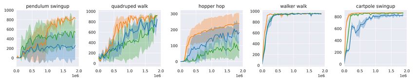
Figure 2: Flare enables an RL agent with only access to positional state to recover a near-optimal
policy relative to RL with access to the full state. In the above learning curves we show test-time
performance for (i) full-state SAC (blue), where both pose and temporal information is given (ii)
position-only SAC (green), and (iii) state-based Flare (orange), where only pose information is
provided and velocities are approximated through pose offsets. Unlike full-state SAC, which learns
the optimal policy, position-only SAC either fails or converges at suboptimal policies. Meanwhile,
the fusion of positions and approximated velocities in Flare efficiently recovers near-optimal policies
in most cases. This motivates using Flare for pixel-based input, where velocities are not present in the
observation. These results show mean performance with standard deviations averaged over 3 seeds.
We motivate Flare by investigating the importance of temporal information in state-based RL.
Our investigation utilizes 5 diverse DMControl (Tassa et al., 2018) tasks. The full state for these
environments includes both the agent’s pose information, such as the joints’ positions and angles, as
well as temporal information, such as the joints’ translational and angular velocities. We train two
variants with SAC—one where the agent receives the full state as input (full-state SAC), and the other
with the temporal information masked out, i.e. the agent only receives the pose information as its
input (position-only SAC). The resulting learning curves are in Figure 2. While the full-state SAC
learns the optimal policy quickly, the position-only SAC learns much sub-optimal policies, which
3
often fail entirely. Therefore, we conclude that effective policies cannot be learned from positions
alone, and that temporal information is crucial for efficient learning.
While full-state SAC can receive velocity information from internal sensors in simulation, in the more
general case such as learning from pixels, such information is often not readily available. For this rea-
son, we attempt to approximate temporal information as the difference between two consecutive states’
positions. Concretely, we compute the positional offset δt =(spt −spt−1 , spt−1 −spt−2 , spt−2 −spt−3 ), and
provide the fused vector (spt , δt ) to the SAC agent. This procedure describes the state-based version
of Flare. Results shown in Figure 2 demonstrate that state-based Flare significantly outperforms
the position-only SAC. Furthermore, it achieves optimal asymptotic performance and a learning
efficiency comparable to full-state SAC in most environments.

                                                       Environment Step
                                                                                      Flare      Recurrent     Stack SAC

Figure 3: We compare 3 ways to incorporate temporal information: i) Flare (orange) receives
(spt , spt −spt−1 , spt−1 −spt−2 , spt−2 −spt−3 ), ii) stack SAC (green) stacks (spt , spt−1 , spt−2 , spt−3 ) as inputs,
and iii) recurrent SAC (blue) uses recurrent layers to process (spt , spt−1 , spt−2 , spt−3 ). Stack SAC and
recurrent SAC perform significantly worse than Flare on most environments, highlighting the benefit
of how Flare handles temporal information. Results are averaged over 3 seeds.
Given that the position-only SAC utilizes spt compared to Flare that utilizes spt and δt , we also investi-
gate a variant (stack SAC) where the SAC agent takes consecutive positions (spt , spt−1 , spt−2 , spt−3 ).
Stack SAC reflects the frame-stack heuristic used in pixel-based RL. Results in Figure 3 show that
Flare still significantly outperforms stack SAC. It suggests that the well-structured inductive bias in
the form of temporal-position fusion is essential for efficient learning.
Lastly, since a recurrent structure is an alternative approach to process temporal information, we im-
plement an SAC variant with recurrent modules (Recurrent SAC) to compare with Flare. Specifically,
we pass a sequence of poses spt , spt−1 , spt−2 , spt−3 through an LSTM cell. The number of the LSTM
hidden units h is set to be the same as the dimension of δt in Flare. The trainable parameters of the
LSTM cell are updated to minimize the critic loss. Recurrent SAC is more complex to implement
and requires longer wall-clock training time, but performs worse than Flare as shown in Figure 3.
Our findings from the state experiments in Figure 2 and Figure 3 suggest that (i) temporal information
is crucial to learning effective policies in RL, (ii) using Flare to approximate temporal information
in the absence of sensors that provide explicit measurements is sufficient in most cases, and (iii) to
incorporate temporal information via naively staking position states or a recurrent module are less
effective than Flare. In the next section, we carry over these insights to pixel-space RL.

4     R EINFORCEMENT L EARNING WITH L ATENT F LOW
To date, frame stacking is the most common way of pre-processing pixel-based input to convey
temporal information for RL algorithms. This heuristic, introduced by Mnih et al. (2015), has been
largely untouched since its inception and is used in most state-of-the-art RL architectures. However,
our observations from the experiments run on state inputs in Section 3 suggest an alternative to the
frame stacking heuristic through the explicit inclusion of temporal information as part of the input.
Following this insight, we seek a general alternative approach to explicitly incorporate temporal
information that can be coupled to any base RL algorithm with minimal modification. To this end,
we propose the Flow of Latents for Reinforcement Learning (Flare) architecture. Our proposed
method calculates differences between the latent encodings of individual frames and fuses the feature
differences and latent embeddings before passing them as input to the base RL algorithm, as shown
in Figure 4. We demonstrate Flare on top of 2 state-of-the-art model-free off-policy RL baselines,
RAD-SAC (Laskin et al., 2020a) and Rainbow DQN (Hessel et al., 2017), though in principle any RL
algorithm can be used in principle.

                                                             4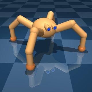
Fusion by
                                                                        Concatenation

                                               ot                                                 ot               zt
                                                                                                                   δt
                                   πψ                                      πψ                                                    πψ
                                               ot−1                                               ot−1             zt−1

                                   Qϕ                                      Qϕ                                      δt−1         Qϕ
(ot, ot−1, ot−2)                               ot−2                                               ot−2             zt−2

                                                                                                                δt−k = zt−k − zt−2k

    (a) Frame stacking heuristic        (b) Individual frame encoding                   (c) Flow of Latents for RL (Flare)

Figure 4: Flow of Latents for Reinforcement Learning (Flare): (a) the architecture for the frame
stacking heuristic, (b) an alternative to the frame stacking hueristic by encoding each image indi-
vidually, and (c) the Flare architecture which encodes images individually, computes the feature
differences, and fuses the differences together with the latents.

4.1        L ATENT F LOW

In computer vision, the most common way to explicitly inject temporal information of a video
sequence is to compute dense optical flow between consecutive frames (Simonyan & Zisserman,
2014). Then the RGB and the optical flow inputs are individually fed into two streams of encoders
and the features from both are fused in the later stage of the piple. But two-stream architectures with
optical flow are not as applicable to RL, because it is too computationally costly to generate optical
flow on the fly.
To address this challenge and motivated by experiments in Section 3, we propose an alternative
architecture that is similar in spirit to the two-stream networks for video classification. Rather than
computing optical flow directly, we approximate temporal information in the latent space. Instead of
encoding a stack of frames at once, we use a frame-wise CNN to encode each individual frame. Then
we compute the differences between the latent encodings of consecutive frames, which we refer to as
latent flow. Finally, the latent features and the latent flow are fused together through concatenation
before getting passed to the downstream RL algorithm. We call the proposed architecture as Flow of
Latents for Reinforcement Learning (Flare).

4.2        I MPLEMENTATION D ETAILS

                                                                 For clarity of exposition, we select RAD as
                                                                 the base algorithm to elaborate the execution
Algorithm 1: Pixel-based Flare Inference                         of Flare. Also, we use RAD later on in our
Given πψ , fCNN ;                                                experiments as the comparative baseline (Sec-
for each environment step t do                                   tion 5). The RAD architecture, shown in Fig-
    zj =fCNN (oj ), j=t−k, .., t;                                ure 4a, stacks multiple data augmented frames
    δj =zj −zj−1 , j=t−k+1, .., t;                               observed in the pixel space and encodes them
    zt =(zt−k+1 , · · ·, zt , δt−k+1 , · · ·, δt );              altogether through an CNN. This can be viewed
    zt = LayerNorm(fFC (zt ));                                   as a form of early fusion (Karpathy et al., 2014).
    at ∼πψ (at |zt );
    ot+1 ∼p(ot+1 |at , ot = (ot , ot−1 ..ot−k ));      Another preprocessing option is to encode each
                                                       frame individually through a shared frame-wise
end
                                                       encoder and perform late fusion of the resulting
                                                       latent features, as shown in Figure 4b. However,
we find that simply concatenating the latent features results in inferior performance when compared to
the frame stacking heuristic, which we further elaborate in Section 5.2. We conjecture that pixel-level
frame stacking benefits from leveraging both the CNN and the fully connected layers to process
temporal information, whereas latent-level stacking does not propagate temporal information back
through the CNN encoder.

                                                            5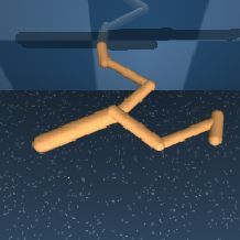
Task              Flare (500K)     RAD (500K)        Flare (1M)   RAD (1M)
           Quadruped Walk           296 ± 139        206 ± 112        488 ± 221    322 ± 229
          Pendulum Swingup          242 ± 152         79 ± 73         809 ± 31     520 ± 321
             Hopper Hop              90 ± 55           40 ± 41        217 ± 59      211 ± 27
           Finger Turn hard         282 ± 67          137 ± 98        661 ± 315     249 ± 98
             Walker Run              426 ± 33        547 ± 48          556 ± 93    628 ± 39
Table 1: Evaluation on 5 benchmark tasks around 500K and 1M environment steps. We evaluate over 5 seeds,
each of 10 trajectories and show the mean ± standard deviation across runs.
                    Rainbow             Flare                              Rainbow           Flare
  Assault         15229±3603         12724±1107           Breakout         280±18           345±22
  Berserk          1636±598           2049±421            Defender       44694±3984      86982±29214
 Montezuma          900±807          1668±1055            Seaquest      24090±12474       13901±8085
  Phoenix         16992±3295        60974±18044          Tutankham         247±11           248±20
           Table 2: Evaluation on 8 benchmark Atari games at 100M training steps over 5 seeds.
Based on this conjecture, we explicitly compute the latent flow δt = zt − zt−1 while detaching the
zt−1 gradients when computing δt . We then fuse together (δt , zt ). Next, since negative values in the
fused latent embedding now possesses semantic meaning from δt , instead of ReLU non-linearity, we
pass the embedding through a fully-connected layer followed by layer normalization, before entering
the actor and critic networks as shown in Figure 4c. Pseudocode illustrates inference with Flare in
Algorithm 1; during training, the encodings of latent features and flow are done in the same way
except with augmented observations.

5     E XPERIMENTS
In this section, we first present the main experimental results, where we show that Flare achieves
substantial performance gains over the base algorithm RAD (Laskin et al., 2020a). Then we conduct
a series of ablation studies to stress test the design choices of the Flare architecture. In the appendix,
we introduce the 5 continuous control tasks from DMControl suite (Tassa et al., 2018) and 8 Atari
games (Bellemare et al., 2013) that our experiments focus on in the Appendix.

5.1   M AIN R ESULTS

DMControl: Our main experimental results on the 5 DMControl tasks are presented in Figure 5 and
Table 1. We find that Flare outperforms RAD in terms of both final performance and sample efficiency
for majority (3 out of 5) of the environments, while being competitive on the remaining environments.
Specifically, Flare attains similar asymptotic performance to state-based RL on Pendulum Swingup,
Hopper Hop, and Finger Turn-hard. For Quadruped Walk, a particularly challenging environment
due to its large action space and partial observability, Flare learns much more efficiently than RAD
and achieves a higher final score. Moreover, Flare outperforms RAD in terms of sample efficiency on
all of the core tasks except for Walker Run as shown in Figure 5. The 500k and 1M environment step
evaluations in Table 1 show that, on average, Flare achieves 1.9× and 1.5× higher scores than RAD
at the 500k step and the 1M step benchmarks, respectively.
Atari: The results on the 8 Atari games are in Figure 6 and Table 3. Here the baseline Rainbow
DQN’s model architecture is modified to match that of Flare, including increasing the number of last
layer convolutional channels and adding a fully-connected layer plus layer normalization before the
Q networks. Again, we observe substantial performance gain from Flare on the majority (5 out of 8)
of the games, including the challenging Montezuma’s Revenge. On most of the remaining games,
Flare is equally competitive except for Seaquest. In Appendix A.3, we also show that Flare performs
competitively when comparing against other DQN variants at 100M training steps, including the
original Rainbow implementations.

5.2   A BLATION S TUDIES

We ablate a number of components of the Flare architecture on the Quadruped Walk and Pendulum
Swingup environments to stress test the Flare architecture. The results shown in Figure 7 aim to
answer the following questions:

                                                     6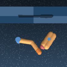
Episode Return

                                                 Environment Step
                                                                             RAD      Flare      State-SAC

Figure 5: We compare Flare and the current STOA model-free baseline RAD on 5 challenging
DMControl environments. Pendulum Swingup are trained over 1.5e6 and the rest 2.5e6. Flare
substantially outperforms RAD on a majority (3 out of the 5) of environments, while being competitive
in the remaining. Results are averaged over 5 random seeds with standard deviation (shaded regions).

                                                                                   Rainbow DQN       Flare

Figure 6: We compare Rainbow DQN and Flare on 8 Atari games over 100M training steps. Flare
substantially enhances 5 out of 8 games over the baseline Rainbow DQN while matching the rest
except Seaquest. Results are averaged over 5 random seeds with standard deviation (shaded regions).

Q1: Do we need latent flow or is computing pixel differences sufficient?
A1: Flare proposes a late fusion of latent differences with the latent embeddings, while a simpler
approach is an early fusion of pixel differences with the pixel input, which we call pixel flow. We
compare Flare to pixel flow in Figure 7 (left) and find that pixel flow is above RAD but significantly
less efficient and less stable than Flare, particularly on Quadruped Walk. This ablation suggests that
late fusion temporal information after encoding the image is preferred to early fusion.
Q2: Are the gains coming from latent flow or individual frame-wise encoding?
A2: Next, we address the potential concern that the performance gain of Flare stems from the frame-
wise ConvNet architectural modification instead of the fusion of latent flow. Concretely, we follow the
exact architecture and training as Flare, but instead of concatenating the latent flow, we concatenate
each frame’s latent vector after the convolution encoders directly as described in Figure 4b. This
ablation is similar in spirit to the state-based experiments in Figure 3. The learning curves in Figure 7
(center) show that individual frame-wise encoding is not the source of the performance lift: frame-
wise encoding, though on par with RAD on Pendulum Swingup, performs significantly worse on
Quadruped Walk. Flare’s improvements over RAD are therefore most likely a result of the explicit
fusion of latent flow.
Q3: How does the input frame count affect performance?
A3: Lastly, we compare stacking 2, 3, and 5 frames in Flare in Figure 7 (right). We find that
changing the number of stacked frames does not significantly impact the locomotion task, quadruped
walk, but Pendulum Swingup tends to be more sensitive to this hyperparameter. Interestingly, the
optimal number of frames for Pendulum Swingup is 2, and more frames can in fact degrade Flare’s
performance, indicating that the immediate position and velocity information is the most critical to

                                                     7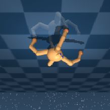
RAD                                      frame stack                                      2 frames

 Pendulum, Swingup
                                                                                                         (RAD)
                                                                latent flow                                                                               3 frames

                     Episode Return
                                                                (Flare)                                  latent stack + flow
                                                                                                         (Flare)
                                                                pixel flow                                                                                5 frames
                                                                                                         latent stack only
 Quadruped, Walk

                                                                                   Environment Step
                                      (a) pixel flow ablation                 (b) latent stacking ablation                     (c) frame count ablation

Figure 7: We perform 3 ablation studies: (a) Pixel flow ablation: we compare using pixel-level and
latent-level (Flare) differences. Flare is more stable and performs better. (b) Latent stack ablation: we
compare using latent stack with and without the latent flow. The latter performs significantly worse,
suggesting that the latent flow is crucial. (c) Frames count ablation: we test using different number
of frames for Flare.
learn effective policies on this task. We hypothesize that Flare trains more slowly with increased
frame count on Pendulum Swingup due to the presence of unnecessary information that the actor and
critic networks need to learn to ignore.

6                              C ONCLUSION
We propose Flare, an architecture for RL that explicitly encode temporal information by computing
flow in the latent space. In experiments, we show that in the state space, Flare can recover the optimal
performance with only state positions and no access to the state velocities. In the pixel space, Flare
improves upon the state-of-the-art model-free RL algorithms on the majority of selected tasks in the
DMControl and Atari suites, while matching in the remaining.

R EFERENCES
Artemij Amiranashvili, Alexey Dosovitskiy, Vladlen Koltun, and Thomas Brox. Motion perception
  in reinforcement learning with dynamic objects. In Conference on Robot Learning, pp. 156–168.
  PMLR, 2018.
Adrià Puigdomènech Badia, Bilal Piot, Steven Kapturowski, Pablo Sprechmann, Alex Vitvitskyi,
  Daniel Guo, and Charles Blundell. Agent57: Outperforming the atari human benchmark. In
 International Conference on Machine Learning, 2020.
Marc G Bellemare, Yavar Naddaf, Joel Veness, and Michael Bowling. The arcade learning environ-
 ment: An evaluation platform for general agents. Journal of Artificial Intelligence Research, 47:
 253–279, 2013.
Marc G Bellemare, Will Dabney, and Rémi Munos. A distributional perspective on reinforcement
 learning. arXiv preprint arXiv:1707.06887, 2017.
Christopher Berner, Greg Brockman, Brooke Chan, Vicki Cheung, Przemyslaw Debiak, Christy
  Dennison, David Farhi, Quirin Fischer, Shariq Hashme, Chris Hesse, et al. Dota 2 with large scale
  deep reinforcement learning. arXiv preprint arXiv:1912.06680, 2019.
Joao Carreira and Andrew Zisserman. Quo vadis, action recognition? a new model and the kinetics
  dataset. In proceedings of the IEEE Conference on Computer Vision and Pattern Recognition, pp.
  6299–6308, 2017.

                                                                                               8
Yevgen Chebotar, Mrinal Kalakrishnan, Ali Yahya, Adrian Li, S. Schaal, and S. Levine. Path integral
guided policy search. 2017 IEEE International Conference on Robotics and Automation (ICRA),
pp. 3381–3388, 2017.
Jeffrey Donahue, Lisa Anne Hendricks, Sergio Guadarrama, Marcus Rohrbach, Subhashini Venu-
gopalan, Kate Saenko, and Trevor Darrell. Long-term recurrent convolutional networks for visual
recognition and description. In Proceedings of the IEEE conference on computer vision and pattern
recognition, pp. 2625–2634, 2015.
Alexey Dosovitskiy, German Ros, Felipe Codevilla, Antonio Lopez, and Vladlen Koltun. Carla: An
open urban driving simulator. arXiv preprint arXiv:1711.03938, 2017.
Lasse Espeholt, Hubert Soyer, Remi Munos, Karen Simonyan, Volodymir Mnih, Tom Ward, Yotam
Doron, Vlad Firoiu, Tim Harley, Iain Dunning, et al. Impala: Scalable distributed deep-rl with
importance weighted actor-learner architectures. arXiv preprint arXiv:1802.01561, 2018.
Christoph Feichtenhofer, Haoqi Fan, Jitendra Malik, and Kaiming He. Slowfast networks for
video recognition. In Proceedings of the IEEE international conference on computer vision, pp.
6202–6211, 2019.
Meire Fortunato, Mohammad Gheshlaghi Azar, Bilal Piot, Jacob Menick, Ian Osband, Alex Graves,
Vlad Mnih, Remi Munos, Demis Hassabis, Olivier Pietquin, et al. Noisy networks for exploration.
arXiv preprint arXiv:1706.10295, 2017.
Tuomas Haarnoja, Aurick Zhou, Pieter Abbeel, and Sergey Levine. Soft actor-critic: Off-policy maxi-
mum entropy deep reinforcement learning with a stochastic actor. arXiv preprint arXiv:1801.01290,
2018.
Danijar Hafner, Timothy Lillicrap, Jimmy Ba, and Mohammad Norouzi. Dream to control: Learning
behaviors by latent imagination. arXiv preprint arXiv:1912.01603, 2019a.
Danijar Hafner, Timothy Lillicrap, Ian Fischer, Ruben Villegas, David Ha, Honglak Lee, and James
Davidson. Learning latent dynamics for planning from pixels. In International Conference on
Machine Learning, pp. 2555–2565. PMLR, 2019b.
Hado Hasselt. Double q-learning. Advances in neural information processing systems, 23:2613–2621,
2010.
Matteo Hessel, Joseph Modayil, Hado Van Hasselt, Tom Schaul, Georg Ostrovski, Will Dabney, Dan
Horgan, Bilal Piot, Mohammad Azar, and David Silver. Rainbow: Combining improvements in
deep reinforcement learning. arXiv preprint arXiv:1710.02298, 2017.
Divye Jain, Andrew Li, Shivam Singhal, Aravind Rajeswaran, Vikash Kumar, and Emanuel Todorov.
Learning Deep Visuomotor Policies for Dexterous Hand Manipulation. In International Conference
on Robotics and Automation (ICRA), 2019.
Shuiwang Ji, Wei Xu, Ming Yang, and Kai Yu. 3d convolutional neural networks for human action
recognition. IEEE transactions on pattern analysis and machine intelligence, 35(1):221–231,
2012.
Steven Kapturowski, Georg Ostrovski, John Quan, Remi Munos, and Will Dabney. Recurrent
experience replay in distributed reinforcement learning. In International conference on learning
representations, 2018.
A. Karpathy, G. Toderici, S. Shetty, T. Leung, R. Sukthankar, and L. Fei-Fei. Large-scale video
classification with convolutional neural networks. In 2014 IEEE Conference on Computer Vision
and Pattern Recognition, pp. 1725–1732, 2014.
Ilya Kostrikov, Denis Yarats, and Rob Fergus. Image augmentation is all you need: Regularizing
deep reinforcement learning from pixels. arXiv preprint arXiv:2004.13649, 2020.
Michael Laskin, Kimin Lee, Adam Stooke, Lerrel Pinto, Pieter Abbeel, and Aravind Srinivas.
Reinforcement learning with augmented data. arXiv preprint arXiv:2004.14990, 2020a.
9Michael Laskin, Aravind Srinivas, and Pieter Abbeel. Curl: Contrastive unsupervised representations
for reinforcement learning. Proceedings of the 37th International Conference on Machine Learning,
Vienna, Austria, PMLR 119, 2020b. arXiv:2004.04136.
Timothy P. Lillicrap, Jonathan J. Hunt, Alexander Pritzel, Nicolas Heess, Tom Erez, Yuval Tassa,
David Silver, and Daan Wierstra. Continuous control with deep reinforcement learning. In ICLR,
2016.
Kendall Lowrey, Svetoslav Kolev, Jeremy Dao, Aravind Rajeswaran, and Emanuel Todorov. Rein-
forcement learning for non-prehensile manipulation: Transfer from simulation to physical system.
In IEEE SIMPAR, 2018.
Volodymyr Mnih, Koray Kavukcuoglu, David Silver, Andrei A Rusu, Joel Veness, Marc G Bellemare,
Alex Graves, Martin Riedmiller, Andreas K Fidjeland, Georg Ostrovski, et al. Human-level control
through deep reinforcement learning. Nature, 518(7540):529–533, 2015.
Volodymyr Mnih, Adria Puigdomenech Badia, Mehdi Mirza, Alex Graves, Timothy Lillicrap, Tim
Harley, David Silver, and Koray Kavukcuoglu. Asynchronous methods for deep reinforcement
learning. In International conference on machine learning, pp. 1928–1937, 2016.
OpenAI, Marcin Andrychowicz, Bowen Baker, Maciek Chociej, Rafał Józefowicz, Bob McGrew,
Jakub Pachocki, Arthur Petron, Matthias Plappert, Glenn Powell, Alex Ray, Jonas Schneider,
Szymon Sidor, Josh Tobin, Peter Welinder, Lilian Weng, and Wojciech Zaremba. Learning
dexterous in-hand manipulation. CoRR, abs/1808.00177, 2018.
John Quan and Georg Ostrovski. DQN Zoo: Reference implementations of DQN-based agents, 2020.
URL http://github.com/deepmind/dqn_zoo.
Aravind Rajeswaran, Vikash Kumar, Abhishek Gupta, Giulia Vezzani, John Schulman, Emanuel
Todorov, and Sergey Levine. Learning Complex Dexterous Manipulation with Deep Reinforcement
Learning and Demonstrations. In Proceedings of Robotics: Science and Systems (RSS), 2018.
Manolis Savva, Abhishek Kadian, Oleksandr Maksymets, Yili Zhao, Erik Wijmans, Bhavana Jain,
Julian Straub, Jia Liu, Vladlen Koltun, Jitendra Malik, et al. Habitat: A platform for embodied ai
research. In Proceedings of the IEEE International Conference on Computer Vision, pp. 9339–9347,
2019.
Tom Schaul, John Quan, Ioannis Antonoglou, and David Silver. Prioritized experience replay. arXiv
preprint arXiv:1511.05952, 2015.
John Schulman, Filip Wolski, Prafulla Dhariwal, Alec Radford, and Oleg Klimov. Proximal policy
optimization algorithms. arXiv preprint arXiv:1707.06347, 2017.
Max Schwarzer, Ankesh Anand, Rishab Goel, R Devon Hjelm, Aaron Courville, and Philip Bachman.
Data-efficient reinforcement learning with momentum predictive representations. arXiv preprint
arXiv:2007.05929, 2020.
David Silver, Aja Huang, Christopher J. Maddison, Arthur Guez, Laurent Sifre, George van den
Driessche, Julian Schrittwieser, Ioannis Antonoglou, Veda Panneershelvam, Marc Lanctot, Sander
Dieleman, Dominik Grewe, John Nham, Nal Kalchbrenner, Ilya Sutskever, Timothy Lillicrap,
Madeleine Leach, Koray Kavukcuoglu, Thore Graepel, and Demis Hassabis. Mastering the game
of go with deep neural networks and tree search. Nature, 529:484–503, 2016. URL http:
//www.nature.com/nature/journal/v529/n7587/full/nature16961.html.
David Silver, Julian Schrittwieser, Karen Simonyan, Ioannis Antonoglou, Aja Huang, Arthur Guez,
Thomas Hubert, Lucas Baker, Matthew Lai, Adrian Bolton, Yutian Chen, Timothy Lillicrap, Fan
Hui, Laurent Sifre, George Driessche, Thore Graepel, and Demis Hassabis. Mastering the game of
go without human knowledge. Nature, 550:354–359, 10 2017. doi: 10.1038/nature24270.
Karen Simonyan and Andrew Zisserman. Two-stream convolutional networks for action recognition
in videos. In Advances in neural information processing systems, pp. 568–576, 2014.
Khurram Soomro, Amir Roshan Zamir, and Mubarak Shah. Ucf101: A dataset of 101 human actions
classes from videos in the wild. arXiv preprint arXiv:1212.0402, 2012.
10Adam Stooke, Kimin Lee, Pieter Abbeel, and Michael Laskin. Decoupling representation learning
from reinforcement learning, 2020.
Richard Sutton and Andrew Barto. Reinforcement Learning: An Introduction. MIT Press, 1998.
Yuval Tassa, Yotam Doron, Alistair Muldal, Tom Erez, Yazhe Li, Diego de Las Casas, David Budden,
Abbas Abdolmaleki, Josh Merel, Andrew Lefrancq, et al. Deepmind control suite. arXiv preprint
arXiv:1801.00690, 2018.
Emanuel Todorov, Tom Erez, and Yuval Tassa. Mujoco: A physics engine for model-based control.
In IROS, 2012.
Du Tran, Lubomir Bourdev, Rob Fergus, Lorenzo Torresani, and Manohar Paluri. Learning spa-
tiotemporal features with 3d convolutional networks. In Proceedings of the IEEE international
conference on computer vision, pp. 4489–4497, 2015.
Oriol Vinyals, Igor Babuschkin, Wojciech M. Czarnecki, Michaël Mathieu, Andrew Dudzik, Junyoung
Chung, David H. Choi, Richard Powell, Timo Ewalds, Petko Georgiev, Junhyuk Oh, Dan Horgan,
Manuel Kroiss, Ivo Danihelka, Aja Huang, Laurent Sifre, Trevor Cai, John P. Agapiou, Max
Jaderberg, Alexander S. Vezhnevets, Rémi Leblond, Tobias Pohlen, Valentin Dalibard, David
Budden, Yury Sulsky, James Molloy, Tom L. Paine, Caglar Gulcehre, Ziyu Wang, Tobias Pfaff,
Yuhuai Wu, Roman Ring, Dani Yogatama, Dario Wünsch, Katrina McKinney, Oliver Smith, Tom
Schaul, Timothy Lillicrap, Koray Kavukcuoglu, Demis Hassabis, Chris Apps, and David Silver.
Grandmaster level in starcraft ii using multi-agent reinforcement learning. Nature, 575(7782):
350–354, 2019. doi: 10.1038/s41586-019-1724-z. URL https://doi.org/10.1038/
s41586-019-1724-z.
Aaron Walsman, Yonatan Bisk, Saadia Gabriel, Dipendra Misra, Yoav Artzi, Yejin Choi, and Dieter
Fox. Early Fusion for Goal Directed Robotic Vision. In International Conference on Intelligent
Robots and Systems (IROS), 2019.
Xiaolong Wang, Ross Girshick, Abhinav Gupta, and Kaiming He. Non-local neural networks. In
Proceedings of the IEEE conference on computer vision and pattern recognition, pp. 7794–7803,
2018.
Ziyu Wang, Tom Schaul, Matteo Hessel, Hado Hasselt, Marc Lanctot, and Nando Freitas. Dueling
network architectures for deep reinforcement learning. In International conference on machine
learning, pp. 1995–2003, 2016.
Denis Yarats, Amy Zhang, Ilya Kostrikov, Brandon Amos, Joelle Pineau, and Rob Fergus. Im-
proving sample efficiency in model-free reinforcement learning from images. arXiv preprint
arXiv:1910.01741, 2019.
H. Zhu, A. Gupta, A. Rajeswaran, S. Levine, and V. Kumar. Dexterous manipulation with deep
reinforcement learning: Efficient, general, and low-cost. 2019 International Conference on
Robotics and Automation (ICRA), pp. 3651–3657, 2019.
11A A PPENDIX
A.1 BACKGROUND
Soft Actor Critic (SAC) (Haarnoja et al., 2018) is an off-policy actor-critic RL algorithm for
continuous control with an entropy maximization term augmented to its score function to encourage
exploration. SAC learns a policy network πψ (at |ot ) and critic networks Qφ1 (ot , at ) and Qφ2 (ot , at )
to estimate state-action values. The critic Qφi (ot , at ) is optimized to minimize the (soft) Bellman
residual error: h 2 i
LQ (φi ) = Eτ ∼B Qφi (ot , at ) − (rt + γV (ot+1 )) , (1)
where r is the reward, γ the discount factor, τ = (ot , at , ot+1 , rt ) is a transition sampled from replay
buffer B, and V (ot+1 ) is the (soft) target value estimated by:
V (ot+1 ) = min Qφ̄i (ot+1 , at+1 ) − α log πψ (at+1 |ot+1 )] , (2)
i
where α is the entropy maximization coefficient. For stability, in eq. 2, Qφ̄i is the exponential moving
average of Qφi ’s over training iterations. The policy πψ is trained to maximize the expected return
estimated by Q together with the entropy term
Lπ (ψ) = −Eat ∼π [min Qφi (ot , at ) − α log πψ (at |ot )], (3)
i
where α is also a learnable parameter.
Reinforcement Learning with Augmented Data (RAD) (Laskin et al., 2020a) is a recently proposed
training technique. In short, RAD pre-processes raw pixel observations by applying random data
augmentations, such as random translation and cropping, for RL training. As simple as it is, RAD
has taken many existing RL algorithms, including SAC, to the next level. For example, on many
DMControl (Tassa et al., 2018) benchmarks, while vanilla pixel-based SAC performs poorly, RAD-
SAC—i.e. applying data augmentation to pixel-based SAC—achieves state-of-the-art results both
in sample efficiency and final performance. In this work, we refer RAD to RAD-SAC and the
augmentation used is random translation.
Rainbow DQN is an extension of the Nature Deep Q Network (DQN) (Mnih et al., 2015), which
combines multiple follow-up improvements of DQN to a single algorithm (Hessel et al., 2017). In
summary, DQN (Mnih et al., 2015) is an off-policy RL algorithm that leverages deep neural networks
(DNN) to estimate the Q value directly from the pixel space. The follow-up works Rainbow DQN
bring together to enhance the original DQN include double Q learning (Hasselt, 2010), prioritized
experience replay (Schaul et al., 2015), dueling network (Wang et al., 2016), noisy network (Fortunato
et al., 2017), distributional RL (Bellemare et al., 2017) and multi-step returns (Sutton & Barto, 1998).
Rainbow DQN is one of the state-of-the-art RL algorithms on the Atari 2600 benchmark (Bellemare
et al., 2013). We thus adopt an official implementation of Rainbow (Quan & Ostrovski, 2020) as our
baseline to directly augment Flare on top.
A.2 E NVIRONMENTS AND E VALUATION M ETRICS
The DeepMind Control Suite (DMControl) (Tassa et al., 2018), based on MuJoCo (Todorov et al.,
2012), is a commonly used benchmark for continuous control from pixels. Prior works such as
DrQ (Kostrikov et al., 2020) and RAD (Laskin et al., 2020a) have made substantial progress on
this benchmark and closed the gap between state-based and pixel-based efficiency on the simpler
environments in the suite, such as Reacher Easy, Ball-in-cup Catch, Finger Spin, Walker Walk,
Cheetah Run, Cartpole Swingup. However, current pixel-based RL algorithms struggle to learn
optimal policies efficiently in more challenging environments that feature partial observability, sparse
rewards, or precise manipulation. In this work, we study more challenging tasks from the suite
to better showcase the efficacy of our proposed method. The 5 environments, listed in Figure 8,
include Walker Run (requires maintaining balance with speed), Quadruped Walk (partially observable
agent morphology), Hopper Hop (locomotion with sparse rewards), Finger Turn-hard (precise
manipulation), and Pendulum Swingup (torque control with sparse rewards). For evaluation, we
benchmark performance at 500K and 1M environment steps and compare against RAD.
The Atari 2600 Games (Bellemare et al., 2013) is another highly popular RL benchmark. Recent
efforts have let to a range of highly successful algorithms (Espeholt et al., 2018; Hessel et al., 2017;
12Quadruped Walk Hopper Hop Pendulum Swingup Walker Run Finger Turn Hard
Figure 8: We choose the following environments for our main experiments – (i) quadruped walk,
which requires coordination of multiple joints, (ii) hopper hop, which requires hopping while
maintaining balance, (iii) pendulum swingup, an environment with sparse rewards, (iv) walker run,
which requires the agent to maintain balance at high speeds, and (v) finger turn hard, which requires
precise manipulation of a rotating object. These environments are deemed challenging because prior
state-of-the-art model-free pixel-based methods (Laskin et al., 2020b; Kostrikov et al., 2020; Laskin
et al., 2020a) either fail to reach the asymptotic performance of state SAC or learn less efficiently.
Kapturowski et al., 2018; Hafner et al., 2019a; Badia et al., 2020) to solve Atari games directly from
pixel space. A representative state-of-the-art is Rainbow DQN (see Section A.1). We adopt the official
Rainbow DQN implementation (Quan & Ostrovski, 2020) as our baseline. Then we simply modify
the model architecture to incorporate Flare while retaining all the other default settings, including
hyperparameters and preprocessing. To ensure comparable model capacity, the Flare network halves
the number of convolutional channels and adds a bottleneck FC layer to reduce latent dimension
before entering the Q head (code in the Supplementary Materials). We evaluate on a diverse subset of
Atari games at 50M training steps, namely Assault, Breakout, Freeway, Krull, Montezuma Revenge,
Seaquest, Up n Down and Tutankham, to assess the effectiveness of Flare.
A.3 C OMPARE F LARE WITH DQN VARIANTS ON ATARI
Flare Rainbow Rainbow† Prioritized† QR DQN† IQN†
Assault 12724±1107 15229±2061 13194±4348 10163±1558 10215±1255 11903±1251
Breakout 345±22 280±18 366±20 359±33 450±29 492±86
Berzerk 2049±421 1636±598 3151±537 986±98 896±98 946±48
Defender 86982±29214 44694±3984 52419±4481 13750±4182 32320±8997 33767±3643
Montezuma 1668±1055 900±807 80±160 0±0 0±0 0±0
Seaquest 13901±8085 24090±12474 5838±2450 7436±1790 14864±3625 16866±4539
Phoenix 60974±18044 16992±3295 82234±33388 10667±3142 41866±3673 35586±3510
Tutankham 248±20 247±11 214±24 168±22 171±30 216±34
Table 3: Evaluation on 8 benchmark Atari games at 100M training steps over 5 seeds. † directly taken from
DQN Zoo repository and the rest are collected from our experiments.
13A.4 I MPLEMENTATION D ETAILS FOR P IXEL - BASED E XPERIMENTS
Hyperparameter Value
Augmentation Random Translate
Observation size (100, 100)
Augmented size (108, 108)
Replay buffer size 100000
Initial steps 10000
Training environment steps 1.5e6 pendulum swingup
2.5e6 others
Batch size 128
Stacked frames 2 pendulum swingup
3 others
Action repeat 2 walker run, hopper hop
4 others
Camera id 2 quadruped, walk
0 others
Evaluation episode length 10
Hidden units (MLP) 1024
Number of layers (MLP) 2
Optimizer Adam
(β1 , β2 ) → (fCN N , πψ , Qφ ) (.9, .999)
(β1 , β2 ) → (α) (.5, .999)
Learning Rate (πψ , Qφ ) 2e − 4
Learning Rate (fCN N ) 1e − 3
Learning Rate (α) 1e − 4
Critic target update frequency 2
Critic EMA τ 0.01
Encoder EMA τ 0.05
Convolutional layers 4
Number of CNN filters 32
Latent dimension 64
Non-linearity ReLU
Discount γ 0.99
Initial Temperature 0.1
A.5 I MPLEMENTATION D ETAILS FOR S TATE - BASED M OTIVATION E XPERIMENTS
Hyperparameter Value
Replay buffer size 2000000
Initial steps 5000
Batch size 1024
Stacked frames 4 Flare, Stack SAC;
1 otherwise
Action repeat 1
Evaluation episode length 10
Hidden units 1024
Number of layers 2
Optimizer Adam
(β1 , β2 ) → (fCN N , πψ , Qφ ) (.9, .999)
(β1 , β2 ) → (α) (.9, .999)
Learning Rate (πψ , Qφ ) 1e − 4
Learning Rate (α) 1e − 4
Critic target update frequency 2
Critic EMA τ 0.01
Non-linearity ReLU
Discount γ 0.99
Initial Temperature 0.1
14A.6 I NTERPRETING FLARE FROM A T WO - STREAM P ROSPECTIVE
Let fCNN and o0t be the pixel encoder and the augmented observation in Flare. Then, zt = fCNN (o0t )
denotes the latent encoding for a frame at time t. By computing the latent flow δt = zt − zt−1 , Flare
essentially approximates ∂z
∂t via backward finite difference. Then following chain rule, we have
t
∂z ∂z ∂o0 fCNN (o0 )
= 0· = · dense optical flow
∂t ∂o ∂t ∂o0
indicating that Flare eventually uses dense optical flow by propagating it through the derivative
of the trained encoder. While the two-stream architecture trains a spatial stream CNN from RGB
channels and a temporal stream from optical flow separately, Flare can be interpreted as training one
spatial stream encoder from the RL objective and approximate the temporal stream encoder with its
derivative.
15You can also read