SafeBuild: Risk-Based Analysis of Overhead Electric Distribution Facilities
←
→
Page content transcription
If your browser does not render page correctly, please read the page content below

SafeBuild: Risk-Based Analysis of Overhead
                 Electric Distribution Facilities
                                                           Jennifer Lew
                                                Palos Verdes Peninsula High School
                                                    Rolling Hills Estates, USA
                                                     jennlew2004@gmail.com

   Abstract—California has experienced increasingly adverse ef-          improves upon existing software: for any wind gust inputted by
fects from the failure of overhead electric infrastructure. In           the user, SafeBuild calculates the probability that the pole can
2011, in the San Gabriel Valley, 248 utility poles broke, causing        successfully withstand the wind gust. SafeBuild calculates the
an outage to 440,000 customers for up to a week. In 2018, a
component on a transmission tower broke, igniting the Camp               stress on poles using large deflection finite element analysis.
Fire, which destroyed 18,804 buildings and killed 85 civilians.          SafeBuild then calculates the probability of failure of the
The cause of these incidents can be ascribed, in part, to deficient      pole using z-scores based on material median strengths and
methods in accurately capturing the probability that a given pole,       coefficients of variation. SafeBuild can also calculate the
conductor, or other component can withstand windy conditions             increase in conductor tension due to external forces, which will
without breaking. Existing software and methodology do not
account for material strength variability or even calculate a            allow users to calculate the probability of failure of structural
possibility of failure based on known local wind speeds. The             members, e.g. wood crossarms. Note that while SI units is the
current research believes that it can correct these shortcomings         staple in most fields, SafeBuild uses US Customary Units, as
by introducing a program – SafeBuild – that provides the                 this is the industry standard.
probability that a structure can withstand any given wind gust.
SafeBuild calculates the stress on poles and conductors using                                  II. M ETHODOLOGY
large deflection finite element analysis. SafeBuild calculates the
                                                                         A. Pole Deformation due to Wind Loading
probability of failure of any component using z-scores based
on material median strengths and coefficients of variation. The             In windy conditions, wood poles will deflect due to wind
research successfully created a program that is user-friendly and        loading on the exposed surfaces of the wood pole and the
accurate. SafeBuild fits into the bigger picture of utility safety and   facilities it supports. One of the greatest forces on the pole
wildfire prevention by allowing users to design poles to withstand
a wind gust to any desired confidence level.                             results from wind blowing on overhead conductors [1]:
   Index Terms—beam element, cable element, large deformation,                        Fwind,conductor = QKz Kd GCf V 2 A              (1)
utility pole, risk analysis, wind loading
                                                                         In (1), Q is the air density factor, Kz is the velocity pres-
                        I. I NTRODUCTION                                 sure exposure coefficient accounting for the increase in wind
   In California, the failure of electric utility infrastructure has     pressure with height above ground, Kd is the directionality
increasingly led to adverse outcomes. From 2017 to 2019,                 factor accounting for wind direction, G is the gust effect factor
one utility in California ignited 49 wildfires. Of these fires,          accounting for spatial averaging, Cf is the drag coefficient
the 2018 Camp Fire alone destroyed 18,804 buildings and                  of the conductor, and V is the wind gust in miles per hour.
killed 85 civilians. In these cases and others, the cause of             Inputting the necessary variables into (1) will yield a point
the incident can be attributed in some part to the failure of            force on the pole in units of lbf. Due to forces such as
the facilities to withstand known local wind speeds. In utility          those described in (1), a pole will deflect; when this occurs,
pole design, most commercial software will calculate a pole              the weight of the supported facilities - such as conductors,
safety factor by taking the pole’s bending moment resistance             cables, and transformers - will cause the pole to deflect
and dividing that by the bending moment due to a reference               even more via secondary P-∆ effects. Once the deflection
wind load. However, the drawback of this approach is that                of the pole is determined, the bending moment along the
there is no agreed upon method for translating a safety factor           pole can be calculated and compared to the bending moment
into a wind speed; indeed, there is not even agreement on                resistance along the pole. The current research uses finite
the definition of the term safety factor. Further, the software          element analysis [2] to calculate the pole’s deflection, wherein
calculates the bending moment resistance of the pole using the           the pole is modeled as a series of elements [3]. Figure 1 shows
median wood fiber strength; as a result, there is a 50% chance           an example of a utility pole modeled using three elements,
that the pole safety factor is less than the calculated result. In       which is numbered sequentially starting with Element 1 at
sum, a clear result such as “this wood pole can withstand a 112          the base. Using n to denote the index, we note that every
mile per hour wind gust with a 95% probability of success”               Element n has, at its tip, a node n (with the remaining node
is not achievable via existing software. The current research            0 representing the base of the pole at ground level). At each
has developed a structural design software – SafeBuild – that            node n, a horizontal force Fy,n and a vertical force Fx,n can be
As the pole bends, the base of each element rotates. For an
Element n, the rotation matrix is given as follows:
cosφn−1 −sinφn−1 0 0 0 0
sinφn−1 cosφn−1 0 0 0 0
0 0 1 0 0 0
λn =
(4)
0 0 0 cosφn−1 −sinφn−1 0
0 0 0 sinφn−1 cosφn−1 0
0 0 0 0 0 1
The global element stiffness matrix, which accounts for the
aforementioned rotation, can then by calculated as follows:
kn,global = λn · kn · λn T (5)
Fig. 1. Finite element representation of a utility pole.
The global element stiffness matrices for all the elements can
then be combined to form a global stiffness matrix K, as
applied, where the orientation of the x-axis and y-axis has been shown in Fig. 2. Next, the force matrix captures the horizontal
reversed to maintain the convention used in beam bending. force, vertical force, and moment applied at all the nodes.
After forces are applied, the pole will deflect. At each node n, Assuming that the pole is composed of m elements, the force
the horizontal deflection with respect to the base of the pole is matrix is given by:
δy,n , the vertical deflection with respect to its undeformed state
Fx,1
is δx,n (not shown in Figure 1), and the angle of deflection
with respect to vertical is denoted as φn . As shown in Figure
Fy,1
1, the horizontal and vertical deflections can also be broken
down to an element level; that is to say, the deflection of
Mθ,1
an Element n can be found by calculating the deflection at
..
node n with respect to node n − 1. These deflections, which F =
.
(6)
we call element horizontal and vertical deflections, are given
by δy,elem n and δx,elem n , respectively. For Element 1, the Fx,m
element stiffness matrix is given as follows:
Fy,m
AE1
0 0
L1
Mθ,m
12EI1 −6EI1
k1 = 0 L1 3 L1 2
(2)
In (6), Mθ,n represents the moment applied at node n, if any.
−6EI1 4EI1
The displacement matrix, which captures the deflections at all
0 L1 2 L1 the nodes, is given as follows:
In (2), AE1 represents the cross-sectional area of Element 1 δx1
multiplied by the modulus of elasticity of Element 1 and is
in units of lb, EI1 represents the flexural rigidity of Element δy1
1 in lb-f t2 , and L1 represents the length of Element 1 in ft.
The element stiffness matrix for each subsequent element is φ1
given as follows: ..
.
d= (7)
−AEn
AEn
Ln 0 0 Ln 0 0
δx,m
12EIn 6EIn −12EIn 6EIn
0 Ln 3 Ln 2
0 Ln 3 Ln 2
δy,m
6EIn 4EIn −6EIn 2EIn
0 Ln 2 Ln 0 Ln 2 Ln
kn = (3)
−AEn
0 0 AEn
0 0 φm
Ln Ln
The values in the displacement matrix d can be solved using
−12EIn −6EIn 12EIn −6EIn
0 Ln 3 Ln 2
0 Ln 3 Ln 2 the equation:
0 6EIn 2EIn
0 −6EIn 4EIn d = K −1 F (8)
Ln 2 Ln Ln 2 Ln
In (8), the calculated horizontal deflection values δy,n is
considered accurate; however, the calculated vertical deflection
values δx,n is considered to have inaccurately captured the
downward deflection of the elements. However, the values
for δx,n can be corrected. Looking at a single element, the
horizontal deflection of the element is given by:
δy,elem n = δy,n − δy,n−1 (9)
The value in (9) can then be substituted into the following
equation to yield the corrected vertical downward deflection
on a per element basis:
s 2
δy,elem n
δx,elem n = Ln − Ln 2 − (10)
0.91879
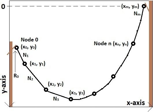
Fig. 3. Model of the conductor using finite elements.
The accuracy of the process in (9) and (10) was validated
against known beam bending experiments [4]. Once the deflec-
tion curve of the pole is fully known, the bending moment BM B. Conductor Deformation due to External Forces
in lb-ft at any point along the pole can be found. If we assume As shown in Fig. 3, a conductor can be modeled using m
that BM is calculated at the pole’s groundline (commonly elements, where each element can be numbered sequentially
the weakest point of a typical distribution pole), then BM starting with Element 1 at the left attachment point. The con-
will need to be compared to the bending moment resistance ductor’s left and right attachment points will be Node 0 with
BMres at groundline. The bending moment resistance of the coordinate (x0 , y0 ) and Node m with coordinate (xm , ym ),
pole, in lb-ft, at its groundline is given as follows: respectively. Using n to denote the index, an Element n has an
axial force of Nn and a length of Ln . As an initial condition,
BMres = 0.000264Cg 3 (1 − z · CV ) Fb,med (11) the coordinates of the nodes should represent the curvature
of the conductor at the time of installation. The length Ln of
In (11), Cg represents the pole’s groundline circumference in element n is given as follows:
inches, z is the z-score, CV is the coefficient of variation of q
2 2
the wood species, typically given as 0.2 [5], and Fb,med is Ln = (xn − xn−1 ) + (yn − yn−1 ) (12)
the wood’s median fiber strength in psi. The value of z in
The axial force of Element 1 can be found as follows:
(11) shall be adjusted until BMres just equals the bending
moment BM at the same point. Then, a table of z-scores can R0 L1
N1 = (13)
then be referenced to determine the probability that the pole y1 − y0
can withstand the bending moment imposed by the wind gust. In (13), R0 is the reaction force at Node 0 in the conductor’s
initial condition, which is equivalent to the vertical component
of tension at the left attachment point. The axial force of every
element except the first element is given by:
xn−1 −xn−2
Nn−1 · Ln−1
Nn = xn −xn−1 (14)
Ln
The direction cosine for Element n is given by:
xn − xn−1
cn = q (15)
2 2
(xn − xn−1 ) + (yn − yn−1 )
The direction sine for Element n is given by:
yn − yn−1
sn = q (16)
2 2
(xn − xn−1 ) + (yn − yn−1 )
The stiffness matrix for Element n is given by:
ka,n −ka,n
Fig. 2. Global stiffness matrix.
kn = (17)
−ka,n ka,n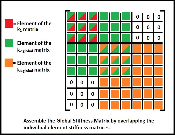
where: TABLE I
" # " # CONDUCTORS AND EQUIPMENT SUPPORTED ON THE
EA cn 2 cn sn Nn (1 − cn 2 ) −cn sn EXAMPLE POLE
ka,n = + (18)
Ln cn sn sn 2 Ln −cn sn (1 − sn 2 ) Conductor Attachments
Left Right Diameter Heightb Weight No. Type
The element stiffness matrices can be combined together to Span Span or
Lengtha Length Density
create a global stiffness matrix K via the same method shown 400 ft 300 ft 0.25 in 44 ft 0.2 lb/ft 3 Wire
in Fig. 2. At each Node n, forces can be applied that represent 400 ft 300 ft 0.50 in 33 ft 0.5 lb/ft 1 Wire
external forces such as a falling tree branch. If we use Fx,n 400 ft 300 ft 0.75 in 24.5 ft 1 lb/ft 1 TV
cable
and Fy,n to denote the forces on Node n, then the force matrix 400 ft 300 ft 0.50 in 20.3 ft 0.5 lb/ft 1 Phone
will be as follows: cable
Equipment Attachments
Fx,1 0 0 0 37.5 ft 600 lb 1
a Length of the conductor span to the left or right of the pole.
XFMR
b Attachment height of the conductor or equipment on the pole.
Fy,1
..
F =
.
(19)
If the out-of-balance forces are significant, then a further nodal
Fx,m−1 displacement can be found as follows:
Fy,m−1 q = K −1 ∆F (24)
It is expected that values in (19) are sufficiently large to ensure Using (24), the nodal coordinates can be updated as many
that K does not reach singularity. With this understanding, the times as necessary to achieve accuracy. The final axial forces
forces in (19) will cause the conductor to deform such that the in all the elements will be given by (13) and (14).
coordinates of a Node n will change. This is captured in the III. R ESULTS
nodal displacement matrix, q:
A. Wind Loading of a Utility Pole
∆x1 A utility pole is wind loaded in three trials. The Class 4 pole
has a length of 50 feet, with 6 feet underground. The facilities
∆y1
supported on the pole (e.g. conductors, cables, transformers),
..
shown in Table I, is identical for all trials. For Trial 1, the pole
q=
.
(20)
is Red Cedar (median fiber strength of 5800 psi) and the wind
gust is 112 mph. The results in Fig. 4 show that the pole has
∆xm−1
an 8.69% chance of withstanding the wind. For Trial 2, the
∆ym−1 pole is Douglas Fir (median fiber strength of 8000 psi) and the
wind gust remains 112 mph. The results in Fig. 5 show that
Notice that (19) and (20) do not include forces and displace- the pole has a 67.36% chance of withstanding the wind. For
ment values, respectively, for the attachment points at Node Trial 3, the pole is Douglas Fir and the wind gust is lowered to
0 and Node m as these points are fixed. The displacement 92 mph. The results in Fig. 6 show that the pole has a 97.13%
matrix q can then be calculated as follows: chance of withstanding the wind.
q = K −1 F (21)
Solving for (21) is just the first step in solving for the
deformation of the conductor due to external forces. Once q
is known, all the nodal coordinates (xn , yn ) need be updated.
Once this is done, any out-of-balance force can be found by
applying force equilibrium at the nodes. For example, the out-
of-balance force in the x-direction at Node 2 can be found as
follows:
−N2 (x2 − x1 ) N3 (x3 − x2 )
∆Fx,2 = + + Fx,2 (22)
L2 L3
The out-of-balance force in the y-direction at Node 2 can be
found as follows:
−N2 (y2 − y1 ) N3 (y3 − y2 ) Fig. 4. Trial 1: The pole has an 8.69% chance of not breaking.
∆Fy,2 = + + Fy,2 (23)
L2 L3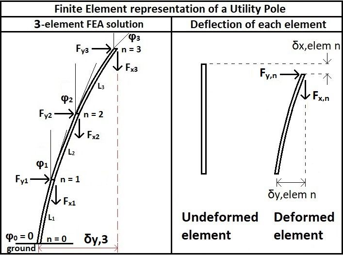
Fig. 5. Trial 2: The pole has a 67.36% chance of not breaking.
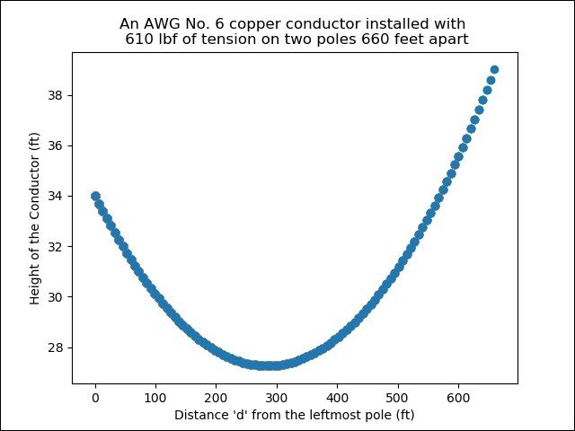
Fig. 7. Conductor in installation stage.
Fig. 6. Trial 3: The pole has a 97.13% chance of not breaking.
B. Tree Branch Falling on an Overhead Conductor
Assume an American Wire Gauge (AWG) No. 6 copper
conductor is supported by poles installed 660 feet apart. The Fig. 8. Tree branch falling on conductor.
conductor height on the left and right pole is 34 feet and 39
feet, respectively. The installation tension is 610 lbf. This is
SafeBuild can also prevent utility poles in low wind areas from
shown in Fig. 7. Assume a 25 lb tree branch falls 30 ft onto
being overbuilt, thereby saving money.
the conductor at a distance d = 330 ft, as shown in Fig. 8.
Per SafeBuild, this produces an average impact force of 100.5 ACKNOWLEDGMENT
lbf, which will cause the tension in the conductor to increase The author thanks her advisor, Derek Fong, PE, Senior
to 1004.5 lbf. As the tensile strength of AWG No. 6 medium Utilities Engineer Supervisor at the California Public Utilities
hard drawn copper is 1000 lbf, the conductor will break. Commission, for his technical guidance, editing, and direction.
IV. C ONCLUSION R EFERENCES
Current design tools calculate a pole safety factor based [1] M. M. Alam, B. E. Tokgoz, and S. Hwang, “Framework for measuring
the resilience of utility poles of an electric power distribution network,”
on a reference wind load. However, safety factors cannot be Int. J. Disaster Risk Sci., vol. 10, pp. 270–281, 2019.
easily translated to a wind speed. Instead of generating a safety [2] N. Kim and B. V. Sankar, Introduction to Finite Element Analysis and
factor, SafeBuild calculates the probability that a pole can Design. New York, NY: John Wiley & Sons, 2009.
[3] B. L. Barton, M. S. Shetty, V. Birman, and L. R. Dharani, “Tapered
withstand a given wind gust. Thus, SafeBuild can be used to cylindrical cantilever beam retrofitted with steel reinforced polymer or
design an electric system using a risk-based methodology. For grout,” Composites: Part B, vol. 42, pp. 207–216, 2011.
example, an engineer can use SafeBuild to design all poles [4] C. Neipp and A. Belendez, “Large and small deflections of a cantilever
beam,” Eur. J. Phys., vol. 23, pp. 371–379, May 2002.
to have a 99% probability of withstanding the greatest 50- [5] R. W. Wolfe and R. O. Kluge, “Designated fiber stress for wood
year wind gust in a given area. SafeBuild can prevent utility poles,” U.S. Department of Agriculture, Forest Service, Forest Products
poles from being underbuilt, thereby enhancing public safety; Laboratory, Madison, WI, USA, Gen. Tech. Rep. FPL-GTR-158, 2005.
You can also read