Scarcity, Work, and Choice - ECONOMIC THEORY 1A WEEK 3 - Michael Sachs

ECONOMIC THEORY 1A WEEK 3

Scarcity, Work, and Choice

2
Outline

 This lecture covers Chapter 3 of “The Economy” textbook. In this
 chapter, we will use economic models to:
 1. Investigate decision making under scarcity: How do we meet
 our objectives given our limited means?
 2. Model three different contexts in which different people
 decide how long to spend working, when facing a trade-off:
 A student, a farmer, and a wage earner.
 3. Provide an explanation for why working hours have changed
 over time: Why does it differ between countries?

3
Remember to use the Glossary section on www.core-econ.org

▪ https://core-econ.org/the-economy/book/text/50-02-glossary.html#glossary

scarcity
▪ A [scarce good is a] good that is valued, and for which there is an opportunity cost of
 acquiring more.
opportunity cost
▪ When taking an action implies forgoing the next best alternative action, this is the net
 benefit of the foregone alternative.
economic cost
▪ The out-of-pocket cost of an action, plus the opportunity cost.

 In economics, knowing and understanding definitions is
 VERY important!

4
Introduction

▪ Decision making under scarcity is a common problem because we
 usually have limited means available to meet our objectives.
▪ Economists model these situations, first by defining all of the
 feasible actions, then evaluating which of these actions is best,
 given the objectives.
▪ A model of decision making under scarcity can be applied to the
 question of how much time to spend working (or studying) when
 facing a trade-off between more free time and more income (a
 higher grade).

5

Labour and Production
The production function, preferences,
and the feasible set

6
A note on ceteris paribus

▪ In economics, you will often see the Latin phrase “ceteris paribus.”
▪ From the glossary:
 ‒ The literal meaning of the expression is ‘other things equal’. In an
 economic model it means an analysis ‘holds other things
 constant.’
 ‒ Economists often simplify analysis by setting aside things that are
 thought to be of less importance to the question of interest.

 In building our models in this chapter, we will make many
 simplifying assumptions which help us “see more by looking at less.”

7
How many hours to spend studying?

▪ As a student, you make a choice every day: how many hours to
 spend studying.
▪ Many factors may influence your choice: how much you enjoy your
 work, how difficult you find it, how much work your friends do, and
 so on.
▪ Part of the motivation to devote time to studying comes from your
 belief that the more time you spend studying, the higher the grade
 you will be able to obtain at the end of the course.
▪ We will construct a simple model of a student’s choice of how many
 hours to work, based on the assumption that the more time spent
 working, the better the final grade will be, ceteris paribus.
▪ The first building block of this model is called the production
 function.

8
The Production Function

▪ Recall from Unit 2 that a production function is a graphical or
 mathematical expression that gives the maximum output for a
 given amount or combination of input(s).
▪ A student’s production
 function translates the
 number of hours per
 day spent studying (her
 input of labour) into a
 percentage grade (her
 output).

9
Why is the production function shaped like that?

▪ The function is upward sloping (increasing) because of our
 assumption that the student can achieve a higher grade by
 studying more, ceteris paribus.
 ‒ In stating ceteris paribus, we are saying that the only thing that
 changes is the number of hours spent studying (the studying
 conditions, materials, method and so on all remain the same).
▪ The function is curved, starting with a steep slope that becomes
 flatter, because of diminishing returns (to studying). That is, the
 production function has a diminishing marginal product.
 marginal product
 The additional amount of output that is produced if a particular input was
 increased by one unit, while holding all other inputs constant.
 ‒ https://core-econ.org/the-economy/book/text/50-02-glossary.html#glossary

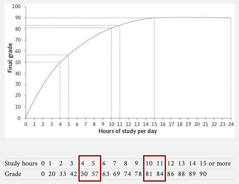
10
Diminishing Marginal Product

▪ The student’s marginal product is the increase in her grade (output)
 from increasing her study time (input) by one hour.

▪ Notice that the increase
 in final grade from
 studying 4 hours to
 studying 5 hours is 7,
 while the increase in final
 grade from studying 10
 hours to studying 11
 hours is only 3.
▪ The additional benefit of
 studying one more hour
 has diminished!

▪ A production function with this shape is described as concave.

11
Marginal Product and Average Product

▪ The marginal product is the slope of the
 line tangent to the production function.
 ‒ This will be the exact slope of the
 production function at a given number
 of study hours.
 ‒ At 4 hours of study, the marginal
 product is just above 7.

▪ The average product is calculated by
 dividing total output (final grade) by a
 particular input (number of study hours).
 ‒ This gives the average number of
 percentage points per hour of study.
 ‒ At 4 hours of study, the average
 product is 12.5 ( = 50/4 ).

▪ A diminishing marginal product implies that the average product is also diminishing.

12
So how many hours will the student study for?

▪ On its own, a production function cannot tell us what decision
 the student will make.
▪ The decision depends on the student’s preferences.
▪ If she only cared about grades, she should study for 15 hours a
 day. But the student also cares about her free time…
▪ So she faces a trade-off: how many percentage points is she
 willing to give up in order to have more free time to do things
 other than study?
▪ We now introduce the second building block of the model, which
 is called an indifference curve.

13
Building an Indifference Curve

▪ An indifference curve is a curve that connects the combinations of goods that
 provide an individual with equal levels of utility or “satisfaction.”
▪ In this case, the student
 wants a combination of a
 final grade and free time.
▪ We assume that, for a
 given grade, she prefers a
 combination with more
 free time.
▪ Similarly, for a given
 amount of free time, she
 prefers a combination with
 a higher grade.
▪ The student is indifferent
 between points along the
 same indifference curve.

14
Properties of Indifference Curves

▪ Indifference curves slope downward due to trade-offs.
 ‒ If you are indifferent between two combinations, the combination that
 has more of one good must have less of the other good.
▪ Higher indifference curves correspond to higher utility levels.
 ‒ As we move up and to the right in the diagram, further away from the
 origin, we move to combinations with more of both goods.
▪ Indifference curves are usually smooth.
 ‒ Small changes in the amounts of goods don’t cause big jumps in utility.
▪ Indifference curves do not cross.
 ‒ Why? See Exercise 3.3.
▪ As you move to the right along an indifference curve, it becomes flatter.
 ‒ Let’s investigate this last property some more…

15
The Marginal Rate of Substitution (MRS)

▪ The slope of the indifference curve is called the Marginal Rate of Substitution
 (MRS). The MRS measures the trade-off that a person is willing to make between
 two goods, at a given point on the indifference curve.
▪ The MRS changes as we move along the curve:

▪ At A, the student has an 84% grade,
 and 15 hours of free time. To gain one
 more hour of free time, the student is
 willing to sacrifice 9 percentage points,
 taking her to E.
▪ At H, the student has a 54% grade, and
 19 hours of free time. To gain one
 more hour of free time, the student is
 only willing to sacrifice 4 percentage
 points, taking her to D.

▪ So, when the student has more free time and a lower grade, the MRS is lower than
 when she has less free time and a higher grade.

16
The student’s dilemma…

▪ We can see that there is an opportunity cost associated with having more free
 time (and with having a higher grade).
 ‒ More free time means a lower grade and a higher grade means less free
 time.
 ‒ But the student wants both a high grade and a lot of free time!
▪ So how does the student pick the best combination of final grade and free
 time that she can get – the one that most satisfies the student by giving her
 the highest possible utility?
▪ To answer this question, we need the third and final building block of the
 model: the feasible frontier.

17
The Feasible Frontier

▪ The feasible frontier is the curve made of points that give the maximum feasible
 (possible) final grade that the student can achieve, given how many hours of free
 time she has.
 the slope of the frontier
 represents the opportunity
 cost of free time

▪ This is the mirror image of the production function we used earlier to determine
 the maximum possible grade the student could get, given the number of hours for
 which she studied.

18
The Feasible Set

▪ The feasible set is the area under the feasible frontier that shows all of the
 feasible combinations of free time and final grade.

▪ Any combination of free time and final grade that is on or inside the frontier is
 feasible. Combinations outside the feasible frontier are said to be infeasible given
 the student’s and conditions of study.

19
Putting the Feasible Frontier and Indifference Curves together

▪ Now that we have indifferences curves and a feasible frontier that are on the
 same axes (free time and final grade), we can put the two curves together

 We can then find a point where the trade-off the student is willing to make
 (according to the slope of her indifference curve) matches with a trade-off the
 student has to make (according to the slope of her feasible frontier).

▪ Remember that the slope of the indifference curve is called the Marginal Rate
 of Substitution (MRS).
▪ The slope of the feasible frontier also has another name: The Marginal Rate of
 Transformation (MRT).
 ‒ The MRT measures the quantity of one good that must be sacrificed to
 acquire one additional unit of another good.
 ‒ In this case, it is the rate at which the student can transform (or convert)
 free time into final grade points.

20
The MRS and the MRT

▪ The MRS is the slope of the indifference curve. It measures the trade-off that the
 student is willing to make between final grade and free time.
▪ The MRT is the slope of the feasible frontier. It measure the trade-off that the
 student is constrained to make between free time and percentage points because
 it is not possible to go beyond the feasible frontier.

▪ The student achieves the
 highest possible utility where
 the two trade-offs just balance.

▪ Her optimal combination of
 grade and free time is at the
 point where the MRT = MRS.

▪ At this point, the indifference
 curve and the feasible frontier
 are tangential to each other.

Hours of Work and Economic Growth
Technological Change

22
Another Constrained Choice Problem

▪ So far, we have considered how a student decides between studying and free
 time. This is called a constrained choice problem because the student had to
 make a choice between free time and a final grade, given her constrained
 (limited) time and productive capacity.
▪ We now apply our model to a self-sufficient farmer who chooses how many
 hours to work.
▪ We assume that the farmer produces grain to eat and does not sell it to
 anyone else. This is the only food the farmer has, so if he does not produce
 enough grain, he will starve.
▪ Like the student, the farmer also values free time. That is, he gets utility from
 both free time and consuming grain.
▪ There is an opportunity cost associated with both goods: having more free
 time means producing less grain, and producing more grain takes hours of
 labour that could otherwise be spent on free time.

23
The Farmer’s Production Function

 Remember that the slope
 of the production function
 is called the marginal
 product of labour (MPL).

▪ This is the farmer’s initial production function which shows us that he can produce 64
 units of grain if he works for 12 hours a day (point B).
▪ But what happens to this function if there is a technological improvement such as the
 invention of better farming equipment or seeds with a higher yield?

24
Technological Change and the Production Function

 Notice that PFnew is steeper
 than the PF for every given
 number of study hours. The
 new technology has increased
 the farmer’s MPL.

 This means that, at every
 point, an additional hour of
 work produces more grain
 than under the old
 technology.

▪ An improvement in technology means that more grain is produced for a given number
 of working hours. The production function shifts upward, from PF to PFnew.
▪ Now if the farmer works 12 hours per day, she can produce 74 units of grain (point C).
▪ Alternatively, by working 8 hours a day she can produce 64 units of grain (point D),
 which previously took 12 hours.

25
Technological Change and the Feasible Frontier

 Notice that FFnew is steeper
 than the FF for every given
 number of hours of free time.
 The new technology has
 increased the farmer’s MRT.

 This means that, at every
 point, an additional hour of
 free time has a higher
 opportunity cost than under
 the old technology.

▪ Technological progress expands the feasible set: it gives the farmer a wider choice of
 combinations of grain and free time.
▪ The feasible frontier shifts upward, from FF to FFnew.

26
Optimal Choice before and after Technological Change

 The farmer can move
 from point A on IC3 to
 point E on IC4, a higher
 indifference curve.

 But this is only one out
 of many possible
 movements!

▪ Technological progress raises the farmer’s standard of living: it enables him to achieve
 a higher utility than was previously possible.
▪ Note that, although the change definitely makes it feasible to both consume more
 grain and have more free time, whether the farmer will choose to have more of both
 depends on his preferences, and his willingness to substitute one good for the other.

27
Preferences are subjective

▪ We have seen that technological change has a number of effects on the
 farmer’s decision problem.
 ‒ It makes the production function steeper which increases the farmer’s
 marginal product of labour and makes the opportunity cost of free time
 higher.
 • This could give the farmer a greater incentive to work, so he may decide
 to work more and have less free time.
 • However, this change also means that the farmer can produce more
 grain in the same amount of time than he could before, so he may
 rather want to work less and have more free time.
▪ These two effects of technological progress work in opposite directions.

▪ In the next section, we look more carefully at these two opposing effects,
 using a different example to disentangle them.

Income and Substitution Effects
Budget Constraints in Constrained Choice
Problems

29
Making choices on a budget

▪ So far, we have used production functions to model the constraints that a
 student and a farmer face when making decisions on how to spend their time.
▪ Productive capacity and time are only two of many possible constraints that
 we can use in economics to investigate how people make decisions.
▪ Another constraint is money (or income) that determines how much we can
 buy or consume every day (our budget).
▪ Now we will look at how a wage earner decides how many hours to work and
 how much of their income to spend each day, based on their hourly wage.

30
The Budget Constraint

▪ In this problem, the wage earner wants both to have free time and to earn enough
 money to pay for their daily consumption (food, accommodation, entertainment
 and so on).
▪ If we let = consumption, = hourly wage, and = hours of free time per day,
 we can write the wage earner’s maximum level of consumption each day as:

 = ( − )

▪ This is the wage earner’s budget constraint. It shows what they can afford to buy.

 budget constraint
 An equation that represents all combinations of goods and services that one could
 acquire that exactly exhaust one’s budgetary resources.
 ‒ https://core-econ.org/the-economy/book/text/50-02-glossary.html#glossary

31
Drawing the budget constraint

▪ If the wage earner finds a job that pays R150 an hour (so = 150) and they need to
 spend a minimum of 8 hours taking care of themselves (sleeping, eating and so on),
 their budget constraint will look like this:
 The slope of the budget
 = ( − ) constraint corresponds to
 the wage: for each
 additional hour of free
 time (t), consumption
 must decrease by R150.

 The area under the
 budget constraint is your
 feasible set (just like the
 farmer’s feasible set).

 So, the budget constraint
 here is just like the
 BC1 farmer’s feasible frontier!

32
The Optimal Choice

▪ Remember that the slope of the feasible frontier is called the marginal rate of
 transformation (MRT), and that it represents the opportunity cost of an hour of free
 time.
▪ The feasible frontier in this case is a straight line because the rate at which the wage
 earner can transform free time into consumption is equal to the magnitude of their
 hourly wage (R150) which is constant.
 The wage earner’s preferred
 combination of consumption
 and free time will be where
 their indifference curve is
 tangential to their budget
 constraint:

 MRS = MRT = w
 At this point, their MRS —
 the rate at which they are
 willing to swap consumption
 BC1 for time — is equal to the
 wage.

33
Changes to the budget constraint: A Parallel Shift

▪ The budget constraint can shift out (or in) if there is a lump-sum increase (or decrease)
 in income.
▪ For example, if the wage earner receives R500 as a birthday gift, their budget
 constraint for that day will become BC2:

 For each amount of free
 = − + time, total income
 (earnings plus the
 birthday gift) is R500
 higher than before. So
 the budget constraint is
 shifted upwards by R500
 — the feasible set has
 expanded.

 This means that the new
 optimal choice is at point
 B on higher indifference
 curve, IC3.

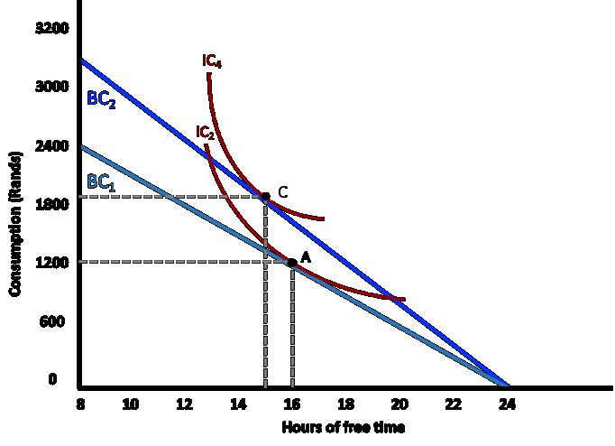
34
Changes to the budget constraint: A Swivel

▪ The budget constraint can swivel out (or in) if there is a change in the wage rate.
▪ For example, if the wage earner receives a pay rise of R45 an hour, their MRT changes
 so their budget constraint will become BC2:

 = − Now, for each hour of
 free time given up, the
 wage earner’s
 consumption can rise by
 R195 rather than R150.
 So the budget constraint
 C swivels upwards along
 the y axis — the feasible
 set has expanded.

 This means that the new
 optimal choice is at point
 C on higher indifference
 curve, IC4.

35
Different preferences yield different outcomes

▪ Compare the outcomes in the two scenarios:
 ‒ With an increase in unearned income (the birthday gift), the wage earner decides work
 fewer hours, while the wage rise leads them to increase their working hours.
 ‒ These are only examples of outcomes in each scenario; an individual’s subjective
 preferences determine the final outcome.
 ‒ We can break down the change in the optimal choice after a wage rise into two effects…

 Birthday Gift → Shift Wage Rise → Swivel
 Work fewer hours Work more hours

36
The Income and Substitution Effects

▪ A wage rise does two things:
1. It raises the income for each level of free time, expanding the feasible set and
 increasing the level of utility that can be achieved.
2. It increases the opportunity cost of free time and makes the budget constraint
 steeper.

▪ So a wage rise has two THEORETICAL effects on the choice of free time:
1. The income effect (because the budget constraint shifts outwards): the effect that the
 additional income would have if there were no change in the opportunity cost.
2. The substitution effect (because the slope of the budget constraint, the MRT, rises):
 the effect of the change in the opportunity cost, given the new level of utility.

▪ Note that The EMPIRICAL RESULT of a wage rise depends on whether the income effect
 or substitution effect is larger:
 - If income effect > substitution effect – free time increases
 - If income effect < substitution effect – free time falls

37
The Income Effect in this case, explained

income effect
The effect that the additional income would have if there were no change in the price or
opportunity cost.

▪ A wage rise means that the wage earner can get more income for every one hour
 worked.
▪ As a result, they more willing to sacrifice consumption for extra free time, since they
 can consume more for a given amount of free time.
▪ This happens because their feasible set has expanded.
▪ The wage earner responds to additional income by taking more free time as well as
 increasing consumption. This is called the income effect.

▪ We assume that for most goods the income effect will be either positive or zero, but
 not negative: if income increases, an individual would not choose to have less of
 something that they valued.

38
The Substitution Effect in this case, explained

substitution effect
The effect that is only due to changes in the price or opportunity cost, given the new level
of utility.

▪ A wage rise means that the wage earner loses more income for every one hour NOT
 worked.
▪ As a result, they are less willing to sacrifice consumption for extra free time, since the
 opportunity cost of free time is higher.
▪ This happens because their marginal rate of transformation (MRT) is higher.
▪ The wage earner responds to increases in the opportunity cost of free time by taking
 less free time. This is called the substitution effect.

▪ The substitution effect captures the idea that, when a good becomes more expensive
 relative to another good, you choose to substitute some of the other good for it.

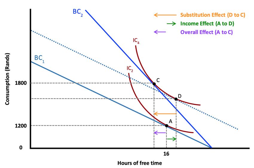
39
The Income and Substitution Effects on the diagram

▪ The overall effect of the wage rise depends on the sum of the income and substitution
 effects. In this case, the substitution effect is bigger, so with the higher wage you take less
 free time.

Is this realistic?
Do people think about MRS and MRT every day?

41
Economic theory helps to explain what people do

▪ Billions of people organize their working lives without knowing anything about MRS
 and MRT. So how can this model be useful?
▪ Remember from Unit 2 that models help us ‘see more by looking at less’. Lack of
 realism is an intentional feature of this model, not a shortcoming.
▪ Economists do not actually claim that people actually think through these calculations
 (such as equating MRS to MRT) each time we make a decision.

▪ Trial and error replaces calculations
 ‒ Different people each try various choices (sometimes not even intentionally) and
 tend to adopt habits, or rules of thumb that make them feel satisfied and avoid
 regret. Eventually we could speculate that they might end up with a decision on
 work time that is close to the result of our calculations.
▪ The influence of culture and politics
 ‒ Although individual workers often have little freedom to choose their hours, it may
 nevertheless be the case that changes in working hours over time, and differences
 between countries, partly reflect the preferences of workers.

Worldwide Working Hours
How do countries decide how much to work?

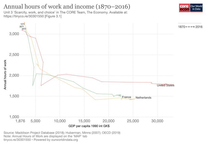
43
Working hours have changed over time…

▪ From the late nineteenth century (1800s) until the middle of the twentieth century
 (1900s), working time in many countries gradually fell…

44
Why?

▪ The simple models we have constructed cannot tell the whole story. Remember that
 the ceteris paribus assumption can omit important details: things that we have held
 constant in models may vary in real life.
▪ Our model omitted two important explanations, which we called culture and politics.
 Our model provides another explanation: economics.

▪ We can use the model and the concepts we’ve learned so far to explain historical
 change.

45
South Africa’s Basic Conditions of Employment Act 75 of 1997

▪ Your employer is not allowed to require
 or permit you to work more than:
 ‒ 45 hours a week.
 ‒ Nine hours in a day if you work on 5
 days or less a week.
 ‒ Eight hours in a day if you work more
 than 5 days a week.
 ‒ You must have a meal interval of 60
 minutes after five hours of work. This
 may be reduced to 30 minutes by
 written agreement.
 ‒ Your lunch break may also be done
 away with by written agreement if
 you work less than 6 hours a day.

46
Possible feasible sets and indifference curves

▪ We can interpret the change between 1900 and 2013 in daily free time and goods per
 day for employees in the US using our model. The solid lines show the feasible sets for
 free time and goods in 1900 and 2013, where the slope of each budget constraint is
 the real wage.
▪ Assuming that workers chose the hours they worked, we can infer the approximate
 shape of their indifference curves:

47
The Income Effect over the 20th century in the US

▪ Before 1900, low consumption levels meant that workers’ willingness to substitute free time
 for goods did not increase much when rising wages made higher consumption possible. But
 by the 1900s, workers had a higher level of consumption and valued free time relatively
 more — their marginal rate of substitution was higher — so the income effect of a wage rise
 was larger than before.
▪ The shift from A to C is the income effect of the wage rise, which on its own would cause US
 workers to take more free time.

48
The Substitution Effect over the 20th century in the US

▪ At the same time, workers were more productive and were paid more, so each hour of work
 brought more rewards than before in the form of consumption, increasing the incentive to
 work longer hours.
▪ The rise in the opportunity cost of free time caused US workers to choose D rather than C,
 with less free time.

49
The Overall Effect over the 20th century in the US

▪ The overall effect of the wage rise depends on the sum of the income and substitution
 effects:
 ‒ Before 1900, the negative substitution effect (free time falls) was bigger than the positive
 income effect (free time rises), so work hours rose.
 ‒ In the 1900s, the income effect began to outweigh the substitution effect, working time
 fell.

50
Preferences can also change over time

▪ Over time, people change their preferences and can value consumption more or less
 than they did before, because of personal, cultural, political and economic changes.
▪ Popular culture, fashion and trends such as trying to “keep up with the Joneses” can
 also influence people’s spending behaviour.
 conspicuous consumption
 The purchase of goods or services to publicly display one’s social and economic status.
 ‒ https://core-econ.org/the-economy/book/text/50-02-glossary.html#glossary

▪ People’s preferences will continue to change in future and different economies will
 change in different ways…

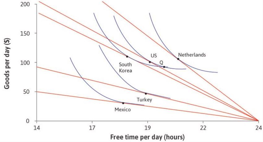
51
Comparing countries

▪ We can use our model to understand the differences between the countries. The solid lines
 show the feasible sets of free time and goods for the five countries.
▪ Notice that the indifference curves for the US and for South Korea cross. This means that
 South Koreans and Americans must have different preferences.
▪ Point Q is at the intersection of the indifference curves for the US and South Korea. At this
 point Americans are willing to give up more units of daily goods for an hour of free time
 than South Koreans.

52

https://www.youtube.com/watch?v=91TgP1D0Kps&t=317s

Conclusion

54
Main points again

▪ People’s preferences with respect to goods and free time are described by indifference
 curves.
▪ Their production function (or budget constraint) determines their feasible set.
▪ The choice that maximizes utility is a point on the feasible frontier where the marginal
 rate of substitution (MRS) between goods and free time is equal to the marginal rate
 of transformation (MRT).

▪ An increase in productivity or wages alters the MRT, raising the opportunity cost of
 free time. This provides an incentive to work longer hours (the substitution effect). But
 higher income may increase the desire for free time (the income effect).
▪ The overall change in hours of work depends on which of these effects is bigger.