Semantic representation of Slovak words - CEUR Workshop ...
←
→
Page content transcription
If your browser does not render page correctly, please read the page content below
Semantic representation of Slovak words

                                        Šimon Horvát1 , Stanislav Krajči, and L’ubomír Antoni

                            Institute of Computer Science, Pavol Jozef Šafárik University in Košice, Slovakia,
                                                       simon.horvat@upjs.sk,

Abstract: The first problem one encounters when trying                    with mentioned properties, we apply well-known feature
to apply analytical methods to text data is probably that                 learning algorithm Node2Vec for networks. This method
of how to represent it in a way that is amenable to opera-                interprets nodes as vectors that are suitable for use as word
tions such as similarity, composition, etc. Recent methods                vectors with semantic properties.
for learning vector space representations of words have                      We focus on the process of Slovak words to increase
succeeded in capturing semantic using vector arithmetic,                  the automated processing (NLP) of Slovak language, but
however, all of these methods need a lot of text data for                 it can be used for any other language. The paper is orga-
representation learning.                                                  nized as follows: Section 2 – Related works, we present
   In this paper, we focus on Slovak words representation                 the basic definitions, and briefly describes methods from
that captures semantic information, but as the data source,               related works. Section 3 – Data processing, explores our
we use a dictionary, since the public corpus of the required              data sources and their processing for the usage of our
size is not available. The main idea is to represent infor-               method. In Section 4 – Methods, We propose a novel
mation from the dictionary as a word network and learn a                  approach, which produces dense vector representations of
mapping of nodes to a low-dimensional space of features                   words with semantic properties. Some results are shown
that maximize the likelihood of preserving network neigh-                 in section 5 – Experiments, and key takeaway ideas are
bourhoods of word nodes.                                                  discussed in the last section 6 – Conclusion.

1    Introduction                                                         2   Related works

Recently, the area of natural language processing (NLP)                   Semantic vector space models of language represent each
passed reform. Even this area did not escape the strong                   word with a real-valued vector. These representations are
influence of the rise of neural networks. In most NLP clas-               now commonly called word embeddings. The vectors can
sical tasks, such as text classification, machine translation,            be used as features in a variety of applications as stated in
sentiment analysis, good results are achieved because of                  the previous chapter. Distance between every two vectors
deep learning-based representation of fundamental build-                  should reflect how closely relate the meaning of the words,
ing language components – words. Neural networks use                      in ideal semantic vector space. The goal is to achieve an
large corpora for word representation learning [5][6].                    approximation of this vector space.
   However, in some languages, it is not possible to use                     Word embeddings are commonly ([8][9][10]) catego-
this approach because it does not exist large amounts of                  rized into two types, depending upon the strategies used
unstructured text data in them. These issues can be well                  to induce them. Methods that leverage local data (e.g. a
illustrated by Google translations in some not widely spo-                word’s context) are called prediction-based models and are
ken languages (see Figure 1). The reason for poor transla-                generally reminiscent of neural language models. On the
tions is the absence of a large public source of text data.               other hand, methods that use global information, generally
   In this paper, we propose our approach, which aims to                  corpus-wide statistics such as word counts and frequencies
obtain the semantic representation of words based on pub-                 are called count-based models [4].
lic dictionaries instead of the corpus. The main idea is                     Both types of models have their advantages and disad-
to construct graph G = (V, E, φ ) where vertices are words,               vantages. However, a significant drawback of both ap-
which we want to get vector representation from and edges                 proaches for not widely spoken language is the need for
are relationships between words. It means the words that                  a large corpus. In the following sections, we show how
are closely related will be connected by an edge. The in-                 can be this problem solved.
tensity of this relationship is expressed by weight – the
real number from 0 to 1. As our source of data for build-                 Prediction-based models. The idea of this approach is to
ing graph G, we used dictionaries. We will describe details               learn word representations that aid in making predictions
in the section Data processing. We use tf-idf statistics                  within local context windows (Figure 2). For example,
for weighting our word network. After building graph G                    Mikolov et al. [5] have introduced two models for learn-
      Copyright c 2020 for this paper by its authors. Use permitted un-
                                                                          ing embeddings, namely the continuous bag-of-words
der Creative Commons License Attribution 4.0 International (CC BY         (CBOW) and skip-gram (SG) models (Figure 3). The
4.0).                                                                     main difference between CBOW and SG lies in the loss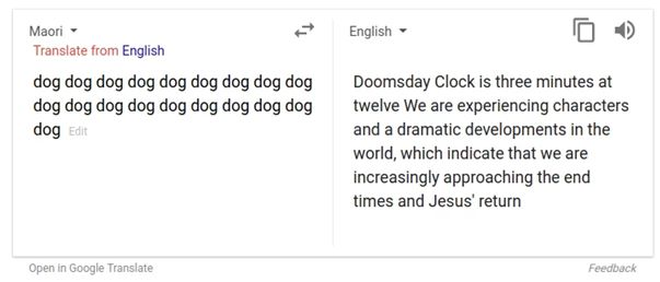
Figure 1: The languages that generate the strangest results – Somali, Hawaiian and Maori – have smaller bodies of
translated text than more widely spoken languages like English or Chinese. As a result, it’s possible that Google used
religious texts like the Bible, which has been translated into many languages [20].

Figure 2: Local context windows. This figure shows some of the training samples (word pairs) we would take from the
sentence "The quick brown fox jumps over the lazy dog." It used a small window size of 2 just for the example. The word
highlighted in blue is the center word. The creation of a dataset for a neural network consists in such processing of each
sentence in the corpus [19].

function used to update the model, while CBOW trains           3     Data processing
a model that aims to predict the center word based upon
its context, in SG the roles are reversed, and the center      As we already mentioned, we use dictionaries as our data
word is, instead, used to predict each word appearing in       source instead of corpora. First at all, we find web page,
its context.                                                   which contains dictionaries with public access for pulling
                                                               data out of HTML (it is also possible to use dictionaries in
Count-based models. These models are another way               text format). We parse two types of Dictionary:
of producing word embeddings, not by training algo-                1. Synonym dictionary [14],
rithms that predict the next word given its context but by
leveraging word-context cooccurence counts globally in             2. classic dictionary [13] that contains a list of words
a corpus. These are very often represented (Turney and                and their meaning.
Pantel (2010) [15]) as word-context matrices. The earliest        First, we establish some notation. Let VOCAB be a set
relevant example of leveraging word-context matrices to        of all words that we want to represent as a vector.
produce word embeddings is Latent Semantic Analysis               Let S represent the set of all synonym pairs achieved
(LSA) (Deerwester et al. (1990) [11]) where Singular           from the Synonym dictionary [14]. Set S contains pairs
value decomposition (SVD) is applied [4].                      like
                                                                (vtipný, zábavný), (vtipný, smiešny), (rýchlo, chytro) . . .
Figure 3: Skip-gram network architecture (the coded vocabulary is illustrative). As input, skip-gram expects center
word in one-hot representation. The layer in the middle has the number of neurons as the desired dimension of word
embeddings. The last layer tries to predict the probability distribution of the occurrence of words in the context of the
center word. Metrix of weights between the middle and the last layer is word vectors [19].

It is important to remark that not every word from                         4.1   tf-idf
VOCAB has synonym pair. Let L represent the set of
word pairs from the Dictionary [13].                                       The notion tf-idf stands for term frequency-inverse doc-
   We create these word pairs (w, li ) as follow:                          ument frequency, and the tf-idf weight is a weight often
    • For word w from VOCAB, we find its definition from                   used in information retrieval and text mining. This weight
      the Dictionary [13].                                                 is a statistical measure used to evaluate how important a
                                                                           word is to a document in a collection or corpus. The im-
    • Subsequently, we find the lemma of each word oc-                     portance increases proportionally to the number of times
      curring in this definition of w. Let denote these lem-               a word appears in the document but is offset by the fre-
      mas as l1 , l2 , . . . , ln . For each word w from VOCAB,            quency of the word in the corpus. Variations of the tf-idf
      there are pairs (w, l1 ), (w, l2 ), . . . , (w, ln ) in set L. For   weighting scheme are often used by search engines as a
      instance, word slnko has definition: “Nebeské teleso                 central tool in scoring and ranking a document’s relevance
      vysielajúce do vesmíru teplo a svetlo.” Based on that,               given a user query. The tf-idf can be successfully used
      we add to set L these pairs: (slnko, nebeský), (slnko,               for stop-words filtering in various subject fields, including
      teleso), (slnko, vysielajúce), (slnko, vesmír), (slnko,              text summarization and classification. The tf-idf is the
      teplo), (slnko, svetlo).                                             product of two statistics, term frequency and inverse doc-
We used a rule-based tool for lemitization [16][17][18].                   ument frequency [2][3].
   Let G = (V, E, φ ) to be denoted by a directed graph
where V = VOCAB, edges E = S ∪ L and φ is the func-                        Term frequency. Suppose we have a set of English text
tion that for each edge e from E assign real number φ (e).                 documents and wish to rank which document is most rel-
We will define function φ in section 4.1.                                  evant to the query, "the brown cow". A simple way to
   From now, our initial task of word representation learn-                start out is by eliminating documents that do not contain
ing is transformed into a graph-mining problem.                            all three words "the", "brown", and "cow", but this still
                                                                           leaves many documents. To further distinguish them, we
4     Methods                                                              might count the number of times each term occurs in each
                                                                           document; the number of times a term occurs in a docu-
In this section, we present the tf-idf method and                          ment is called its term frequency. In the case of the term
Node2Vec algorithm [1].                                                    frequency tf(t, d), the simplest choice is to use the raw
Figure 4: Node2Vec embedding process [21]
count of a term in a document, i.e., the number of times tf-idf as a weight function. Let’s consider word železný
that term t occurs in document d. and its definition “obsahujúci železo; majúci istý vzt’ah
k železu”. For Slovak readers, it is obvious not every
Inverse document frequency. Because the term "the" is so word of the definition is related to the word železný in the
common, term frequency will tend to incorrectly empha- same way. Some words are very important for the con-
size documents that happen to use the word "the" more struction of definition (obsahujúci, mat’, istý) but they are
frequently, without giving enough weight to the more not related to the defined word. By the definition of our
meaningful terms "brown" and "cow". The term "the" word network G, all lemmas will be joined with the word
is not a good keyword to distinguish relevant and non- železný by an edge, but we can filter unrelated words by
relevant documents and terms, unlike the less-common assigning them low weight.
words "brown" and "cow". Hence an inverse document
frequency factor is incorporated which diminishes the • tf(t, d) the number of times that word t occurs in
weight of terms that occur very frequently in the document definition d. For instance, tf(železo, “obsahujúci
set and increases the weight of terms that occur rarely. So železo; mat’ istý vzt’ah železo”) = 2.
the inverse document frequency is a measure of how much
• idf(t, D) is inverse document frequency defined as
information the word provides, i.e., if it’s common or rare
(1), where D is set of all definitions from the Dictio-
across all documents. It is the logarithmically scaled in-
nary,
verse fraction of the documents that contain the word (ob-
tained by dividing the total number of documents by the – N is total number of definitions,
number of documents containing the term, and then taking – and |{d ∈ D : t ∈ d}| is number of definitions
the logarithm of that quotient): where the word t appears.
N
idf(t, D) = log (1) The definition implies that often appearing words in def-
|{d ∈ D : t ∈ d}| initions (such as "majúci" or "nejaký") have a low idf
with value. So the relationship between words w and li (lemma
• N: total number of documents in the corpus N = |D| of i-th word that appears in definition dw of word w) is
given by value tf-idf(w, li ) = tf(li , dw ) · idf(li , D).
• |{d ∈ D : t ∈ d}| number of documents where the term tf-idf is our weight function if edge e join word w1
t appears. and word w2 , where w2 is the lemma of a word that appears
in definition dw1 of word w, in other words, if e from L. If
Term frequency–Inverse document frequency. tf-idf is edge e join synonyms words (e ∈ S), the weight of e is 1 –
calculated as a max weight value. If e belongs L but also e belongs S,
tf-idf(t, d, D) = tf(t, d) · idf(t, D) φ (e) = 1.
A high weight in tf-idf is reached by a high term fre-
quency (in the given document) and a low document fre- 1,
if e ∈ S
quency of the term in the whole collection of documents; φ (e) = φ (w1 , w2 ) = tf-idf(w1 , w2 ), if e ∈ L
the weights hence tend to filter out common terms. Since
1, if e ∈ S ∩ L
the ratio inside the idf’s log function is always greater
than or equal to 1, the value of idf (and tf-idf) is greater
4.2 Node2Vec
than or equal to 0. As a term appears in more documents,
the ratio inside the logarithm approaches 1, bringing the In previous sections, we have described building graph
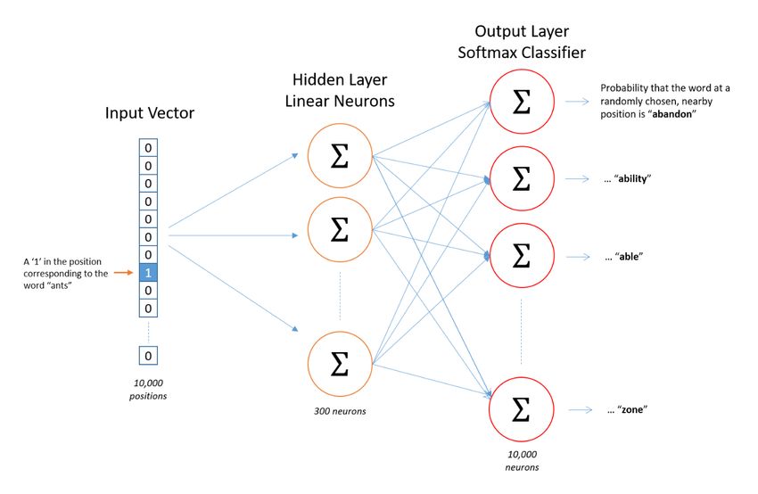
idf and tf-idf closer to 0. G = (V, E, φ ) that captures the semantic relationships be-Figure 5: Node2Vec embedding process [1]
tween words. Finally, we need to obtain a vector repre- encourages moderate exploration and avoids 2-hop redun-
sentation of each node of a graph. We use the Node2Vec dancy in sampling. On the other hand, if p is low, it would
algorithm for this purpose [1]. The Node2Vec frame- lead the walk to backtrack a step and this would keep the
work learns low-dimensional representations for nodes in walk "local" close to the starting node u.
a graph through the use of random walks. Given any In-out parameter q allows the search to differentiate be-
graph, it can learn continuous feature representations for tween "inward" and "outward" nodes. Going back to Fig-
the nodes, which can then be used for various downstream ure 5, if q > 1, the random walk is biased towards nodes
machine learning tasks. Node2Vec follows the intuition close to node t. Such walks obtain a local view of the un-
that random walks through a graph can be treated like derlying graph with respect to the start node in the walk
sentences in a corpus (sampling strategy). Each node in and approximate BFS (Breadth First Search Traversal) be-
a graph is treated like an individual word, and a random havior in the sense that our samples comprise of nodes
walk is treated as a sentence. When we have a sufficiently within a small locality. In contrast, if q < 1, the walk is
large corpus obtained by random walks through the graph, more inclined to visit nodes that are further away from the
the next step of the algorithm is to use the traditional em- node t. Such behavior is reflective of DFS (Deph First
bedding technique to obtain vector representation (see Fig- Search Traversal) which encourages outward exploration.
ure 4), in the concrete, Node2Vec use mentioned skip- However, an essential difference here is that we achieve
gram model (Figure 3). Node2Vec algorithm works in 2 DFS-like exploration within the random walk framework.
steps: sampling strategy and feeding the skip-gram model. Hence, the sampled nodes are not at strictly increasing dis-
Since we already mention skip-gram model, we will focus tances from a given source node u, but in turn, we benefit
on the sampling strategy. from tractable preprocessing and superior sampling effi-
Node2Vec’s sampling strategy, accepts four arguments: ciency of random walks [1].
For weighted graphs (our case), the weight of the edge
• Number of walks n: Number of random walks to be has an impact on the probability of node visiting (higher
generated from each node in the graph, weight - the higher probability of visiting).
• walk length l: how many nodes are in each random
walk,
5 Experiments
• p: return hyperparameter,
The word similarity measure is one of the most frequently
• q: in-out hyperparameter. used approaches to validate word vector representations.
The word similarity evaluator correlates the distance be-
The first two hyperparameters are self-explanatory. The tween word vectors and human perceived semantic simi-
algorithm for the random walk generation will go over larity. The goal is to measure how well the notion of hu-
each node in the graph and will generate n random walks, man perceived similarity is captured by the word vector
of length l. representations.
Return parameter p controls the likelihood of immedi-
One commonly used evaluator is the cosine similarity
ately revisiting a node in the walk. Setting it to a high
defined by
value ensures that we are less likely to sample an already
visited node in the following two steps (unless the next wx · wy
node in the walk had no other neighbor). This strategy cos(wx , wy ) = ,
kwx k · kwy kFigure 6: Word meanings communities of kobylka in word vector space.
where wx and wy are two word vectors and kwx k and kwy k Figure 6 shows that our word vector space captures the
are the L2 norm. individual meanings of words by grouping words from one
This test computes the correlation between all vector di- meaning into the community.
mensions, independent of their relevance for a given word
pair or a semantic cluster. Many datasets are created for
word similarity evaluation, unfortunately, there is no this 6 Conclusion
kind of dataset for the Slovak language. In Table 1, we
present the several words and list of their 20 nearest words, In this work, we offer a solution to the problem of a lack of
which are the results of our proposed model. We use co- text data for building word embedding. As a data source,
sine similarity as our distance metric and following setting we use a dictionary instead of a corpus. From the data, we
of Node2Vec algorithm: have constructed the word network in which we transform
each node into the vector space. In the section Experi-
• Number of walks n: 20, ments, we show that word vectors capture semantic infor-
mation what is the main idea behind of word embedding.
• walk length l: 100, In addition, we have presented that vector space captures
more senses for multiple meaning words.
• p: 10, As a possible extension of this work is to enrich our
• q: 1. vector space with grammatical information too (vectors of
adjectives will be closer to each other than vectors of ad-
Several words in Table 1 have multiple meaning. For jective and verb). As we already mentioned, our graph
example, kobylka has 3 meanings: contains only word lemmas, but it is also possible to add
different shapes of a word into vector space.
1. miniature of a mare, female horse, In addition, we have presented that vector space is an
appropriate representation for multiple meaning words.
2. meadow jumping insect,
3. a string-supporting component of musical instru-
ments.radost’ korenie srdce film huba tanec ticho kobylka učit’ rýchlo modra verný
lala oregano dušička celuloidový špongia kozáčik nehlučne kobyla vštepovat’ šmihom modrunký nepredstieraný
zal’úbenie bobul’ka dušinka pornofilm trúdnik tarantela nehlasne sláčikový zaúčat’ friško svetlobelasý doslovný
jasot čili drahá kinosála michalka sarabanda bezhrmotne saranča vzdelávat’ expresne blankytný úprimne
úl’uba fenikel zlatko diafilm smrčok špásy nezvučne lúčny zaškol’ovat’ zvrtkom temnobelasý skalný
slast’ maggi milá krimi tlama tancovačka bezhlasne šalvia školit’ prirýchlo namodravý mravčí
radostiplný škorica červeň filmotéka hl’uzovka odzemok neslyšne šidlo školovat’ gvaltom kobaltový faktický
potešenie okorenit’ srdiečko kinofilm papul’a foxtrot tlmene toccata navykat’ nanáhlo nezábudkový vytrvalý
potecha korenička chrobáčik vel’kofilm čírovka rumba potíšku koník cvičit’ chvátavo slabomodrý pravdivý
pôžitok d’umbier miláčik mikrofiš mykológia kratochvíl’a tíš stradivárky muštrovat’ chvatom temnomodrý predstieraná
optimizmus korenina holúbok indiánka hubárčit’ menuet bezhlučne škripky privykat’ nanáhle jasnobelasý ozajstný
rozkoš vanilka st’ah vývojka hubárka kankán tlmeno prím priúčat’ chytro bledobelasý faksimile
blaženost’ pokorenit’ srdcovitý porno bedl’a radovánky bezzvučne tepovač zvykat’ prichytro nebovomodrý neprestávajúci
ujujú majorán srdciar nitrocelulóza hubár mazúrka neslyšatel’ne mučidlo vyučovat’ zrýchlene azúrový opravdivý
t’jaj sušený kardiogram kovbojka peronospóra twist potíšky husl’ový memorovat’ švihom zafírovomodrý vytrvanlivý
optimista temian centrum videofilm zvonovec tamburína nečujne husle osvojovat’ skokmo zafírový naozajský
rozšt’astnený puškvorec stred predpremiéra podpňovka polonéza pridusene žrebica trénovat’ promptne ultramarínový úprimný
prešt’astlivý pamajorán trombóza premietareň múčnatka zábavka nepočutel’ne viola študírovat’ habkom nevädzový neskreslený
ujú aníz kardiograf pornohviezda plávka charleston zmĺknuto husliar hlásat’ úvalom nevädzí vtelený
zvesela zázvor drahý detektívka dubák tango tíško struna samouk bleskurýchle tuhobelasý nefalšovaný
Table 1: The nearest 20 words to the first bold word.References [17] S. Krajči, R. Novotný – databáza tvarov slov slovenského
jazyka, Informačné technológie – Aplikácie a teória, zborník
príspevkov z pracovného seminára ITAT, 17.–21. septem-
ber 2012, Monkova dolina (Slovensko), Košice, SAIS,
[1] A. Grover and J. Leskovec: node2vec – Scalable feature
Slovenská spoločnost’ pre umelú inteligenciu, 2012, ISBN
learning for networks. In Proceedings of the 22nd ACM
9788097114411, s. 57–61
SIGKDD International Conference on Knowledge Discov-
ery and Data Mining. ACM, 2016. [18] S. Krajči, R. Novotný: Projekt Tvaroslovník – slovník
všetkých tvarov všetkých slovenských slov, Znalosti 2012,
[2] J. Ramos: Using tf-idf to determine word relevance in docu-
zborník príspevkov 11. ročníka konferencie: 14. - 16. ok-
ment queries. In ICML, 2003.
tóber 2012, Mikulov (Česko), Praha, MATFYZPRESS, Vy-
[3] S. Robertson: Understanding inverse document frequency: davatelství MFF UK v Praze, 2012, ISBN 9788073782207,
On theoretical arguments for IDF. Journal of Documentation s. 109–112
[4] J. Pennington, R. Socher, and Ch. D. Manning: Glove [19] C. McCormick: Word2Vec Tutorial - The Skip-Gram
– Global vectors for word representation. In Conference Model. Retrieved from http://www.mccormickml.com,
on Empirical Methods on Natural Language Processing 2016, April 19.
(EMNLP)
[20] J. Christian: Why Is Google Translate Spitting Out Sinis-
[5] T. Mikolov, K. Chen, G. Corrado, and J. Dean: Efficient Es- ter Religious Prophecies? Retrieved from https://www.
timation of Word Representations in Vector Space. In ICLR vice.com/en_us, 2018.
Workshop Papers 2013a
[21] E. Cohen: node2vec: Embeddings for Graph Data. Re-
[6] G. Almeida, F. Xexéo: Word embeddings – a survey. arXiv trieved from https://towardsdatascience.com/, 2018.
preprint arXiv:1901.09069 (2019)
[7] T. Young, D. Hazarika, S. Poria, E. Cambria: Recent trends
in deep learning based natural language processing. IEEE
Computational Intelligence Magazine (2018).
[8] M. Baroni, G. Dinu, and G. Kruszewski: Don’t count,
predict! a systematic comparison of context-counting vs.
context-predicting semantic vectors. In Proceedings of the
52nd Annual Meeting of the Association for Computational
Linguistics (Volume 1: Long Papers). Association for Com-
putational Linguistics, June 2014.
[9] R. Socher, J. Pennington, E. H. Huang, A. Y. Ng, and Ch. D.
Manning: Semi-supervised recursive autoencoders for pre-
dicting sentiment distributions. In Proceedings of the Con-
ference on Empirical Methods in Natural Language Process-
ing, EMNLP ’11. Association for Computational Linguistics
2011.
[10] S. Li, J. Zhu, and Ch. Miao: Agenerative word embedding
model and its lowrank positive semidefinite solution 2015.
[11] S. Deerwester, S. T. Dumais, G. W. Furnas, T. K. Lan-
dauer, and R. Harshman: Indexing by latent semanticanal-
ysis, 1990.
[12] K. Bollacker, D. Kurt, C. Lee: An Autonomous Web Agent
for Automatic Retrieval and Identification of Interesting
Publications. Proceedings of the Second International Con-
ference on Autonomous Agents. AGENTS ’98. pp. 116–123.
[13] L’. Štúr Institute of Linguistics of the Slovak Academy of
Sciences (SAS): Krátky slovník slovenského jazyka 4. 2003
– kodifikačná príručka. Retrieved from https://slovnik.
aktuality.sk/
[14] L’. Štúr Institute of Linguistics of the Slovak Academy of
Sciences (SAS): Synonymický slovník slovenčiny, 2004.Re-
trieved from https://slovnik.aktuality.sk/
[15] P. D. Turney, P. Pantel: From Frequency to Meaning: Vec-
tor Space Models of Semantics. In Journal of Artificial In-
telligence Research
[16] S. Krajči, R. Novotný, L. Turlíková, M. Laclavík: The
tool Morphonary/Tvaroslovník: Using of word lemmatiza-
tion in processing of documents in Slovak, in: P. Návrat,
D. Chudá (eds.), Proceedings Znalosti 2009, Vydavatel’stvo
STU, Bratislava, 2009, s. 119-130You can also read