SEMEVAL-2020 TASK 1: UNSUPERVISED LEXICAL SEMANTIC CHANGE DETECTION
←
→
Page content transcription
If your browser does not render page correctly, please read the page content below
SemEval-2020 Task 1:
                                                              Unsupervised Lexical Semantic Change Detection
                                                        Dominik Schlechtweg,♣ Barbara McGillivray,♦,♥ Simon Hengchen,♠∗
                                                                         Haim Dubossarsky,♥ Nina Tahmasebi♠
                                                           semeval2020lexicalsemanticchange@turing.ac.uk
                                                     ♣
                                                       University of Stuttgart, ♦ The Alan Turing Institute, ♥ University of Cambridge
                                                                                 ♠
                                                                                   University of Gothenburg

                                                                                             Abstract
                                                 Lexical Semantic Change detection, i.e., the task of identifying words that change meaning
                                                 over time, is a very active research area, with applications in NLP, lexicography, and linguistics.
arXiv:2007.11464v2 [cs.CL] 28 Aug 2020

                                                 Evaluation is currently the most pressing problem in Lexical Semantic Change detection, as no
                                                 gold standards are available to the community, which hinders progress. We present the results of
                                                 the first shared task that addresses this gap by providing researchers with an evaluation framework
                                                 and manually annotated, high-quality datasets for English, German, Latin, and Swedish. 33 teams
                                                 submitted 186 systems, which were evaluated on two subtasks.

                                         1       Overview
                                         Recent years have seen an exponentially rising interest in computational Lexical Semantic Change (LSC)
                                         detection (Tahmasebi et al., 2018; Kutuzov et al., 2018). However, the field is lacking standard evaluation
                                         tasks and data. Almost all papers differ in how the evaluation is performed and what factors are considered
                                         in the evaluation. Very few are evaluated on a manually annotated diachronic corpus (McGillivray et al.,
                                         2019; Perrone et al., 2019; Schlechtweg et al., 2019, e.g.). This puts a damper on the development of
                                         computational models for LSC, and is a barrier for high-quality, comparable results that can be used in
                                         follow-up tasks.
                                            We report the results of the first SemEval shared task on Unsupervised LSC detection.1 We introduce
                                         two related subtasks for computational LSC detection, which aim to identify the change in meaning of
                                         words over time using corpus data. We provide a high-quality multilingual (English, German, Latin,
                                         Swedish) LSC gold standard relying on approximately 100,000 instances of human judgment. For the
                                         first time, it is possible to compare the variety of proposed models on relatively solid grounds and across
                                         languages, and to put previously reached conclusions on trial. We may now provide answers to questions
                                         concerning the performance of different types of semantic representations (such as token embeddings vs.
                                         type embeddings, and topic models vs. vector space models), alignment methods and change measures.
                                         We provide a thorough analysis of the submitted results uncovering trends for models and opening
                                         perspectives for further improvements. In addition to this, the CodaLab website will remain open to
                                         allow any reader to directly and easily compare their results to the participating systems. We expect the
                                         long-term impact of the task to be significant, and hope to encourage the study of LSC in more languages
                                         than are currently studied, in particular less-resourced languages.

                                         2       Subtasks
                                         For the proposed tasks we rely on the comparison of two time-specific corpora C1 and C2 . While this
                                         simplifies the LSC detection problem, it has two main advantages: (i) it reduces the number of time
                                         periods for which data has to be annotated, so we can annotate larger corpus samples and hence more
                                         reliably represent the sense distributions of target words; (ii) it reduces the task complexity, allowing
                                                 ∗
                                              SH was affiliated with the University of Helsinki and the University of Geneva for most of this work.
                                             1
                                            https://languagechange.org/semeval. In the remainder of this paper, “CodaLab” refers to this URL.
                                         This work is licensed under a Creative Commons Attribution 4.0 International License. License details: http://
                                         creativecommons.org/licenses/by/4.0/.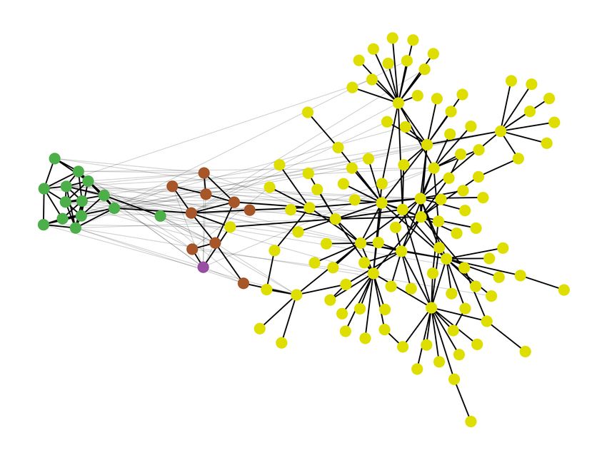
C1                          C2
                        Senses   chamber   biology   phone   chamber   biology   phone
                        # uses      12       18        0        4        11       18

            Table 1: An example of a sense frequency distribution for the word cell in C1 and C2 .

different model architectures to be applied to it, widening the range of possible participants. Participants
were asked to solve two subtasks:

 Subtask 1 Binary classification: for a set of target words, decide which words lost or gained sense(s)
    between C1 and C2 , and which ones did not.
 Subtask 2 Ranking: rank a set of target words according to their degree of LSC between C1 and C2 .

For Subtask 1, consider the example of cell in Table 1, where the sense ‘phone’ is newly acquired from
C1 to C2 because its frequency is 0 in C1 and > 0 in C2 . Subtask 2, instead, captures fine-grained
changes in the two sense frequency distributions. For example, Table 1 shows that the frequency of the
sense ‘chamber’ drops from C1 to C2 , although it is not totally lost. Such a change will increase the
degree of LSC for Subtask 2, but will not count as change in Subtask 1. The notion of LSC underlying
Subtask 1 is most relevant to historical linguistics and lexicography, while the majority of LSC detection
models are rather designed to solve Subtask 2. Hence, we expected Subtask 1 to be a challenge for most
models. Knowing whether, and to what degree a word has changed is crucial in other tasks, e.g. aiding in
understanding historical documents, searching for relevant content, or historical sentiment analysis. The
full LSC problem can be seen as a generalization of these two tasks into multiple time points where also
the type of change needs to be identified.

3       Data
The task took place in a realistic unsupervised learning scenario. Participants were provided with trial
and test data, but no training data. The public trial and test data consisted of a diachronic corpus pair
and a set of target words for each language. Participants’ predictions were evaluated against a set of
hidden gold labels. The trial data consisted of small samples from the test corpora (see below) and four
target words per language to which we assigned binary and graded gold labels randomly. Participants
could not use this data to develop their models, but only to test the data input format and the online
submission format. For development data participants were referred to three pre-existing diachronic data
sets: DURel (Schlechtweg et al., 2018), SemCor LSC (Schlechtweg and Schulte im Walde, 2020) and
WSC (Tahmasebi and Risse, 2017). In the evaluation phase participants were provided with the test
corpora and a set of target words for each language.2 Participants were asked to train their models only on
the corpora described in Table 2, though the use of pre-trained embeddings was allowed as long as they
were trained in a completely unsupervised way, i.e., not on manually annotated data.

3.1      Corpora
For English, we used the Clean Corpus of Historical American English (CCOHA) (Davies, 2012; Alatrash
et al., 2020), which spans 1810s–2000s. For German, we used the DTA corpus (Deutsches Textarchiv,
2017) and a combination of the BZ and ND corpora (Berliner Zeitung, 2018; Neues Deutschland, 2018).
DTA contains texts from different genres spanning the 16th–20th centuries. BZ and ND are newspaper
corpora jointly spanning 1945–1993. For Latin, we used the LatinISE corpus (McGillivray and Kilgarriff,
2013) spanning from the 2nd century B.C. to the 21st century A.D. For Swedish, we used the Kubhist
corpus (Språkbanken, Downloaded in 2019), a newspaper corpus containing texts from 18th–20th century.
The corpora are lemmatised and POS-tagged. CCOHA and DTA are spelling-normalized. BZ, ND and
Kubhist contain frequent OCR errors (Adesam et al., 2019; Hengchen et al., to appear).
   From each corpus we extracted two time-specific subcorpora C1 , C2 , as defined in Table 2. The
division was driven by considerations of data size and availability of target words (see below). From these
    2
        https://www.ims.uni-stuttgart.de/data/sem-eval-ulscd
C1 C2
corpus period tokens types TTR corpus period tokens types TTR
English CCOHA 1810–1860 6.5M 87k 13.38 CCOHA 1960–2010 6.7M 150k 22.38
German DTA 1800–1899 70.2M 1.0M 14.25 BZ+ND 1946–1990 72.3M 2.3M 31.81
Latin LatinISE -200–0 1.7M 65k 38.24 LatinISE 0–2000 9.4M 253k 26.91
Swedish Kubhist 1790–1830 71.0M 1.9M 47.88 Kubhist 1895–1903 110.0M 3.4M 17.27
Table 2: Statistics of test corpora. TTR = Type-Token ratio (number of types / number of tokens * 1000)
two subcorpora we then sampled the released test corpora in the following way: Sentences with < 10
tokens (< 2 for Latin) were removed. German C2 was downsampled to fit the size of C1 by sampling
all sentences containing target lemmas and combining them with a random sample of sentences not
containing target lemmas of suited size. An equal procedure was applied to downsample English C1 and
C2 . For Latin and Swedish the full amount of sentences was used. Finally, all tokens were replaced by
their lemma, punctuation was removed and sentences were randomly shuffled within each of C1 , C2 .3
Find a summary of the released test corpora in Table 2.
3.2 Target words
Target words are either: (i) words that changed their meaning(s) (lost or gained a sense) between C1 and
C2 ; or (ii) stable words that did not change their meaning during that time.4 A large list of 100–200
changing words was selected by scanning etymological and historical dictionaries (Paul, 2002; Svenska
Akademien, 2009; OED, 2009) for changes within the time periods of the respective corpora. This list was
then further reduced by one annotator who checked whether there were meaning differences in samples of
50 uses from C1 and C2 per target word. Stable words were then chosen by sampling a control counterpart
for each of the changing words with the same POS and comparable frequency development between
C1 and C2 , and manually verifying their diachronic stability as described above. Both types of words
were annotated to obtain their sense frequency distributions as described below, which allowed us to
verify the a-priori choice of changing and stable words. By balancing the target words for POS and
frequency we aim to minimize the possibility that model biases towards these factors lead to artificially
high performance (Dubossarsky et al., 2017; Schlechtweg and Schulte im Walde, 2020).
3.3 Hidden/True Labels
For Subtask 1 (binary classification) each target word was assigned a binary label (l ∈ {0, 1}) via manual
annotation (0 for stable, 1 for change). For Subtask 2 each target word was assigned a graded label
(0 ≤ l ≤ 1) according to their degree of LSC derived from the annotation (0 means no change, 1 means
total change). The hidden labels were published in the post-evaluation phase.5 Both types of labels (binary
and graded) were derived from the sense frequency distributions of target words in C1 and C2 as obtained
from the annotation process. For this, we adopt change notions similar to Schlechtweg and Schulte im
Walde (2020) as described below.
4 Annotation
We focused our efforts on annotating large and more representative samples for a limited number of words
rather than annotating many words.6 In this section we describe the setup of the annotation for the modern
3
Sentence shuffling and lemmatization were done for copyright reasons. Participants were provided with start and end
positions of sentences. Where Kubhist did not provide lemmatization (through KORP (Borin et al., 2012)) we left tokens
unlemmatized. Additional pre-processing steps were needed for English: for copyright reasons CCOHA contains frequent
replacement tokens (10 x ‘@’). We split sentences around replacement tokens and removed them as a first step in the pre-
processing pipeline. Further, because English frequently combines various POS in one lemma and many of our target words
underwent POS-specific semantic changes, we concatenated targets in the English corpus with their broad POS tag (‘target pos’).
Also, the joint size of the CCOHA subcorpora had to be limited to ∼10M tokens because of copyright issues.
4
A target word is represented by its lemma form.
5
https://www.ims.uni-stuttgart.de/data/sem-eval-ulscd-post
6
An indication that random samples with the chosen sizes can indeed be expected to be representative of the population
is given by the results of the simulation study described in Appendix A: We were able to nearly fully recover the population
clustering structure from the samples (average of > .96 adjusted mean rand index).x Identity x 4: Identical
Context Variance 3: Closely Related
Polysemy 2: Distantly Related
Homonymy 1: Unrelated
Table 3: Blank (1997)’s continuum of semantic proximity (left) and the DURel relatedness scale derived
from it (right).
languages (English, German, and Swedish) first. The setup for Latin is slightly different and we describe
it later in this section.
We started with four annotators per language, but had to add additional annotators later because of
a high annotation load and dropouts. The total number of annotators for English/German/Swedish was
9/8/5. All annotators were native speakers and present or former university students. For German we
had two annotators with a background in historical linguistics, while for English and Swedish we had
one such annotator. For each target word we randomly sampled 100 uses from each of C1 and C2 for
annotation (total of 200 uses per target word).7 If a target word had less than 100 uses, we annotated the
full sample. We then mixed the use samples of a target word into a joint set U and annotated U using an
extension of the DURel framework (Schlechtweg et al., 2018; Hätty et al., 2019; Erk et al., 2013). DURel
produces high inter-annotator agreement even between non-expert annotators relying on the simple notion
of semantic relatedness. Pairs of word uses from C1 and C2 are annotated on a four-point scale from
unrelated meanings (1) to identical meanings (4) (see Table 3). Our extension consisted in the sampling
procedure of use pairs: instead of annotating a random sample of pairs and using comparison of their
mean relatedness over time as a measure of LSC (Schlechtweg et al., 2018), we aimed to sample pairs
such that after annotation they span a sparsely connected usage graph combining the uses from C1 , C2 ,
where nodes represent uses and edges represent (the median of) annotator judgments (see Figure 1). This
usage graph was then clustered into sets of uses expressing the same sense (Schütze, 1998). By further
distinguishing two subgraphs for C1 , C2 we got two clusterings with a shared set of clusters, because they
were obtained on the same total graph (Palla et al., 2007). We then equated the two clusterings obtained
for C1 , C2 with their respective sense frequency distributions D1 , D2 . The change scores followed
immediately (see below). Note that this extension remained hidden from the annotators: as with DURel
their only task was to judge the relatedness of use pairs. These were presented to annotators in randomized
order.
4.1 Edge sampling
Retrieving the full usage graph is not feasible even for a small set of n uses as this implies annotating
n ∗ (n − 1)/2 edges. Hence, the main challenge with our annotation approach was to reduce the number
of edges to annotate as much as possible, while keeping the necessary information needed to infer a
meaningful clustering on the graph. We did this by annotating the data in several rounds. After each
round the usage graph of a target word was updated with the new annotations and a new clustering was
obtained.8 Based on this clustering we sampled the edges for the next round applying simple heuristics
similar to Biemann (2013), a detailed description of which can be found in Appendix A. We spread the
annotation load randomly over annotators making sure that roughly half of the use pairs were annotated
by more than one annotator.
4.2 Special Treatment of Latin
Latin poses a special case due to the lack of native speakers. We recruited 10 annotators with a high-level
knowledge of Latin, and ranging from undergraduate students to PhD students, post-doctoral researchers,
and more senior researchers. We selected a range of target words whose meaning had changed between the
pre-Christian and the Christian era according to the literature (Clackson, 2011) and in the pre-annotation
trial we checked that both meanings were present in the corpus data. For each changed word, we
7
We refer to an occurrence of a word w in a sentence by ‘use of w’.
8
If an edge was annotated by several annotators we took the median as an edge weight.General Subtask 1 Subtask 2
n N/V/A AGR LOSS JUD LSC FRQd FRQm PLYm LSC FRQd FRQm PLYm
English 37 33/4/0 .69 .27 30k .43 -.18 -.03 .45 .24 -.29 -.05 .72
German 48 32/14/2 .59 .20 38k .35 -.06 -.11 .68 .31 .00 -.02 .73
Latin 40 27/5/8 - .26 9k .65 .16 .02 .14 .33 .39 -.13 .31
Swedish 31 23/5/3 .58 .12 20k .26 -.04 -.29 .45 .16 .00 -.13 .75
Table 4: Overview target words. n = number of target words, N/V/A = number of nouns/verbs/adjectives,
AGR = inter-annotator agreement in round 1, LOSS = mean of normalized clustering loss * 10, JUD
= number of judged use pairs, LSC = mean binary/graded change score, FRQd = Spearman correlation
between change scores and target words’ absolute difference in log-frequency between C1 , C2 . Similarly
for minimum frequency (FRQm ) and minimum number of senses (PLYm ) across C1 , C2 .
selected a control word whose meaning did not change from the pre-Christian era and the Christian
era, whose PoS was the same as the changed word, and whose frequency values in each of the two
subcorpora (fcc1 and fcc2 ) were in the following intervals: fcc1 ∈ [ftc1 − p ∗ fct1 , ftc1 + p ∗ fct1 ] and
fcc2 ∈ [ftc2 − p ∗ fct2 , ftc2 + p ∗ fct2 ], respectively, where p ranged between 0.03 and 0.15 and ftc1 and
ftc2 are the frequency of the changed word in C1 , C2 .9 In a trial annotation task our annotators reported
difficulties and that they had to translate to their native language when comparing two excerpts of text.
Hence, we decided to use a variation of the procedure described above which was introduced by Erk et
al. (2013). Instead of use pairs, annotators judged the relatedness between a use and a sense definition
from a dictionary, on the DURel scale. The sense definitions were taken from the Latin portion of the
Logeion online dictionary.10 We selected 30 sample sentences for each of C1 , C2 . Due to the challenge of
finding qualified annotators, each word was assigned only to one annotator. We treated sense definitions as
additional nodes in a usage graph connected to uses by edges representing annotator judgments. Clustering
was then performed as for the other languages.
4.3 Clustering
The usage graphs we obtain from the annotation are weighted, undirected, sparsely observed and noisy.
This poses a very specific problem that calls for a robust clustering algorithm. For this, we rely on a
variation of correlation clustering (Bansal et al., 2004) by minimizing the sum of cluster disagreements,
i.e., the sum of negative edge weights within a cluster plus the sum of positive edge weights across clusters.
To see this, consider Blank (1997)’s continuum of semantic proximity and the DURel relatedness scale
derived from it, as illustrated in Table 3. In line with Blank, we assume that use pairs with judgments
of 3 and 4 are more likely to belong to the same sense, while judgments of 1 and 2 are more likely to
belong to different senses. Consequently, we shift the weight W (e) of all edges e ∈ E in a usage graph
G = (U, E, W) by W (e) − 2.5. We refer to those edges e ∈ E with a weight W (e) ≥ 0 as positive
edges PE and edges with weights W (e) < 0 as negative edges NE . Let further C be some clustering
on U , φE,C be the set of positive edges across any of the clusters in clustering C and ψE,C the set of
negative edges within any of the clusters. We then search for a clustering C that minimizes L(C):
X X
L(C) = W (e) + |W (e)| . (1)
e∈φE,C e∈ψE,C
That is, we try to minimize the sum of positive edge weights between clusters and (absolute) negative
edge weights within clusters. Minimizing L is a discrete optimization problem which is NP-hard (Bansal
et al., 2004). However, we have a relatively low number of nodes (≤ 200), and hence, the global
optimum can be approximated sufficiently with a standard optimization algorithm. We choose Simulated
Annealing (Pincus, 1970) as we do not have strong efficiency constraints and the algorithm showed
superior performance in a simulation study. More details on the procedure can be found in Appendix A.
9
We experimented with increasing values of p and chose the minimum for which a control word could be found for each
changed word.
10
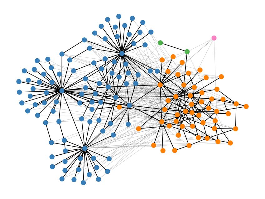
https://logeion.uchicago.edu/.C1 C2 full
Figure 1: Usage graph of Swedish ledning. D1 = (58, 0, 4, 0), D2 = (52, 14, 5, 1), B(w) = 1 and
G(w) = 0.34.
In order to reduce the search space, we iterate over different values for the maximum number of clusters.
We also iterate over randomly as well as heuristically chosen initial clustering states.11
This way of clustering usage graphs has several advantages: (i) It finds the optimal number of clusters
on its own. (ii) It easily handles missing information (non-observed edges). (iii) It is robust to errors
by using the global information on the graph. That is, a wrong judgment can be outweighed by correct
ones. (iv) It directly optimizes an intuitive quality criterion on usage graphs. Many other clustering
algorithms such as Chinese Whispers (Biemann, 2006) make local decisions, so that the final solution
is not guaranteed to optimize a global criterion such as L. (v) By weighing each edge with its (shifted)
weight, L respects the gradedness of word meaning. That is, edges with |W (e)| ≈ 0 have less influence
on L than edges with |W (e)| ≈ 1.5. Finally, it showed superior performance to all other clustering
algorithms we tested in a simulation study. (See Appendix A.)
4.4 Change scores
A sense frequency distribution (SFD) encodes how often a word w occurs in each of its senses (McCarthy
et al., 2004; Lau et al., 2014, e.g.). From the clustering we obtain two SFDs D, E for a word w in the two
corpora C1 , C2 , where each cluster corresponds to one sense.12 Binary LSC for Subtask 1 of the word w
is then defined as
B(w) = 1 if for some i, Di ≤ k and Ei ≥ n,
or vice versa. (2)
B(w) = 0 else.
where Di and Ei are the frequencies of sense i in C1 , C2 and k, n are lower frequency thresholds aimed
to avoid that small random fluctuations in sense frequencies caused by sampling variability or annotation
error are misclassified as change (Schlechtweg and Schulte im Walde, 2020). According to Definition 2, a
word is classified as gaining a sense, if the sense is attested at most k times in the annotation sample from
C1 , but attested at least n times in the sample from C2 . (Similarly for words that lose a sense.) We set
k = 0, n = 1 for the smaller samples (≤ 30) in Latin and k = 2, n = 5 for the larger samples (≤ 100) in
English, German, Swedish. We make no distinction between words that gain vs. words that lose senses,
both fall into the change class. Equally, we make no distinction between words that gain/lose one sense vs.
words that gain/lose several senses.
For graded LSC in Subtask 2 we first normalize D and E to probability distributions P and Q by
dividing each element by the total sum of the frequencies of all senses in the respective distribution. The
degree of LSC of the word w is then defined as the Jensen-Shannon distance between the two normalized
frequency distributions:
G(w) = JSD(P, Q) (3)
11
We used mlrose to perform the clustering (Hayes, 2019).
12
The frequency for sense i in corpus C is given by the number of uses from C in the cluster corresponding to sense i.C1 C2 full
Figure 2: Usage graph of German Eintagsfliege. D1 = (12, 45, 0, 1), D2 = (85, 6, 1, 1), B(w) = 0 and
G(w) = 0.66.
where the Jensen-Shannon distance is the symmetrized square root of the Kullback-Leibler divergence
(Lin, 1991; Donoso and Sanchez, 2017). G(w) is symmetric, ranges between 0 and 1 and is high if P
and Q assign very different probabilities to the same senses. Note that B(w) and G(w) not necessarily
correspond to each other: a word w may show no binary change but high graded change, or vice versa.
4.5 Result
Figure 1 and Figure 2 show the annotated and clustered usage graphs for Swedish target ledning and
German target Eintagsfliege. Nodes represent uses of the target word. Edges represent the median of
relatedness judgments between uses (black/gray lines for positive/negative edges). Colors make clusters
(senses) inferred on the full graph. After splitting the full graph into the two time-specific subgraphs
for C1 , C2 we obtain the two sense frequency distributions D1 , D2 . From these we inferred the binary
and the graded change value. The two words represent semantic changes indicative of Subtask 1 and 2
respectively: ledning gains a sense with rather low frequency in C2 . Hence, it has binary change, but
low graded change. For Eintagsfliege, however, its two main senses exist in both C1 and C2 , while their
frequencies change dramatically. Hence, it has no binary change, but high graded change.
Find a summary of the annotation outcome for all languages and target words in Table 4. The final test
sets contain between 31 (Swedish) and 48 (German) target words. Throughout the annotation we excluded
several targets if they had a high number of ‘0’ judgments or needed a high number of further edges
to be annotated. As previous studies, we report the mean of Spearman correlations between annotator
judgments as agreement measure. Erk et al. (2013) and Schlechtweg et al. (2018) report agreement
scores between 0.55 and 0.68, which is comparable to our scores.13 The clustering loss is the value of L
(Definition 1) divided by the maximum possible loss on the respective graph. It gives a measure of how
well the graphs could be partitioned into clusters by the L criterion.
The class distribution (column ‘LSC’) for Subtask 1 differs per language as a result of several target
words being dropped during the annotation. In Latin the majority of target words have binary change,
while in Swedish the majority has no binary change. This is also reflected in the mean scores for graded
LSC in Subtask 2. Despite the excluded target words the frequency statistics are roughly balanced
(FRQd , FRQm ). However, we did not control the test sets for polysemy and there are strong correlations
for English, German and Swedish between graded change and polysemy in Subtask 2 (PLYm ). This
correlation reduces for binary change in Subtask 1 but is still moderate for English and Swedish and
remains high for German.
In total, roughly 100,000 judgments were made by annotators. For English/German/Swedish ≈ 50% of
the use pairs were annotated by more than one annotator. In total, the annotation cost roughly e 20,000
for 1,000 hours – twice as much as originally budgeted.
13
Note that because we spread disagreements from previous rounds in each round to further annotators, on average uses in
later rounds become much harder to judge, which has a negative effect on agreement. Hence, for comparability reasons we report
the agreement in the first round where no disagreement detection has taken place. The agreement across all rounds, calculated as
weighted mean of agreements is 0.52/0.60/-/0.58.5 Evaluation
All teams were allowed a total of 10 submissions, the best of which was kept for the final ranking in the
competition. Participants had to submit predictions for both subtasks and all languages. A submission’s
final score for each subtask was computed as the average performance across all four languages. During
the evaluation phase, the leaderboard was hidden, as per SemEval recommendation.
5.1 Scoring Measures
For Subtask 1 submitted predictions were evaluated against the hidden labels via accuracy, given that we
anticipated the class distribution for target words to be approximately balanced before the annotation.
Scores are bounded between 0 and 1. As the distribution turned out to be imbalanced for some languages,
we also report F1-score in Appendix C. For Subtask 2, we used Spearman’s rank-order correlation
coefficient ρ with the gold rank. Spearman’s ρ only considers the order of the words, the actual predicted
change values were not taken into account. Ties are corrected by assigning the average of the ranks that
would have been assigned to all the tied values to each value (e.g. two words sharing rank 1 both get
assigned rank 1.5). Scores are bounded between −1 (completely opposite to true ranking) and 1 (exact
match).
5.2 Baselines
For both subtasks, we have two baselines: (i) Normalized frequency difference (Freq. Baseline) first
calculates the frequency for each target word in each of the two corpora, normalizes it by the total corpus
frequency and then calculates the absolute difference between these values as a measure of change.
(ii) Count vectors with column intersection and cosine distance (Count Baseline) first learns vector
representations for each of the two corpora, then aligns them by intersecting their columns and measures
change by cosine distance between the two vectors for a target word. A Python implementation of both
these baselines was provided in the starting kit. A third baseline, for Subtask 1, is the majority class
prediction (Maj. Baseline), i.e., always predicting the ‘0’ class (no change).
6 Participating Systems
Thirty-three teams participated in the task, totaling 53 members. The teams submitted a total of 186
submissions. Given the large number of teams, we provide a summary of the systems in the body of
this paper. A more detailed description of each participating system for which a paper was submitted is
available in Appendix B. We also encourage the reader to read the full system description papers.
Participating models can be described as a combination of (i) a semantic representation, (ii) an alignment
technique and (iii) a change measure. Semantic representations are mainly average embeddings (type
embeddings) and contextualized embeddings (token embeddings). Token embeddings are often combined
with a clustering algorithm such as K-means, affinity propagation (Frey and Dueck, 2007), (H)DBSCAN,
GMM, or agglomerative clustering. One team uses a graph-based semantic network, one a topic model
and several teams also propose ensemble models. Alignment techniques include Orthogonal Procrustes
(Hamilton et al., 2016, OP), Vector Initialization (Kim et al., 2014, VI), versions of Temporal Referencing
(Dubossarsky et al., 2019, TR), and Canonical Correlation Analysis (CCA). A variety of change measures
are applied, including Cosine Distance (CD), Euclidean Distance (ED), Local Neighborhood Distance
(LND), Kullback-Leibler Divergence (KLD), mean/standard deviation of co-occurrence vectors, or cluster
frequency. Table 5 shows the type of system for every team’s best submission for both subtasks.
7 Results
As illustrated by Table 5, UWB has the best performance in Subtask 1 for the average over all lan-
guages, closely followed by Life-Language, Jiaxin & Jinan14 and RPI-Trust.15 For Subtask 2,
14
The team is named “LYNX” on the competition CodaLab.
15
The team submits an ensemble model. As all of the features are derived from the type vectors, we classify it as “type” in this
section.Subtask 1 Subtask 2
Team System Team System
Avg. EN DE LA SV Avg. EN DE LA SV
UWB .687 .622 .750 .700 .677 type UG Student Intern .527 .422 .725 .412 .547 type
Life-Language .686 .703 .750 .550 .742 type Jiaxin & Jinan .518 .325 .717 .440 .588 type
Jiaxin & Jinan .665 .649 .729 .700 .581 type cs2020 .503 .375 .702 .399 .536 type
RPI-Trust .660 .649 .750 .500 .742 type UWB .481 .367 .697 .254 .604 type
UG Student Intern .639 .568 .729 .550 .710 type Discovery Team .442 .361 .603 .460 .343 ens.
DCC .637 .649 .667 .525 .710 type RPI-Trust .427 .228 .520 .462 .498 type
NLP@IDSIA .637 .622 .625 .625 .677 token Skurt .374 .209 .656 .399 .234 token
JCT .636 .649 .688 .500 .710 type IMS .372 .301 .659 .098 .432 type
Skurt .629 .568 .562 .675 .710 token UiO-UvA .370 .136 .695 .370 .278 token
Discovery Team .621 .568 .688 .550 .677 ens. Entity .352 .250 .499 .303 .357 type
Count Bas. .613 .595 .688 .525 .645 - Random .296 .211 .337 .253 .385 type
TUE .612 .568 .583 .650 .645 token NLPCR .287 .436 .446 .151 .114 token
Entity .599 .676 .667 .475 .581 type JCT .254 .014 .506 .419 .078 type
IMS .598 .541 .688 .550 .613 type cbk .234 .059 .400 .341 .136 token
cs2020 .587 .595 .500 .575 .677 token UCD .234 .307 .216 .069 .344 graph
UiO-UvA .587 .541 .646 .450 .710 token Life-Language .218 .299 .208 -.024 .391 type
NLPCR .584 .730 .542 .450 .613 token NLP@IDSIA .194 .028 .176 .253 .321 token
Maj. Bas. .576 .568 .646 .350 .742 - Count Bas. .144 .022 .216 .359 -.022 -
cbk .554 .568 .625 .475 .548 token UoB .100 .105 .220 -.024 .102 topic
Random .554 .486 .479 .475 .774 type RIJP .087 .157 .099 .065 .028 type
UoB .526 .568 .479 .575 .484 topic TUE .087 -.155 .388 .177 -.062 token
UCD .521 .622 .500 .350 .613 graph DCC -.083 -.217 .014 .020 -.150 type
RIJP .511 .541 .500 .550 .452 type Freq. Bas. -.083 -.217 .014 .020 -.150 -
Freq. Bas. .439 .432 .417 .650 .258 - Maj. Bas. - - - - - -
Table 5: Summary of the performance of systems for which a system description paper was submitted, as
well as their type of semantic representation for that specific submission in Subtask 1 (left) and Subtask 2
(right). For each team, we report the values of accuracy (Subtask 1) and Spearman correlation (Subtask 2)
corresponding to their best submission in the evaluation phase. Abbreviations: Avg. = average across
languages, EN = English, DE = German, LA = Latin, and SV = Swedish, type = average embeddings,
token = contextualised embeddings, topic = topic model, ens. = ensemble, graph = graph, UCD =
University College Dublin.
UG Student Intern performs best, followed by Jiaxin & Jinan and cs2020.16 Across all systems,
good performance in Subtask 1 does not indicate good performance in Subtask 2 (correlation between
the system ranks is 0.22). However, and with the exception of Life-Language and cs2020, most top
performing systems in Subtask 1 also excel in Subtask 2, albeit with a slight change of ranking.
Remarkably, all the top performing systems use static-type embedding models, and differ only in
terms of their solutions to the alignment problem (Canonical Correlation Analysis, Orthogonal Procrustes,
or Temporal Referencing). Interestingly, the top systems refine their models using one or more of the
following steps: a) computing additional features from the embedding space; b) combining scores from
different models (or extracted features) using ensemble models; c) choosing a threshold for changed
words based on a distribution of change scores. We conjecture that these additional (and sometimes
very original) post-processing steps are crucial for these systems’ success. We now briefly describe the
top performing systems in terms of these three steps (for further details please see Appendix B). UWB
(SGNS+CCA+CD) sets the average change score as the threshold (c). Life-Language (SGNS) represents
words according to their distances to a set of stable pivot words in two unaligned spaces, and compares
their divergence relative to a distribution of change scores obtained from unstable pivot words (a+c). RPI-
Trust (SGNS+OP) extract features (a word’s cosine distance, change of distances to its nearest-neighbours
and change in frequency), transform each word’s feature to a CDF score, and averages these probabilities
(a+b+c). Jiaxin & Jinan (SGNS+TR+CD) fits the empirical cosine distance change scores to a Gamma
Quantile Threshold, and sets the 75% quantile as the threshold (c). UG Student Intern (SGNS+OP)
measures change using Euclidean distance instead of cosine distance. cs2020 uses SGNS+OP+CD only
16
The team is named “cs2020” and “cs2021” on the competition CodaLab. The combined number of submissions made by the
two teams did not exceed the limit of 10.as baseline method.
An important finding common to most systems is the difference between their performances across
the four languages – systems that excel in one language do not necessarily perform well in another. This
discrepancy may be due to a range of factors, including the difference in corpus size and the nature of the
corpus data, as well as the relative availability of resources in some languages such as English over others.
The Latin corpus, for example, covers a very long time span, and the lower performance of the systems
on this language may be explained by the fact that the techniques employed, especially word token/type
embeddings, have been developed for living languages and little research is available on their adaptation
to dead and ancient languages. In general, dead languages tend to pose additional challenges compared to
living languages (Piotrowski, 2012), due to a variety of factors, including their less-resourced status, lack
of native speakers, high linguistic variation and non-standardized spelling, and errors in Optical Character
Recognition (OCR). Other factors that should be investigated are data quality (Hill and Hengchen, 2019;
van Strien et al., 2020): while English and Latin are clean data, German and Swedish present notorious
OCR errors. The availability of tuned hyperparameters might have played a role as well: for German,
some teams report following prior work such as Schlechtweg et al. (2019). Finally, another factor for
the discrepancy in performance between languages for any given system is not related to the nature of
the systems nor of the data, but due to the fact that some teams focused on some languages, submitting
dummy results for the others.
Type versus token embeddings Tables 5 and 6 illustrate the gap in performance between type-based
embedding models and the token-based ones. Out of the best 10 systems in Subtask 1/Subtask 2, 7/8
systems are based on type embeddings compared to only 2/2 systems that are based on token embeddings
(same holds for each language individually). Contrary to the recent success of token embeddings (Peters
et al., 2018) and to commonly held view that contextual embeddings “do everything better”, they are
overwhelmingly outperformed by type embeddings in our task. This is most surprising for Subtask 1,
because type embeddings do not distinguish between different senses, while token embeddings do. We
suggest several possible reasons for these surprising results. The first is the fact that contextual embedding
is a recent technology, and as such lacks proper usage conventions. For example, it is not clear whether a
model should create an average token representation based on individual instances (and if so, which layers
should be averaged), or if it should use clustering of individual instances instead (and if so, what type of
clustering algorithm etc.). A second reason may be related to the fact that contextual models are pretrained
and cannot exclusively be trained on the relevant historical resources (in contrast to type embeddings). As
such, they carry additional, and possibly irrelevant, information that may mask true diachronic changes.
The results may also be related to the specific preprocessing we applied to the corpora: (i) Only restricted
context is available to the models as a result of the sentence shuffling. Usually, token-based models take
more context into account than just the immediate sentence (Martinc et al., 2020). (ii) The corpora were
lemmatized, while token-based models usually take the raw sentence as input. In order to make the input
more suitable for token-based models, we also provide the raw corpora after the evaluation phase and will
publish the annotated uses of the target words with additional context.17
The influence of frequency In prior work, the predictions of many systems have been shown to be
inherently biased towards word frequency, either as a consequence of an increasing sampling error
with lower frequency (Dubossarsky et al., 2017) or by directly relying on frequency-related variables
(Schlechtweg et al., 2017; Schlechtweg et al., 2019). We have controlled for frequency when selecting
target words (recall Table 4) in order to test model performance when frequency is not an indicating
factor. Despite the controlled test sets we observe strong frequency biases for the individual models as
illustrated for Swedish in Figure 3.18 Models rather correlate negatively with the minimum frequency of
target words between corpora (FRQm ), and positively with the change in their frequency across corpora
(FRQd ). This means that models predict higher change for low-frequency words and higher change for
words with strong changes in frequency. Despite their superior performance, type embeddings are more
17
https://www.ims.uni-stuttgart.de/data/sem-eval-ulscd
18
Find the full set of analysis plots at https://www.ims.uni-stuttgart.de/data/sem-eval-ulscd-post.Subtask 1 Subtask 2
System
Avg. Max. Avg. Max.
type embeddings 0.625 0.687 0.329 0.527
ensemble 0.621 0.621 0.442 0.442
token embeddings 0.598 0.637 0.258 0.374
topic model 0.526 0.526 0.100 0.100
graph 0.521 0.521 0.234 0.234
Table 6: Average and maximum performance of best submissions per subtask for different system types.
Submissions that corresponded exactly to the baselines or the sample submission were removed.
Figure 3: Influence of frequency on model predictions in Subtask 2, Swedish. X-axis: correlations with
FRQd (left) and FRQm (right), Y-axis: performance on Subtask 2. Gray line gives frequency correlation
in gold data.
strongly influenced by frequency than token embeddings, probably because the latter are not trained on
the test corpora limiting the influence of frequency. Similar tendencies can be seen for the other languages.
For a range of models correlations reach values > 0.8.
The influence of polysemy We did not control the test sets for polysemy. As shown in Table 4, the
change scores for both subtasks are moderately to highly correlated with polysemy (PLYm ). Hence, it
is expected that model predictions would be positively correlated with polysemy. However, these are
in almost all cases lower than for the change scores and in some cases even negative (Latin and partly
English). We conclude that model predictions are only moderately biased towards polysemy on our data.
Prediction difficulty of words In order to quantify how difficult a target word is to predict we compute
the mean error of all participants’ predictions.19 In Subtask 1, we find that words with higher rank tend
to have higher error, in particular for English, see Figure 4 (left) where words with the gold class 1
have almost twice as high average error than words with gold class 0, and Latin. This is likely due to
the tendency for systems to provide zero-predictions following the published baselines. For Subtask 2
(right), we find that the opposite holds; stable words are harder to predict for all languages but Swedish,
where instead, it seems that the words in the middle of the rank are the hardest to classify. For English,
the top three hardest to predict words are for Subtask 1 vs. Subtask 2 are land, head, edge vs. word,
head, multitude. For German, they are packen, überspannen, abgebrüht vs. packen, Seminar, vorliegen.
For Latin, they are cohors, credo, virtus vs. virtus, fidelis, itero. For Swedish, they are kemisk, central,
bearbeta vs. central, färg, blockera. We could not identify a general pattern with regards to these words’
frequency or polysemy properties.
19
Because Subtask 2 is a ranking task, we divide the mean error by the expected error: since words in the middle have a lower
expected error than words in the top or bottom.Figure 4: Normalized prediction errors for Subtask 1, English (left) and Subtask 2, German (right). 8 Conclusion We presented the results of the first shared task on Unsupervised Lexical Semantic Change Detection. A wide range of systems were evaluated on two subtasks in four languages relying on a thoroughly annotated data set based on ∼100,000 human judgments. The task setup (unsupervised, no genuine development data, different corpora from different languages with very different sizes, varying class distributions) provided an opportunity to test models in heterogeneous learning scenarios, that was very challenging. Hence, both subtasks remain far from solved. However, several teams reach high performances on both subtasks. Surprisingly, type embeddings outperformed token embeddings on both subtasks. We suspect that the potential of token embeddings has not yet fully unfolded, as no canonical application concept is available and preprocessing was not optimal for token embeddings. We found that type embeddings are strongly influenced by frequency. Hence, one important challenge for future type-based models will be to avoid the frequency bias stemming from the corpus on which they are trained. An important challenge for token-based models will be to understand the reasons for their current low performance and to develop robust ways for their application. We found that change scores in our test sets strongly correlate with polysemy, despite model predictions not showing such strong influence. We believe that this should be pursued in the future by controlling test sets for polysemy. We hope that SemEval-2020 Task 1 makes a lasting contribution to the field of Unsupervised Lexical Semantic Change Detection by providing researchers with a standard evaluation framework and high- quality data sets. Despite the limited size of the test sets, many previously reached conclusions can now be tested more thoroughly and future models can be compared on a shared benchmark. The current test set can also be used to test models that have been trained on the full data available for the participating corpora. Data from additional time periods can be utilized by models that need finer granularity for detection, while testing on the two time periods available in the current test sets. Acknowledgments The authors would like to thank Dr. Diana McCarthy for her valuable input to the genesis of this task. DS was supported by the Konrad Adenauer Foundation and the CRETA center funded by the German Ministry for Education and Research (BMBF) during the conduct of this study. This task has been funded in part by the project Towards Computational Lexical Semantic Change Detection supported by the Swedish Research Council (2019–2022; dnr 2018-01184), and Nationella språkbanken (the Swedish National Language Bank) – jointly funded by (2018–2024; dnr 2017-00626) and its 10 partner institutions, to NT. The list of potential change words in Swedish was provided by the research group at the Department of Swedish, University of Gothenburg that works with the Contemporary Dictionary of the Swedish Academy. This work was supported by The Alan Turing Institute under the EPSRC grant EP/N510129/1, to BMcG. Additional thanks go to the annotators of our datasets, and an anonymous donor.
References
Yvonne Adesam, Dana Dannélls, and Nina Tahmasebi. 2019. Exploring the quality of the digital historical
  newspaper archive KubHist. In Proceedings of the 2019 DHN conference, pages 9–17.
Reem Alatrash, Dominik Schlechtweg, Jonas Kuhn, and Sabine Schulte im Walde. 2020. CCOHA: Clean Corpus
  of Historical American English. In Proceedings of the Twelfth International Conference on Language Resources
  and Evaluation (LREC’20). European Language Resources Association (ELRA).
Efrat Amar and Chaya Liebeskind. 2020. JCT at SemEval-2020 Task 1: Combined Semantic Vector Spaces Mod-
  els for Unsupervised Lexical Semantic Change Detection. In Proceedings of the 14th International Workshop
  on Semantic Evaluation, Barcelona, Spain. Association for Computational Linguistics.
Asaf Amrami and Yoav Goldberg. 2018. Word sense induction with neural bilm and symmetric patterns. arXiv
  preprint arXiv:1808.08518.
Asaf Amrami and Yoav Goldberg. 2019. Towards better substitution-based word sense induction. arXiv preprint
  arXiv:1905.12598.

Nikolay Arefyev and Vasily Zhikov. 2020. BOS at SemEval-2020 Task 1: Word Sense Induction via Lexical
  Substitution for Lexical Semantic Change Detection. In Proceedings of the 14th International Workshop on
  Semantic Evaluation, Barcelona, Spain. Association for Computational Linguistics.

Mikel Artetxe, Gorka Labaka, and Eneko Agirre. 2018. A robust self-learning method for fully unsupervised
  cross-lingual mappings of word embeddings. In Proceedings of the 56th Annual Meeting of the Association for
  Computational Linguistics (Volume 1: Long Papers), pages 789–798, Melbourne, Australia, July. Association
  for Computational Linguistics.

Ehsaneddin Asgari, Christoph Ringlstetter, and Hinrich Schütze. 2020. EmbLexChange at SemEval-2020 Task 1:
  Unsupervised Embedding-based Detection of Lexical Semantic Changes. In Proceedings of the 14th Interna-
  tional Workshop on Semantic Evaluation, Barcelona, Spain. Association for Computational Linguistics.
Nikhil Bansal, Avrim Blum, and Shuchi Chawla. 2004. Correlation clustering. Machine Learning, 56(1-3):89–
  113.
Pierpaolo Basile, Annalina Caputo, and Giovanni Semeraro. 2015. Temporal random indexing: A system for
   analysing word meaning over time. Italian Journal of Computational Linguistics, 1(1):55–68.
Christin Beck. 2020. DiaSense at SemEval-2020 Task 1: Modeling sense change via pre-trained BERT embed-
  dings. In Proceedings of the 14th International Workshop on Semantic Evaluation, Barcelona, Spain. Associa-
  tion for Computational Linguistics.
Berliner Zeitung. 2018. Diachronic newspaper corpus published by Staatsbibliothek zu Berlin.

Chris Biemann. 2006. Chinese whispers: An efficient graph clustering algorithm and its application to natural
  language processing problems. In Proceedings of the First Workshop on Graph Based Methods for Natural
  Language Processing, TextGraphs-1, page 73–80, USA. Association for Computational Linguistics.

Chris Biemann. 2013. Creating a system for lexical substitutions from scratch using crowdsourcing. Lang. Resour.
  Eval., 47(1):97–122, March.
Andreas Blank. 1997. Prinzipien des lexikalischen Bedeutungswandels am Beispiel der romanischen Sprachen.
  Niemeyer, Tübingen.
Vincent D. Blondel, Jean-Loup Guillaume, Renaud Lambiotte, and Etienne Lefebvre. 2008. Fast unfolding of
  communities in large networks. Journal of Statistical Mechanics: Theory and Experiment, 2008(10):10008,
  October.
Lars Borin, Markus Forsberg, and Johan Roxendal. 2012. Korp — the corpus infrastructure of Språkbanken. In
  Proceedings of the Eighth International Conference on Language Resources and Evaluation (LREC’12), pages
  474–478, Istanbul, Turkey, May. European Language Resources Association (ELRA).
Pierluigi Cassotti, Annalina Caputo, Marco Polignano, and Pierpaolo Basile. 2020. GM-CTSC at SemEval-2020
   Task 1: Gaussian Mixtures Cross Temporal Similarity Clustering. In Proceedings of the 14th International
  Workshop on Semantic Evaluation, Barcelona, Spain. Association for Computational Linguistics.
Wanxiang Che, Yijia Liu, Yuxuan Wang, Bo Zheng, and Ting Liu. 2018. Towards better ud parsing: Deep
  contextualized word embeddings, ensemble, and treebank concatenation. In Proceedings of the CoNLL 2018
 Shared Task: Multilingual Parsing from Raw Text to Universal Dependencies, pages 55–64.
James Clackson. 2011. A Companion to the Latin Language. Wiley-Blackwell.

Alexis Conneau, Kartikay Khandelwal, Naman Goyal, Vishrav Chaudhary, Guillaume Wenzek, Francisco Guzmán,
  Edouard Grave, Myle Ott, Luke Zettlemoyer, and Veselin Stoyanov. 2019. Unsupervised cross-lingual repre-
  sentation learning at scale. arXiv preprint arXiv:1911.02116.

Paul Cook, Jey Han Lau, Diana McCarthy, and Timothy Baldwin. 2014. Novel word-sense identification. In
  Proceedings of COLING 2014, the 25th International Conference on Computational Linguistics: Technical
  Papers, pages 1624–1635.
Mark Davies. 2012. Expanding Horizons in Historical Linguistics with the 400-Million Word Corpus of Historical
 American English. Corpora, 7(2):121–157.
Deutsches Textarchiv. 2017. Grundlage für ein Referenzkorpus der neuhochdeutschen Sprache. Herausgegeben
  von der Berlin-Brandenburgischen Akademie der Wissenschaften.
Jacob Devlin, Ming-Wei Chang, Kenton Lee, and Kristina Toutanova. 2019. BERT: Pre-training of deep bidirec-
   tional transformers for language understanding. In Proceedings of the 2019 Conference of the North American
   Chapter of the Association for Computational Linguistics: Human Language Technologies, Volume 1 (Long and
   Short Papers), pages 4171–4186, Minneapolis, Minnesota, June. Association for Computational Linguistics.
Gonzalo Donoso and David Sanchez. 2017. Dialectometric analysis of language variation in Twitter. CoRR,
  abs/1702.06777.
Haim Dubossarsky, Daphna Weinshall, and Eitan Grossman. 2017. Outta control: Laws of semantic change and
  inherent biases in word representation models. In Proceedings of the 2017 Conference on Empirical Methods
  in Natural Language Processing, pages 1147–1156, Copenhagen, Denmark.
Haim Dubossarsky, Simon Hengchen, Nina Tahmasebi, and Dominik Schlechtweg. 2019. Time-Out: Temporal
  Referencing for Robust Modeling of Lexical Semantic Change. In Proceedings of the 57th Annual Meeting of
  the Association for Computational Linguistics, pages 457–470, Florence, Italy. Association for Computational
  Linguistics.
Katrin Erk, Diana McCarthy, and Nicholas Gaylord. 2013. Measuring word meaning in context. Computational
  Linguistics, 39(3):511–554.

Brendan J. Frey and Delbert Dueck. 2007. Clustering by passing messages between data points. Science,
  315(5814):972–976.

Maurı́cio Gruppi, Sibel Adalı, and Pin-Yu Chen. 2020. SChME at SemEval-2020 Task 1: A Model Ensem-
 ble for Detecting Lexical Semantic Change. In Proceedings of the 14th International Workshop on Semantic
 Evaluation, Barcelona, Spain. Association for Computational Linguistics.
Amaru Cuba Gyllensten, Evangelia Gogoulou, Ariel Ekgren, and Magnus Sahlgren. 2020. SenseCluster at
 SemEval-2020 Task 1: Unsupervised Lexical Semantic Change Detection. In Proceedings of the 14th Inter-
 national Workshop on Semantic Evaluation, Barcelona, Spain. Association for Computational Linguistics.
William L. Hamilton, Jure Leskovec, and Dan Jurafsky. 2016. Diachronic word embeddings reveal statistical
  laws of semantic change. In Proceedings of the 54th Annual Meeting of the Association for Computational
  Linguistics (Volume 1: Long Papers), pages 1489–1501, Berlin, Germany.
Anna Hätty, Dominik Schlechtweg, and Sabine Schulte im Walde. 2019. SURel: A gold standard for incorporating
  meaning shifts into term extraction. In Proceedings of the 8th Joint Conference on Lexical and Computational
  Semantics, pages 1–8, Minneapolis, MN, USA.
Genevieve Hayes. 2019. mlrose: Machine Learning, Randomized Optimization and SEarch package for Python.
  https://github.com/gkhayes/mlrose. Accessed: May 22, 2020.
Simon Hengchen, Ruben Ros, Jani Marjanen, and Mikko Tolonen. to appear. A data-driven approach to studying
  changing vocabularies in historical newspaper collections. Digital Scholarship in the Humanities.
Mark J Hill and Simon Hengchen. 2019. Quantifying the impact of dirty OCR on historical text analysis: Eigh-
 teenth Century Collections Online as a case study. Digital Scholarship in the Humanities, 34(4):825–843.
Ran Iwamoto and Masahiro Yukawa. 2020. RIJP at SemEval-2020 Task 1: Gaussian-based Embeddings for
  Semantic Change Detection. In Proceedings of the 14th International Workshop on Semantic Evaluation,
  Barcelona, Spain. Association for Computational Linguistics.
Vaibhav Jain. 2020. GloVeInit at SemEval-2020 Task 1: Using GloVe Vector Initialization for Unsupervised Lex-
  ical Semantic Change Detection. In Proceedings of the 14th International Workshop on Semantic Evaluation,
  Barcelona, Spain. Association for Computational Linguistics.
Vani K, Sandra Mitrović, Alessandro Antonucci, and Fabio Rinaldi. 2020. SST-BERT at SemEval-2020 Task 1:
  Semantic Shift Tracing by Clustering in BERT-based Embedding Spaces. In Proceedings of the 14th Interna-
  tional Workshop on Semantic Evaluation, Barcelona, Spain. Association for Computational Linguistics.
Jens Kaiser, Dominik Schlechtweg, Sean Papay, and Sabine Schulte im Walde. 2020. IMS at SemEval-2020 Task
  1: How low can you go? Dimensionality in Lexical Semantic Change Detection. In Proceedings of the 14th
  International Workshop on Semantic Evaluation, Barcelona, Spain. Association for Computational Linguistics.
Anna Karnysheva and Pia Schwarz. 2020. TUE at SemEval-2020 Task 1: Detecting semantic change by clustering
  contextual word embeddings. In Proceedings of the 14th International Workshop on Semantic Evaluation,
  Barcelona, Spain. Association for Computational Linguistics.
Yoon Kim, Yi-I Chiu, Kentaro Hanaki, Darshan Hegde, and Slav Petrov. 2014. Temporal analysis of language
  through neural language models. In LTCSS@ACL, pages 61–65. Association for Computational Linguistics.
Andrey Kutuzov and Mario Giulianelli. 2020. UiO-UvA at SemEval-2020 Task 1: Contextualised Embeddings
  for Lexical Semantic Change Detection. In Proceedings of the 14th International Workshop on Semantic Eval-
  uation, Barcelona, Spain. Association for Computational Linguistics.
Andrey Kutuzov, Lilja Øvrelid, Terrence Szymanski, and Erik Velldal. 2018. Diachronic word embeddings and
  semantic shifts: A survey. In Proceedings of the 27th International Conference on Computational Linguistics,
  pages 1384–1397, Santa Fe, New Mexico, USA. Association for Computational Linguistics.
Jey Han Lau, Paul Cook, Diana McCarthy, Spandana Gella, and Timothy Baldwin. 2014. Learning word sense
   distributions, detecting unattested senses and identifying novel senses using topic models. In Proceedings of
   the 52nd Annual Meeting of the Association for Computational Linguistics (Volume 1: Long Papers), pages
   259–270, Baltimore, Maryland, June. Association for Computational Linguistics.
Jianhua Lin. 1991. Divergence measures based on the Shannon entropy. IEEE Transactions on Information
   theory, 37(1):145–151.
Matej Martinc, Syrielle Montariol, Elaine Zosa, and Lidia Pivovarova. 2020. Discovery Team at SemEval-2020
 Task 1: Context-sensitive Embeddings not Always Better Than Static for Semantic Change Detection. In Pro-
 ceedings of the 14th International Workshop on Semantic Evaluation, Barcelona, Spain. Association for Com-
 putational Linguistics.
Diana McCarthy, Rob Koeling, Julie Weeds, and John Carroll. 2004. Finding predominant word senses in un-
  tagged text. In Proceedings of the 42nd Meeting of the Association for Computational Linguistics (ACL’04),
  Main Volume, pages 279–286, Barcelona, Spain, July.
Barbara McGillivray and Adam Kilgarriff. 2013. Tools for historical corpus research, and a corpus of Latin. In
  Paul Bennett, Martin Durrell, Silke Scheible, and Richard J. Whitt, editors, New Methods in Historical Corpus
  Linguistics, Tübingen. Narr.
Barbara McGillivray, Simon Hengchen, Viivi Lähteenoja, Marco Palma, and Alessandro Vatri. 2019. A computa-
  tional approach to lexical polysemy in Ancient Greek. Digital Scholarship in the Humanities, 34(4):893–907.
Tomas Mikolov, Kai Chen, Greg Corrado, and Jeffrey Dean. 2013a. Efficient estimation of word representa-
  tions in vector space. In Yoshua Bengio and Yann LeCun, editors, 1st International Conference on Learning
  Representations, ICLR 2013, Scottsdale, Arizona, USA, May 2-4, 2013, Workshop Track Proceedings.
Tomas Mikolov, Ilya Sutskever, Kai Chen, Greg Corrado, and Jeffrey Dean. 2013b. Distributed representations of
  words and phrases and their compositionality. In Proceedings of NIPS.
Neues Deutschland. 2018. Diachronic newspaper corpus published by Staatsbibliothek zu Berlin.
Paul Nulty and David Lillis. 2020. The UCD-Net System at SemEval-2020 Task 1: Temporal Referencing with
  Semantic Network Distances. In Proceedings of the 14th International Workshop on Semantic Evaluation,
  Barcelona, Spain. Association for Computational Linguistics.
You can also read