Single particle diffusion characterization by deep learning - bioRxiv

Single particle diffusion characterization by deep learning

 Naor Granik1,2, Lucien E. Weiss1,2, Maayan Shalom3, Michael Chein4, Eran Perlson4, Yael
 Roichman3,5, Yoav Shechtman1,2
1
 Department of Biomedical Engineering, Technion - Israel Institute of Technology, Haifa 3200003, Israel
2
 Lorry Lokey Interdisciplinary Center for Life Sciences and Engineering, Technion - Israel Institute of
Technology, Haifa 3200003, Israel
3
 Raymond & Beverly Sackler School of Chemistry, Tel Aviv University, Tel Aviv 6997801, Israel
4
 Department of Physiology and Pharmacology, Sackler Faculty of Medicine, and Sagol School of Neuroscience,
Tel Aviv University
5
 Raymond & Beverly Sackler School of Physics, Tel Aviv University, Tel Aviv 6997801, Israel

Corresponding: yoavsh@bm.techinon.ac.il, roichman@tauex.tau.ac.il

Table of contents

 1. CNN network architecture
 2. SNR definition
 3. Classification network – additional results
 a. Confusion matrices
 b. Classification performance with Ornstein-Uhlenbeck noise
 c. Classification of experimental data – beads in glycerol solution
 d. Classification of experimental data – Protein diffusion
 4. H regression network – additional results
 5. Multi-Track network – additional results
 6. D regression network – data conversion
 7. Beads in glycerol experiments
 a. Theoretical calculation
 b. Movie S1
 8. Materials and methods
 a. Fluorescent beads in F-actin networks
 b. Fluorescent beads in Glycerol solution

1. CNN network architecture

Network architecture is based on the design shown in (1). Four sets of convolution blocks with
different filter sizes [2,3,4,10], operate in parallel (Fig S1A). Each block consists of 1D dilated causal
convolution layers with increasing dilation factors (Fig S1B). This setup was designed to find
correlations spanning multiple time scales of unknown length. This architecture was selected in a
process of trial and error, based on classification and regression performance on simulated data.
Additional convolution layers were added or removed according to the track size a specific network
was intended for. For example, the network designed for 1000-step tracks has an additional
convolution block with filter size of 20.

 For the Multi-Track networks, the 1D convolution layers were replaced by 2D convolution
layers with dilation factors operating on the temporal axis only (i.e. for an input matrix M with the
shape [Number of tracks][Number of steps] the dilation factor will be (1,d)).

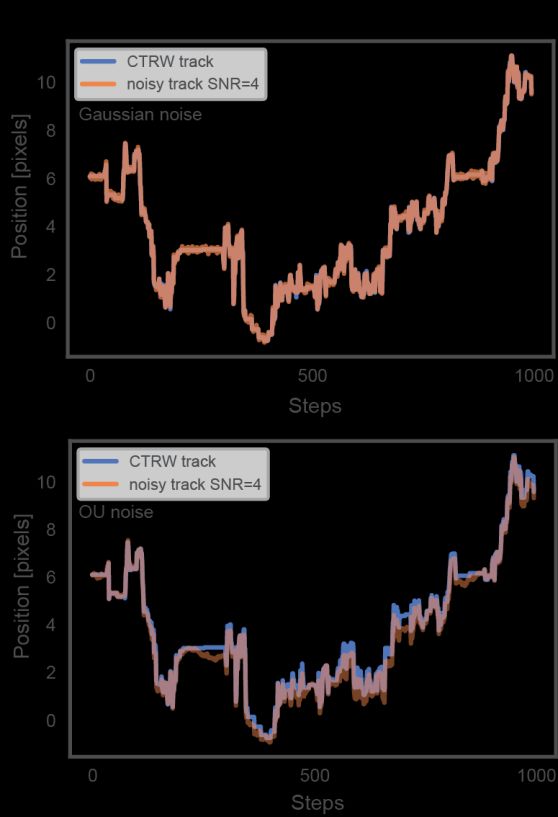
Networks were implemented and trained using Keras (Version 2.2.4) with TensorFlow
backend version (1.8.0) in Python (version 3.5). Other packages used: NumPy (version 1.14.5), SciPy
(version 1.2.1), Stochastic (version 0.4). Training was done on NVIDIA GeForce Titan GTX in a Windows
environment.

 FIGURE S1. Neural network architecture. A. Schematic of the neural network basic structure. B. An example convolution block with
 filter size = 2 and dilation factors = 1,2,4.

 2. SNR definitions

 Localization noise: For a trajectory , we
 define the Signal to Noise Ratio (SNR) as the
 ratio between the standard deviation of the
 signal increments to the standard deviation of
 the Gaussian noise added to the signal.
 
 ( )
 ≜ 
 ( )
 For , a zero mean Gaussian process.

 A second noise process which we consider is
 the Ornstein-Uhlenbeck (OU) noise, which can
 reflect environmental noise (i.e. an active
 environent “pushing” against the diffusing
 particle) (2, 3).

 In simple terms, an OU process can be
 considered as a Brownian motion with an
 additional feedback relaxation to a mean
 FIGURE S2. Sample noisy tracks. a. CTRW track (blue) with added position . Mathematically, is an OU
 Gaussian noise(orange), SNR = 4. b. CTRW track (blue) with added process if it satisfies the following stochastic
 OU noise (orange). SNR = 4
 differential equation:

 = ( − ) + 
With a zero mean Gaussian process. – speed of relaxation; – mean of the process; –
volatility of the process.

We consider an OU process with = 0, = = 1. For a trajectory , we define the noisy trajectory
as:

 = + , ≥ 0

and the SNR as:
 1
 =
 
3. Classification network - additional results

a. Confusion matrices

Classification confusion tables presented are organized according to SNR levels and are all based on
simulated tracks of 100 steps. Tables were produced by simulating a set of 300 tracks, 100 for each
diffusion model. Parameters for CTRW and FBM were selected at random from the range of values
that should not result in Brownian motion ( ∈ [0.05,0.9], ∈ [0.05,0.45] ∪ [0.55,0.95]), in order to
maintain correct statistics in the data set.

 Ground truth
 SNR = ∞
 FBM Brownian CTRW
 FBM 84 14 2
 Network prediction Brownian 0 99 1
 CTRW 5 2 93

 Ground truth
 SNR = 
 FBM Brownian CTRW
 FBM 82 16 2
 Network prediction Brownian 0 99 1
 CTRW 6 3 91

 Ground truth
 SNR = 
 FBM Brownian CTRW
 FBM 80 17 3
 Network prediction Brownian 0 99 1
 CTRW 9 5 86

 Ground truth
 SNR = 
 FBM Brownian CTRW
 FBM 77 20 3
 Network prediction Brownian 26 74 0
 CTRW 28 12 60

 Ground truth
 SNR = 
 FBM Brownian CTRW
 FBM 67 31 2
 Network prediction Brownian 99 1 0
 CTRW 69 23 8

The confusion matrices show the identification network is accurate even at relatively low SNR levels,
beginning to falter at SNR=2. Another important result is the uncertainty between FBM and Brownian
motion, even with no addition noise. This is caused by the fact that FBM is a generalization of Brownian
motion, with certain parameter choices causing the network to err between the two. This is true

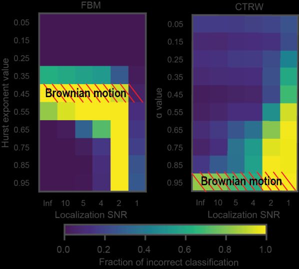
despite the fact that the Brownian motion parameter range – [0.45-0.55] was not used during
generation of the dataset.

To illustrate this, we show below the confusion table for SNR=∞, but for a data set wherein H was
selected from the parameter range – [0.05,0.35] ∪ [0.65,0.95].

 SNR = ∞ Ground truth
 FBM Brownian CTRW
 Reduced H range
 FBM 93 7 0
 Network prediction Brownian 0 100 0
 CTRW 8 1 91
An additional result arising from the above tables, is that there is no noticeable ambiguity between
CTRW and Brownian motion. This possibly has less to do with parameter choices, but rather with the
features the neural network learns. During the training phase, each filter learns different features of
the signal, CTRW is characterized by long waiting periods between jumps, which results in the diffusing
particle being noticeably ‘stuck’ in its position. It is highly likely that the network found this significant,
resulting in signals in which there is some evidence of a stuck particle being classified as CTRW. A
further indication to this can be found in the confusion table for SNR=1, in which the additional noise
masks the signal itself, making it similar to FBM.

b. Classification accuracy with Ornstein-Uhlenbeck noise

 Figure S3 presents the fraction of wrong
 predictions as a function of parameter and SNR.
 For CTRW, the network performs well up to SNR
 of 4, where it begins to falter, reverting to FBM
 due to the additional noise process, however for
 low values of , the network retains its CTRW
 prediction.
 For FBM, we see similar behavior to the case of
 Gaussian localization noise, with the exception
 of SNR = 1, where we see evidence that the noise
 process is a fractional Gaussian process,
 comparable to FBM (3).

 To further illustrate this, presented below are
 two confusion matrices for SNR = 5,1.
 FIGURE S3: Model identification (classification) network with
 additional OU noise. Heat maps presenting fraction of classification
 errors as a function of model parameter and OU-SNR. Each pixel
 represents results from 200 simulated trajectories.

 Ground truth
 SNR = 
 FBM Brownian CTRW
 FBM 86 14 0
 Network prediction Brownian 0 99 1
 CTRW 9 5 86

Ground truth
 SNR = 
 FBM Brownian CTRW
 FBM 91 7 2
 Network prediction Brownian 97 3 0
 CTRW 62 7 31

c. Classification of experimental data set – beads diffusing in glycerol solution

 Figure S4 shows classification results for the experimental
 bead-in-glycerol data. As can be seen, the classification is
 not perfect, showing nearly similar numbers of FBM and
 Brownian motion (the minor CTRW population represents
 beads stuck to the surface unable to move, these do not
 appear in the H-estimation analysis). The fault most likely
 lies in a combination of precision errors and other
 unknown factors relating to the experiment (e.g. effects of
 fluid dynamics). Analysis using H network shows a
 population centered around H = 0.6 with standard
 deviation of 0.07, in agreement with the classification
 results (i.e. approximately half classified as FBM, and half
 as Brownian motion).

 FIGURE S4: Classification of experimental
 data – beads diffusing in glycerol. Top:
 Classification results. Bottom: analysis of
 same data by H-network based on 100 steps.

d. Classification of experimental data set – Proteins diffusing on a membrane surface

 This experiment presents a unique challenge in that the
 motion does not fit into any one anomalous diffusion
 model. For this reason, we cannot simply set the highest
 probability in the network output as the selected model,
 but instead must look at probabilities themselves. Fig. S5
 shows the 2D probability distribution space from 205
 experimental trajectories. X, Y axes represent probabilities
 of being assigned to FBM and CTRW models, respectively.
 The data closely follows a = − trend line, with clusters
 of tracks being scattered around (x,y) = (0.5,0.5), or (x,y) =
 (1,0) From this we can conclude: The network identifies
 features from both models, while almost entirely
 Figure S5: Classification of experimental data disregarding the Brownian motion model (otherwise the
 – Proteins diffusing on membrane surface. sum of and would not be one); The network
 Results presented are probabilities of being shows a bias towards FBM as was previously shown on
 identified as FBM model (x axis) or CTRW
 simulated data.
 model (y axis)

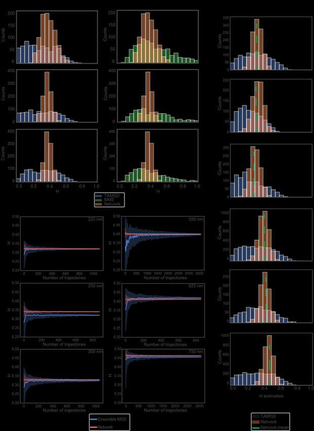
4. Hurst parameter regression network - additional results

 FIGURE S6: Additional H network results. A. Estimation of single value by TAMSD, MME and networks on tracks of different sizes.
 1000 different tracks were generated with H = 0.4 and SNR = 4 B+C. Experimental data – beads diffusing in Actin gel of different
 mesh sizes (sizes written in figure). B – Evaluation by TAMSD and network; C – Evaluation by ensemble MSD and network.

Figure S6-A presents a comparison between three methods – Mean Square Displacement (MSD),
Mean Maximal Excursion (MME) (4) and network estimation for three different track lengths. Tracks
were simulated with H = 0.4 and SNR = 4. Estimation is based on single tracks only. The results are
summarized in the following table:

 25-steps 100-steps 1000-steps
 Network 0.39 ± 0.08 0.37 ± 0.05 0.39 ± 0.04
 MSD 0.22 ± 0.21 0.29 ± 0.19 0.32 ± 0.17
 MME 0.55 ± 0.41 0.48 ± 0.31 0.45 ± 0.3

The results show that all three methods converge to an estimation of 0.4, as the tracks increase in
length, with the network outperforming MSD and MME in both accuracy and estimation standard
deviation.

Figure S5-B, C present the complete results for the experimental data summarized in the paper.
Comparing network estimation to time averaged MSD and ensemble MSD, respectively.

5. Multi-Track network - additional results

 FIGURE S7: Multi-Track network heat maps showing RMSE as function of Localization SNR and number of tracks used for MME,
 ensemble MSD and MT-network. Each pixel represents 200 simulations of Mx10-step-tracks generated, with M being the number of
 tracks corresponding to the value in the heat map x-axis.

6. Diffusion coefficient regression network - data conversion

D-network was defined to operate at a specific pixel size and frame length, 550nm and 0.05 seconds,
respectively. These settings were selected to fit available experimental data. Due to the nature of the
problem, input data cannot be standardized as this would effectively destroy the diffusion coefficient
information in the data. Despite this hard-coded setting, data from different setups can be entered
with two simple conversion steps.

Temporal conversion can be done post-analysis, on the diffusion coefficient results by the equation:
 0.05
 = ∙
 Δ 

Pixel size conversion must be done on the localization data, prior to calculating the mean and standard
deviation of increments, this is done by the equation:
 
 = ∙
 0.55

μ 2
Following conversion, the data can be entered to the network with the output being in 
 .

 2
FIGURE S8: Effect of pixel conversion. 200 Tracks were generated with = 1[ ], with pixel size setting of 200 nm per
 
pixel and analysed by the network and by temporal MSD. Left: Estimation of raw track data, without pixel size correction,
MSD was calculated with correct pixel size. Right: Estimation of track data with pixel conversion.

7. Beads in glycerol experiment

a. Theoretical calculations

Theoretical diffusion coefficient values for the diffusion-in-glycerol experiment were calculated using
the Stokes-Einstein equation for diffusion of spherical particles through a liquid with low Reynolds
number (5).
 
 =
 6 
Where:
 2
 – Diffusion coefficient [ 
 ]

 2 
 – Boltzmann constant [ ∙ 2
 ]

 – Temperature [ ]
 
 – Viscosity [ ∙ ]

 – Particle radius [ ]

The experiments were conducted in room temperature with beads of two different sizes -
 
100,200 [ ] in a solution of 40% glycerol in water, giving a viscosity coefficient of 0.00372 [ ∙ ] (6).

 1.3806 ∙ 10−23 ∙ 293 −13
 2 2
 100[ ] = = = 5.722 ∙ 10 [ ] = 0.57 [ ]
 6 6 ∙ 0.00372 ∙ 100 ∙ 10−9 

 1.3806 ∙ 10−23 ∙ 293 −13
 2 2
 200[ ] = = = 2.884 ∙ 10 [ ] = 0.28 [ ]
 6 6 ∙ 0.00372 ∙ 200 ∙ 10−9 

b. Supporting movie

Movie S1 depicts a sample experiment consisting of two populations of beads diffusing in 40%
Glycerol solution. Green and red boxes mark beads with radiuses of 100 and 200 nm respectively.

8. Materials and methods

a. Fluorescent beads in F-actin networks

We prepare F-actin networks as was described previously (7, 8). We determine the mesh size from the
concentration of the actin monomer according to = 0.3√ (9).

We use a=0.55 µm polystyrene beads (Invitrogen Lot \#742530) and no capping protein.

b. Fluorescent beads in Glycerol solution

Freely-diffusing, bead-tracking experiments were performed as described previously (10). In brief, a
passivated diffusion chamber was prepared by treating the surface of a glass slide and coverslip with
20 mg/mL casein solution in PBS. The passidvation solution was then removed and replaced with
diluted fluorescent-microsphere (100 and 200 nm diameter fluorospheres, Life Technology) diluted in
40% glycerol in water (v/v). The chamber was then sealed with nail polish, then imaged using a
standard inverted microscope system (TI Eclipse, Nikon) with a 20X objective (DETAILS, Nikon) using
an sCMOS detector (Photometrics). Movies were recorded with 50 ms frames using NIS Elements
software (Nikon) and analyzed using XYZ.

Supporting References

1. Bai, S., J.Z. Kolter, and V. Koltun. 2018. An Empirical Evaluation of Generic Convolutional and
 Recurrent Networks for Sequence Modeling. ArXiv180301271 Cs. .

2. Jeon, J.-H., E. Barkai, and R. Metzler. 2013. Noisy continuous time random walks. J. Chem. Phys.
 139: 121916.

3. Berry, H., and H. Chaté. 2014. Anomalous diffusion due to hindering by mobile obstacles
 undergoing Brownian motion or Orstein-Ulhenbeck processes. Phys. Rev. E. 89.

4. Tejedor, V., O. Bénichou, R. Voituriez, R. Jungmann, F. Simmel, C. Selhuber-Unkel, L.B.
 Oddershede, and R. Metzler. 2010. Quantitative Analysis of Single Particle Trajectories: Mean
 Maximal Excursion Method. Biophys. J. 98: 1364–1372.

5. Miller, C.C. 1924. The Stokes-Einstein Law for Diffusion in Solution. Proc. R. Soc. Math. Phys. Eng.
 Sci. 106: 724–749.

6. Segur, J.B., and H.E. Oberstar. 1951. Viscosity of Glycerol and Its Aqueous Solutions. Ind. Eng.
 Chem. 43: 2117–2120.

7. Sonn-Segev, A., A. Bernheim-Groswasser, H. Diamant, and Y. Roichman. 2014. Viscoelastic
 Response of a Complex Fluid at Intermediate Distances. Phys. Rev. Lett. 112: 088301.

8. Sonn-Segev, A., A. Bernheim-Groswasser, and Y. Roichman. 2014. Extracting the dynamic
 correlation length of actin networks from microrheology experiments. Soft Matter. 10: 8324–
 8329.

9. Schmidt, C.F., M. Baermann, G. Isenberg, and E. Sackmann. 1989. Chain dynamics, mesh size,
 and diffusive transport in networks of polymerized actin: a quasielastic light scattering and
 microfluorescence study. Macromolecules. 22: 3638–3649.

10. Hershko, E., L.E. Weiss, T. Michaeli, and Y. Shechtman. 2019. Multicolor localization microscopy
 and point-spread-function engineering by deep learning. Opt. Express. 27: 6158–6183.