User Manual of Inter-Domain Ecological Network Analysis Pipeline (IDENAP) in Denglab
←
→
Page content transcription
If your browser does not render page correctly, please read the page content below
User Manual of Inter-Domain
            Ecological Network Analysis Pipeline
                    (IDENAP) in Denglab

                   http://mem.rcees.ac.cn:8081

                              Updated

                             Jul. 2019

@ Denglab

Metagenomics for Environmental Microbiology (MEM)

Research Center for Eco-Environmental Sciences, CAS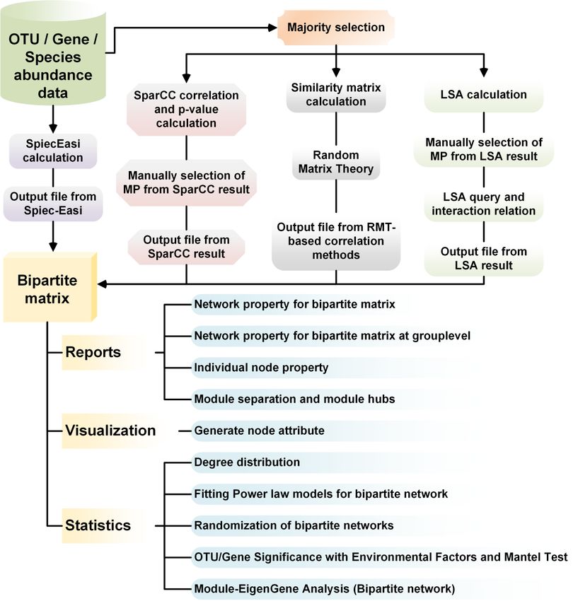
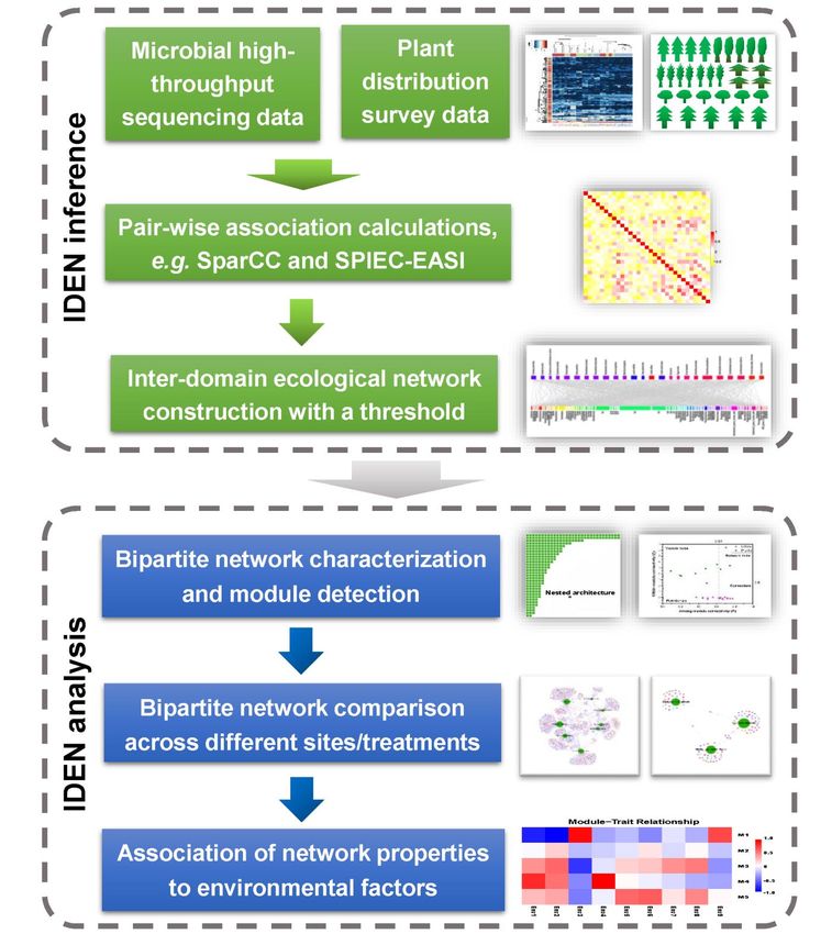
Steps of Inter-Domain Ecological Network Analysis

                        II
Workflow of IDENAP
IIIContent
To users.......................................................................................................................................... 1
A. Approaches to generate bipartite matrix .............................................................................. 2
1. SparCC ........................................................................................................................................................... 2
1.1 Majority selection ................................................................................................................................ 2
1.2 SparCC correlation and p-value calculation .................................................................................... 3
1.3 Manually selection of MP from SparCC result ................................................................................ 4
1.4 Output file from SparCC result ......................................................................................................... 5
2. eLSA ............................................................................................................................................................... 6
2.1 Majority selection ................................................................................................................................ 6
2.2 LSA calculation.................................................................................................................................... 7
2.3 Manually selection of MP from LSA result ...................................................................................... 9
2.4 LSA query and interaction relation ................................................................................................. 10
2.5 Output file from LSA result ............................................................................................................. 12
3. SPIEC-EASI ................................................................................................................................................ 13
3.1 SpiecEasi calculation ......................................................................................................................... 13
3.2 Output file from Spiec-Easi .............................................................................................................. 14
4. RMT-based method for Pearson/Spearman correlations ....................................................................... 15
4.1 Majority selection .............................................................................................................................. 15
4.2 Similarity matrix calculation ............................................................................................................ 15
4.3 Random Matrix Theory .................................................................................................................... 15
4.4 Output file from RMT-based correlation methods ........................................................................ 15
B. Bipartite network evaluations (Bipartite Network Analysis) ............................................ 16
1. Bipartite reports .......................................................................................................................................... 16
1.1 Network property for bipartite matrix ........................................................................................... 16
1.2 Network property for bipartite matrix at grouplevel .................................................................... 17
1.3 Individual node property .................................................................................................................. 18
1.4 Module separation and module hubs............................................................................................... 19
2. Bipartite visualization ................................................................................................................................. 19
2.1 Generate node attribute ........................................................................................................................ 19
3. Bipartite statistics ........................................................................................................................................ 20
3.1 Degree distribution ............................................................................................................................ 20
3.2 Fitting Power law models for bipartite network ............................................................................ 20
3.3 Randomization of bipartite networks .............................................................................................. 21
IV3.4 OTU/Gene Significance with Environmental Factors (Bipartite network) ................................. 23
3.5 Mantel Test ........................................................................................................................................ 24
3.6 Module-EigenGene Analysis (Bipartite network) .......................................................................... 26
C. Auxiliary tools in miscellaneous section .............................................................................. 27
1. Taxonomy summary of low level species for bipartite networks ............................................................ 27
2. Merge files .................................................................................................................................................... 28
3. Data location ................................................................................................................................................ 28
D. Operation tricks and common problem solutions .............................................................. 30
1. Upload .......................................................................................................................................................... 30
2. Basic operations in Galaxy ......................................................................................................................... 31
3. Dataset deletions .......................................................................................................................................... 32
4. Share historys to other users ...................................................................................................................... 32
If you have questions and is willing to make a contribution to this pipeline, please feel free to contact Prof. Ye
Deng (yedeng@rcees.ac.cn).
Pipeline maintainer: Kai Feng (kaifeng_st@rcees.ac.cn)
Please cite: Kai Feng, Yuguang Zhang, Zhili He, Daliang Ning, Ye Deng. Interdomain ecological networks
between plants and microbes. Molecular Ecology Resources. 2019,19 (6):1565-1567. doi:10.1111/1755-
0998.13081
VTo users
1. This pipeline is aimed to explore the inter-domain ecological networks, ignoring the
associations between intra-domain species.
2. Users are allowed to register account. Anonymous users are also allowed to operate in
this pipeline.
3. Since the limitation of server memory and the ability of association methods to handle
large dataset, we strongly recommend to reduce the No. of species/OTUs, i.e., not
exceed 2000 OTUs/species, otherwise the program will be disrupted or take a long time
(weeks to months).
4. Generally, we recommend SparCC and SPIEC-EASI to construct IDEN for beginners.
The other two methods, eLSA and RMT-based correlations, can also be used if you are
clear about these methods.
5. This pipeline is for research only, and please do not use for commercial activities.
6. Since our original goal of this pipeline is focusing on plant-microbe networks, we will
add a mark in each of names of species or OTUs to distinguish the two domain species,
i.e. “_P” to indicate plant and “_M” to indicate microbe. The two marks will be
removed during the construction of IDEN.
7. In order to reduce the potential errors, please do not include special characters in
species names and sample names, e.g. blank character, “-”, “#”, “$” and etc. And do
not use pure numbers in samples names or number started characters, i.e., “11”, or
“1A” and etc.
8. For new users, we provided a test dataset in the Shared library/Test data section.
1Instructions
A. Approaches to generate bipartite matrix
1. SparCC
https://bitbucket.org/yonatanf/sparcc/src/default/
Genomic survey data, such as those obtained from 16S rRNA gene sequencing, are subject to
underappreciated mathematical difficulties that can undermine standard data analysis techniques. We show that
these effects can lead to erroneous correlations among taxa within the human microbiome despite the statistical
significance of the associations. To overcome these difficulties, we developed SparCC; a novel procedure, tailored
to the properties of genomic survey data, that allow inference of correlations between genes or species. We use
SparCC to elucidate networks of interaction among microbial species living in or on the human body.
1.1 Majority selection
The majority is to filter the species or OTUs which were less detected among all samples. The integer of this
value is recommended as the 80% of the sample numbers.
Inputs:
2Parameters:
Input Parameter Value Note for rerun
1: OTU/Gene/Species abundance table for
Microbial data
PQG_otu_uclust_table_network.txt microbial community
Fill in the majority for
8 selected accordingly
first table
2: OTU/Gene/Species abundance table for plant
Plant table
PQG_plant_uclust_table_network.txt community
Fill in the majority for
6 selected accordingly
second table
Attention:
Do not use any symbols like ",","(",")","#","-" in your sample names
Do not start your sample name with numbers, e.g. "1A". Please rename it like "A1".
Outputs:
One tabular file contained filtered plants and microbes, named with their majorities.
1.2 SparCC correlation and p-value calculation
Inputs:
3Parameters:
Input Parameter Value Note for rerun
Input table for SparCC pseudo p-value 56: Filtered OTU/Gene/Species table
calculation Plant_6_microbe_8 with majority
Number of inference iteration to average over 20
Number of exclusion iterations to remove
10
strongly correlated pairs
Correlation strengh exclusion threshold 0.1
Number of shuffled times 100 Slow for more shuffle times
Compute one or two sided p-value Tow side p-values
Outputs:
Two tabular files: one is the correlation matrix, another is the p-value matrix.
1.3 Manually selection of MP from SparCC result
The step manually selects the pairwise interaction between microbe and plant from SparCC correlation
results. The selection is based on the marked symbols in the name like "_M" for microbe, "_P" for plant.
Inputs:
Outputs:
Two files only contain associations between plants and microbes.
41.4 Output file from SparCC result
Inputs:
Parameters:
Input Parameter Value Note for rerun
6: Selected SparCC correlation for each
SparCC correlation matrix Correlation matrix
pairwise
Threshold value to filter the SparCC Default value from
0.3
result SparCC
SparCC pseudo p value matrix after 7: Selected SparCC pseudo two_sided
P-value matrix
permutation side p-value
Filtering the SparCC result according to
yes Default
P value
Significance value 0.05
Visualization approach for this network
Cytoscape Cytoscape or Gephi
analysis
Title for the visualized output file - to visualization for SparCC result PQG_3 Put anything you want
remind you what the job was for P6M8 0.3 level 0.05 sig 100 perm to remember
5Outputs:
Nine output files (Cytoscape) for whole network matrix, positive sub-graph matrix and negative graph
matrix. For each matrix, there are a ‘sif’ file to importing into Cytoscape and an edge attribute file.
Six output files (Gephi) for whole network matrix, positive sub-graph matrix and negative sub-graph matrix.
For each matrix, there is a ‘csv’ file to importing into Gephi as edge file.
2. eLSA
The Local Similarity Analysis (LSA) technique is unique to capture the time-dependent associations
(possibly time-shifted) between microbes and between microbe and environmental factors (Ruan et al., 2006).
Significant LSA associations can be interpreted as a partially directed association network for further network-
based analysis. A similar approach called Local Trend Analysis (LTA) has also been developed for the state
change series, where a relative change threshold is applied to convert the original time series data into up-change,
no-change and down-change state series (Xia et al 2015). Many advanced network analysis tools (including ELSA)
have been analyzed in a benchmark paper published in the ISME Journal (Weiss et al. 2016). The more
introduction can be found in the home page (https://bitbucket.org/charade/elsa/wiki/Home).
2.1 Majority selection
The majority is to filter the species or OTUs which were less detected among all samples. The integer of this
value is recommended as the 80% of the sample numbers.
6Inputs:
Parameters:
Input Parameter Value Note for rerun
OTU/Gene/Species abundance table for
Microbial data 9: bac_16S_normal_format.txt
microbial community
Fill in the majority for
24 selected accordingly
first table
10: OTU/Gene/Species abundance table for plant
Plant table
plant_abundance_normal_format.txt community
Fill in the majority for
10 selected accordingly
second table
Attention:
Do not use any symbols like ",","(",")","#","-" in your sample names
Do not start your sample name with numbers, e.g. "1A". Please rename it like "A1".
Outputs:
One tabular file contained filtered plants and microbes, named with their majorities.
2.2 LSA calculation
This step is aimed to calculate the LS for each pairwise association.
Inputs:
7Parameters:
Input Parameter Value Note for rerun
Input table for lsa calculation 18: Plant_10_microbe_24
number of spots 4
number of replicates for each time spot 7
Integer and less than
maximum time delay 0
spot numbers
Method for p-value estimation Theoretical approximation
Permutation number 100 or
precision=0.01/permutation for p-value 100
estimation
Number of bootstraps for 95% confidence Bootstrap is not suitable
0
interval estimation for non-replicated data
Method to fill missing data fill up with zeros
Method to smmarize replicates data simple averaging
percentileZ normalization + robust
Method to normlize data estimates (with perm, mix and theo, and
must use this for theo and mix, default)
Qvalue calculation method R's qvalue package
8Outputs:
One tabular file contained local similarity score (LS) and other relevant scores.
Output explaination for each term
-X: factor name X
-Y: factor name Y
-LS: Local Similarity Score
-low/upCI: low or up 95% CI for LS
-Xs: align starts position in X
-Ys: align starts position in Y
-Len: align length
-Delay: calculated delay for align, Xs-Ys
-P,Q: p/q-value for LS
-PCC,Ppcc,Qpcc: Pearson's Correlation Coefficient, p/q-value for PCC
-SCC,Pscc,Qscc: Spearman's Correlation Coefficient, p/q-value for SCC
-SPCC,Pspcc,Qspcc,Dspcc: delay-Shifted Pearson's Correlation Coefficient, p/q-value, delay size for SPCC
-SSCC,Psscc,Qsscc,Dsscc: delay-Shifted Spearman's Correlation Coefficient, p/q-value, delay size for SSCC
2.3 Manually selection of MP from LSA result
The step manually selects the pairwise interaction between microbe and plant from LSA calculation
results. The selection is based on the marked symbols in the name like "_M" for microbe, "_P" for plant.
Inputs:
Outputs:
92.4 LSA query and interaction relation
This step is to filter LS according to your own criterion.
The matching pattern for LSA query should be filled correctly according to the recommended format.
[!]Key1[>,=,< =,==,!=]V1[|,&][!]Key2[>,=,Parameters:
Input Parameter Value Note for rerun
56: LSA for M-P pairwise
LSA pairwise calculation result
interaction
which coloum to select as filtration criterion Local Similarity Score 1st condition
what to do with the selected column of LSA table Greater or equal
Fill in the threshold value 0.8
Take opposite result No
The relation between this condition and the previous
Or 2nd condition
condition
which coloum to select as filtration criterion Local Similarity Score
what to do with the selected column of LSA table Less or equal
Fill in the threshold value -0.8
Take opposite result No
The relation between this condition and the previous
And 3rd condition
condition
which coloum to select as filtration criterion P-value for LS
what to do with the selected column of LSA table Less than
Fill in the threshold value 0.05
Take opposite result No
Outputs:
About the interaction type
- pu: positive undirected
- nu: negative undirected
- pdl: positive directed lead (X lead Y)
- ndl: negative directed lead (X lead Y)
- pdr: positive directed retard (X retard Y)
- ndr: negative directed retard (X retard Y)
112.5 Output file from LSA result
This step will generate three output files, including bipartite network matrix (or adjancency matrix),
visualization input (for Cytoscape or Gephi) and associated edge attributes if needed.
Inputs:
Parameters:
Input Parameter Value Note for rerun
Queried LSA pairwise 81: Queried LSA result
Visualization approach for this network analysis Gephi Cytoscape / Gephi
Interaction type Undirected Only for Gephi
Title for the output file - to remind you what the job Bipartite network matrix of
Put anything you want
was for, bipartite or adjancency LSA
Outputs:
Two output files (Gephi) for whole network matrix consisted of bipartite network matrix and import for
Gephi software.
12Three output files (Cytoscape) for whole network matrix consisted of bipartite network matrix, “sif” for
importing into Cytoscape and edge attribute file.
3. SPIEC-EASI
Sparse InversE Covariance estimation for Ecological Association and Statistical Inference. Please see more
in https://github.com/zdk123/SpiecEasi#cross-domain-interactions.
3.1 SpiecEasi calculation
Inputs:
13Parameters:
Input Parameter Value Note for rerun
Microbial data 1: PQG_otu_uclust_table_network.txt
Fill in the majority for first table 8
Inter-domain or intra-
Multiple domains T
domain
Plant table 2: PQG_plant_uclust_table_network.txt
Fill in the majority for second table 6
Estimation method glasso Glasso/MB selection
Number of penalties - somewhere
50
between 10-100 is usually good
Threshold for StARS criterion 0.05 Default
Minimum lambda 0.1 Default: 0.01
According to no. of
Number of subsamples for StARS 10
samples
Number of computational cores in
2 Not too large
parallel
Outputs:
SpiecEasi matrix: A matrix for inverse covariance, used to infer associations.
SpiecEasi report: A report for SPIEC-EASI processing.
Filtered matrix with majority: OTU/Gene/Species table after majority selection
3.2 Output file from Spiec-Easi
This step will generate three output files, including bipartite network matrix, visualization input (for
Cytoscape or Gephi) and associated edge attributes if needed.
Inputs:
14Parameters:
Input Parameter Value Note for rerun
SpiecEasi matrix 134: SpiecEasi matrix
Generate bipartite network or single-mode network Bipartite network Bipartite network or
single-mode
Visualization approach for this network analysis Cytoscape Cytoscape/Gephi
Title for the visualized output file visualization for Spiec-Easi Put anything you want
Outputs:
Nine output files (Cytoscape) for whole network matrix, positive sub-graph matrix and negative graph
matrix. For each matrix, there are a ‘sif’ file to importing into Cytoscape and an edge attribute file.
Six output files (Gephi) for whole network matrix, positive sub-graph matrix and negative sub-graph matrix.
For each matrix, there is a ‘csv’ file to importing into Gephi as edge file.
4. RMT-based method for Pearson/Spearman correlations
Generate bipartite networks using Pearson/Spearman correlations with RMT-based cutoff. (Coming soon)
4.1 Majority selection
4.2 Similarity matrix calculation
4.3 Random Matrix Theory
4.4 Output file from RMT-based correlation methods
15B. Bipartite network evaluations (Bipartite Network Analysis)
All statistics analysis methods were based on bipartite network matrix. The simple format for this matrix
is illustrated as following:
1. Bipartite reports
1.1 Network property for bipartite matrix
Inputs:
Parameters:
Weighted or Unweighted: unweighted
Weighted NODF: an index to indicate nestedness.
Outputs:
161.2 Network property for bipartite matrix at grouplevel
This step calculates the network properties for the two groups of species shown in the bipartite network
matrix, e.g. higher lever for column species (plants in this pipeline), and lower level for row species (microbial
data in this pipeline).
Inputs:
Parameters:
Weighted or Unweighted: unweighted
17Outputs:
1.3 Individual node property
Inputs:
Outputs:
181.4 Module separation and module hubs
There are four methods provided in this pipeline for modularization: greedy modularity optimization, short
random walks and leading eigenvector of community matrix. Besides, the Z-P result can provide information of
module hubs.
Inputs:
Parameters:
Modularity method: Greedy modularity optimization / Short random walks / Leading eigenvector of the
community matrix / Simulated annealing (slow). Select according to previous choice.
Outputs:
2. Bipartite visualization
2.1 Generate node attribute
Inputs:
19Parameters options:
Visualization software approach: Cytoscape / Gephi
Outputs:
A tabular file for Cytoscape or a csv file for Gephi.
3. Bipartite statistics
3.1 Degree distribution
Fits functions to cumulative degree distributions of both trophic levels of a network. This program is
mainly for cumulative distribution.
Inputs:
Outputs:
3.2 Fitting Power law models for bipartite network
Fitting Power law models for bipartite network regular power law, log power law, exponential law and
truncated power law. This fitting is mainly to use node connectivity or node degree as response.
Inputs:
20Outputs:
3.3 Randomization of bipartite networks
Inputs:
Parameter options:
Methods:
Rewiring links keeping node degree constant: rewiring the links between the randomly selected two
links.
Shuffle.web: It implements a method where matrix is first filled honouring row and column totals, but
with integers that may be larger than one. Then the method inspects random 2x2 matrices and
performs a quasiswap on them. It is similar to ordinary swap, but it also can reduce numbers above
one to ones maintaining marginal totals.
21 Mgen: This is a generic function to build null models for mutualistic networks, used by Vázquez et al.
(2009). It is general in the sense that it allows any type of probability matrix to be used for
constructing the simulated matrices. It does not, however, constrain rown and column totals, nor does
it constrain connectance.
No. of random matrix: 100
Weighted or unweighted: Weighted. Average according to their number of interactions or treat nodes
equally
Weighted NODF: No
Modularity separation method selection: Greedy modularity optimization / Short random walks /
Leading eigenvector of the community matrix / Simulated annealing (slow). Select according to previous
choice.
Outputs:
223.4 OTU/Gene Significance with Environmental Factors (Bipartite network)
The output of this program can be used for significance test using Mantel test for further analysis.
Inputs:
Parameter options:
Filtered matrix with microbes and plants
Bipartite network matrix
Environmental factors
Correlation method: Pearson Correlation Coefficient / Spearman Correlation Coefficient
Standardization method: standardize environmental data only (scale each factor to zero mean and
unit variance) or other choice
Missing values: ignore (only use paired values)
Outputs:
233.5 Mantel Test
For mantel test:
Inputs:
Parameter options:
Select the corresponding files according to the labels shown in the pipeline.
Mantel type: Mantel test or Partial mantel test
Annotation file: (Optional)
Upload your annotation file related to OTU/Gene names: No / Yes (if you have uploaded)
Outputs:
24For partial mantel test:
Inputs:
Parameter options:
Select the corresponding files according to the labels shown in the pipeline.
Mantel type: Mantel test or Partial mantel test
Annotation file: (Optional)
Upload your annotation file related to OTU/Gene names: No / Yes (if you have uploaded)
Outputs:
253.6 Module-EigenGene Analysis (Bipartite network)
Inputs:
Parameter options:
Select the corresponding files according to the labels shown in the pipeline.
Outputs:
26C. Auxiliary tools in miscellaneous section
1. Taxonomy summary of low level species for bipartite networks
This tool is mainly used to assign different OTUs or species into higher taxonomic level, e.g. phylum and
genus, and then generate sub-graph matrix for each group at the specific level.
Inputs:
Parameters:
Bipartite network matrix: matrix of bipartite graph
Sample list: Not useful at this stage
OTU classification result from RDP classifier: OTU/Gene/Species classification file
Count species richness or count species abundance: Species abundance / Species richness
Summary result type for each sample: Numbers / Percentage
Select which taxonomy level to calculate result: Phylum (select from classification file)
27No. of species showing in the plot: 0
Output:
One file contains the bipartite network matrix at the specific taxonomic level and another plot is the summary
for this level.
After download the zipped file to local directory, you need to unzip this file twice. For the first step of
unzipping process, you can easily unzip it. For the second step of unzipping process, you need to rename the
extension file type to “.zip” or “.gz” and thereafter you could to unzip this file. After the two steps of unzipping,
you can see the separated txt files.
2. Merge files
This tool is mainly used to merge multiple files into one file.
Input:
Output:
Succession (If you put another name in the “rename the merged file”, it will show what you have fill in.)
3. Data location
This tool is mainly used to find the data location for certain dataset in the server. The data location is
helpful to find the dataset for Galaxy administrators when you have problems.
Input:
28Output:
file_location.txt
29D. Operation tricks and common problem solutions
1. Upload
Upload the all the OTU tables or environmental variable datasets to selected history.
Upload button(multiple files are available)
Required files:
You can find following test data from the “shared library/test data” directory and import these three files
there.
302. Basic operations in Galaxy
Please remember to choose “choose permanently” if you want to erase your history permanently, otherwise it
will store into a temporary place and your quota will not decrease. See the below introduction for how to find
temporarily deleted history.
Copy datasets:
313. Dataset deletions
Select “saved history” and further choose “Advanced Search” button:
Choose “all” button to show all history that you have created in your account. And select the deleted history to
further erase or retrieve.
4. Share historys to other users
Select “share or publish” of a certain history, then fill in the individual users:
32You can also read