Social In uence in the U. S. House of Representatives, 1801-1861
←
→
Page content transcription
If your browser does not render page correctly, please read the page content below
Social Influence in the
              U. S. House of Representatives, 1801-1861
                           William Minozzi∗ Gregory A. Caldeira∗
                                               May 16, 2015

                                                   Abstract

       Legislatures are plainly social places. Yet, there is at best mixed evidence of social in-
       fluence in this setting. We argue that the main reason for the lack of consensus is that,
       as difficult as it is to detect evidence of social influence in general, it is even more dif-
       ficult in modern legislatures, in which there are many potential ways that legislators
       can affect one another. Thus, we focus on the U.S. House of Representatives before
       the Civil War, a time during which most members lived together in boardinghouses,
       in small groups, within isolated, concentrated conditions, under weak political insti-
       tutions, and subject to strong norms to socialize. We have collected the universe of
       extant evidence on residences of members of Congress for the period between 1801
       and 1861. Using these data, we find that co-residence both predicts and causes in-
       creases in voting agreement. Perhaps most compellingly, we leverage the occurrence
       of occasions when a legislator died in office to identify the effects of their (exogenous)
       removal from the social network on the ideological voting patterns of their erstwhile
       co-residents. We find that these deaths caused increases in the ideological distance
       between the surviving and deceased.

   ∗
     Ohio State University. Prepared for the Congress & History Conference, Vanderbilt University, May 22-23,
2015. We thank Skyler Cranmer and Michael Neblo for helpful conversations, and Jakob Miller for valuable research
assistance. Email: william.minozzi@gmail.com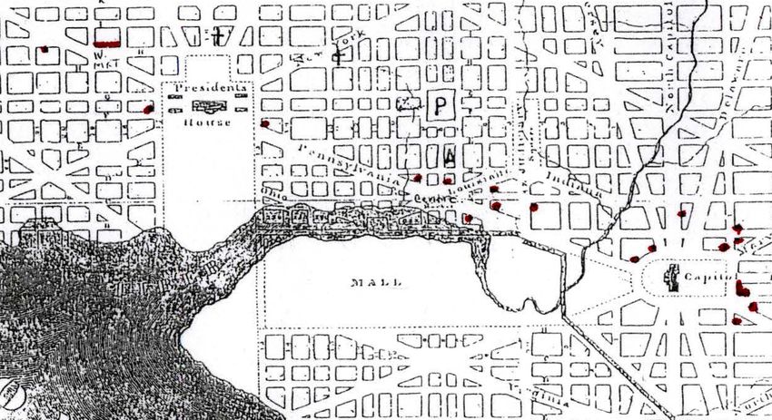
Introduction
Legislatures are social places. Some of the classic works in legislative politics spotlight the role of
social ties in cue-taking and voting (Matthews and Stimson 1975; Kingdon 1989); and more recent
work has emphasized the role of collaboration in co-sponsorship (Fowler 2005, 2006), committee
work (Porter et al. 2005, 2007; Ringe, Victor, and Gross 2013), and physical proximity (Masket
2008; Liu and Srivastava 2015) as salient social components of legislatures. Of primary interest is
the role of social influence (Friedkin 1998): the idea that one actor’s behavior can affect another’s
preferences, beliefs, and actions.
   Despite the social aspect of legislation, the workhorse model of legislative behavior—the spa-
tial model—excludes social influence among members. Amendments to this model are typically
strategic, rather than more generally social. Moreover, there is at best mixed evidence of social
influence in legislatures, with the best identified design finding no evidence of social influence
(Rogowski and Sinclair 2012). Because social influence is difficult to credibly detect in general
(e.g., Shalizi and Thomas 2011) and the evidence of social influence is so far mixed, social theories
of legislative politics remain peripheral.
   One reason for the paucity of evidence of social influence in legislatures is that there are
so many possible avenues on which one legislator may affect another. Even if one legislator is
heavily influenced, say, by a roommate, she may be one of only a few for whom “roommate” is
the most important vector. Another legislator may take cues from his caucus. A third may take
direction from her staff, who are in turn influenced by friends from the staff in an adjacent office.
Looking for credible evidence of social influence along a single vector in a modern legislature is
a bit like trying to identify which pellet from a shotgun blast was deadly.
   The modern legislature is the wrong place to look for perceptible evidence of social influence
in legislative behavior. A better prospect is the era of boardinghouses—Washington DC before
the Civil War—a place and a time when legislators were isolated and concentrated, governing
under relatively weak political institutions, but living together in dense social networks rife with

                                                  1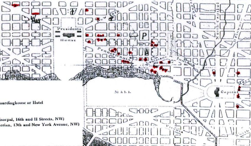
political discussion. Although we offer no expectations about whether the degree of social influ-
ence has changed over time, we do expect that it was much more concentrated, and thus more
easily detectable, in this setting.
   We make several contributions. First, we collect the universe of extant evidence on residences
of members of Congress for the period between 1800, when the seat of the United States govern-
ment moved to Washington, and the Civil War. Second, we use these data to present patterns of
residential life in this period, finding, for example, ramifications of the collapses of the early party
systems. Third, we conduct session-by-session and panel analyses of legislator dyads, focusing on
the relationship between co-residence and voting agreement. Here, we find that co-residence both
predicts and causes increases in agreement; these findings are statistically significant, though of
(plausibly) small size. Fourth, and finally, we leverage information on legislators who died in
office to identify the effects of their deaths on the ideological voting patterns of their erstwhile
co-residents. We find that these deaths caused increases in the ideological distance between the
surviving and deceased.
   The remainder of the paper is structured as follows. First, we discuss the literature on social
influence in legislative politics. Next, we argue that residential networks before the Civil War
are an ideal place to find evidence of social influence. Then we present our data, after which
we discuss patterns in residential life during the pre-Civil War period. Subsequently, we present
three analyses of co-residence and voting: a session-by-session analysis, a panel study, and a
study based on legislators’ deaths. We then conclude.

Social Influence in Legislative Behavior
The workhorse model of legislative behavior, the spatial model, features a set of inert, atomic
legislators with fixed and inviolable preferences. This model of legislative behavior postulates
that, for a legislator to cast her vote, she needs to know only three pieces of information: the
locations of her ideal point, of the status quo policy, and of the alternative. Nearly universal is
the spatial model as an explanation of legislative behavior. Based on the perspicuity and power

                                                   2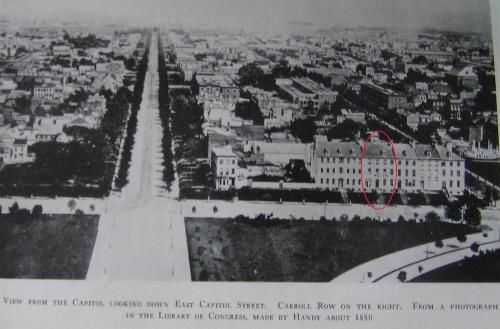
of the spatial model, a prominent line of criticism even calls into question the causal role of
party affiliation on congressional behavior (Krehbiel 1993, 2000). Fixes or amendments to the
model in response to anomalous results generally involve strategically transferring utility (e.g.,
distributive goods or money)—not to influence preferences but to compensate for the casting of
otherwise undesirable votes (e.g., Cox and McCubbins 1993, 2005; Jenkins and Monroe 2012).
   Even though legislating is plainly a social act, the parsimony of the spatial is purchased at
the cost of most conventional notions of social behavior. The critical omission from the spatial
model is social influence, the idea that a person’s preferences may be affected endogenously by
the behavior of another (e.g., Friedkin 1998). Even in an institution as structured and constrained
as the Congress, social influence might nonetheless be pervasive because of the sheer difficulty of
the legislator’s job (Kingdon 1989; Matthews and Stimson 1975). In complex, collective decision-
making institutions, individual actors must deal with risk, uncertainty, too much and too little
information, inadequate time and resources, and so forth. It is natural to expect social influence
to characterize individual legislators’ decisions.
   We take social influence to be endogenous change in a person’s political behavior as a re-
sult of another person’s behavior. Such influence can manifest itself in either convergence or
divergence of attitudes and beliefs. There are many different theoretical formulations of social
influence in networks. Its constitutive mechanisms include, but are not limited to, strategic infor-
mation transmission (e.g., Galeotti, Ghiglino, and Squintani 2013), cue-taking (e.g., Matthews and
Stimson 1975), and norm reinforcement (e.g., Liu and Srivastava 2015), as well as more general-
ized dynamics (e.g., Siegel 2009). Regardless of the precise mechanism, physical proximity (e.g.,
Masket 2008) and propinquity (e.g., Lazer et al. 2010) enhance these mechanisms, whereas salient
differences can cause them to backfire and become polarizing (e.g., Baldassarri and Bearman 2007;
Ringe, Victor, and Gross 2013; Liu and Srivastava 2015).
   Despite the dominance of the spatial model, there is a distinct lineage of political scientists
who study social influence, and networks more generally, in legislatures. Routt (1938), in his study
of the Illinois Senate, describes legislators as first and foremost specialists in human relations for

                                                     3
whom the technique of interpersonal influence and persuasion is paramount. Kingdon (1989) and
Matthews and Stimson (1975) highlight and demonstrate the importance of cue-taking in voting
in Congress. Caldeira and Patterson (1987) and Caldeira, Clark, and Patterson (1993) study the
role of propinquity in the formation of friendship and respect in state legislatures. Ringe, Victor,
and Gross (2013), in their study of a committee in the European Parliament, and Liu and Srivastava
(2015), in their study of the recent U. S. Senate, both emphasize the polarization that can occur
when legislators with disparate social identities come into close contact with each other. And
this list remains an incomplete inventory of studies of social networks in legislative politics.
In light of the apparent abundance of scholarship on social networks in legislatures, it is at
first puzzling that the spatial model of legislative politics has not given way to a more social
theory. The primary reason seems to be that detecting social influence in a body as diverse and
complex as Congress is remarkably difficult to do in a credible fashion. There are several reasons
for this difficulty. Principally, there is the generic threat of confounding (e.g., Manski 1993; Shalizi
and Thomas 2011). For example, suppose two legislators have some social tie through which one
is theorized to influence the other’s voting behavior. Evidence of correlation between their votes
may indeed indicate social influence, but it could also result from homophily, in which people
choose to socialize because of their initially harmonious views, or common exposure, in which
both are influenced by a third, unmeasured force. Indeed, there is an important similarity between
the diagnosis of confounding in social networks and Krehbiel’s (1993) argument that the causal
effects of party and ideology are inextricably entangled. Just as Krehbiel recommends relying
on the more parsimonious (and partyless) preference-based theory, scholars of legislative politics
might believe that, in the absence of credible, causally-identified evidence of social influence, the
spatial model, perhaps now augmented by strategy and parties, is preferable.
A second reason scholars of legislative politics may prefer the spatial model is that the most
credible and recent studies of social influence have yielded mixed results. Consider the contrariety
of evidence on whether physical proximity affects legislative voting. First, Masket (2008) takes
advantage of desk-mates in the California Assembly’s chamber and identifies significant evidence
4of social influence. Second, Rogowski and Sinclair (2012) use the office lottery for congressional
offices to identify effects of office proximity on voting. They find null effects. Finally, Liu and
Srivastava (2015) conduct a longitudinal network study and find evidence that U. S. senators
from different parties display decreasing voting agreement as the distance between the desks
diminishes. Of these studies Rogowski and Sinclair’s (2012) is arguably the most compelling, as
it is the only one that leverages a genuine source of exogeneity; the other two attempt to isolate
the effects of endogenous, and perhaps confounded, variables. At the least, with disagreement
in the empirical literature, scholars may simply not be convinced that social influence is worth
complicating their workhorse theory.
We contend that there is an alternative reason these mixed empirical findings have emerged,
and that it is consonant with pervasive social influence in legislatures. Modern legislatures should
be exceptionally difficult places to study social influence—even if we expect it to be ubiquitous.
Members of Congress are exposed to extremely varied sources of social influence, and social sci-
entists in search of causally identified, measurable, and statistically significant effects must sort
out: information; a multitude of competing, conflicting cues; the effects and sources of strong
parties; strong leadership in the House; intense, often diverse constituencies; financial contribu-
tors; round-the-clock mass media; and lobbyists in hordes. Moreover, legislators may well want
to conceal the effects of many of these sources from their constituents. Studies of social influ-
ence in legislatures inevitably focus on a single vector—e.g., office of desk proximity, committee
co-memberships, etc. Social influence might be pervasive but undetectable if different legislators
are influenced through different vectors. One legislator may be most influenced by a neighbor
on the chamber floor; another, by a member of a similar religious faith; and a third, by fellow
legislators lobbying for allied interest groups. For the modern Congress, the incredible difficulty
of collecting information on and of measuring and assessing the impact of social interaction is
layered on the equally difficult problem of teasing out the impact of the variety forces we can
(and cannot) measure. There is no one single vector of social influence that is the most obvious
one on which to focus.
5Thus, we hearken back to a period in which the vectors of social influence in Congress were
less varied and more intensely focused: to boardinghouse life in pre-Civil War Washington, DC.
In the next section we describe social life in these boardinghouses and contend that Washington
DC in its infancy is a promising site to measure and assess social influence in a legislature.
Social Life in Washington before the Civil War
Social life in Washington before the Civil War was intense and inward-focused. As a result, resi-
dential life during this period is a particularly promising vector of social influence to investigate.
Drawing heavily on Green (1962), Young (1966), Earman (1992, 2000, 2005), and Shelden (2011,
2013), we develop four reasons for this conclusion. First, members were physically isolated from
the rest of the country. Once in Washington, members had to reside there for months at a time.
Second, members were residentially and socially concentrated. Legislators who lived together
were likely to encounter each other frequently, especially over meals, on errands, and travel-
ing to and from the Capitol. During these activities, politics was bound to be the preeminent
topic of conversation. Third, members faced few of the institutional constraints present the mod-
ern Congress—e.g., strong parties; the mass media; strong, specialized committees; and lobbying
groups. Fourth, and finally, members were virtually compelled to interact with each other by the
strict social expectations of the era for men of their class, an established ritual of social rounds
which forced social contact among and between virtually every member of the federal establish-
ment. Thus, we propose that this era should be a particularly promising place to look for signs of
social influence. Put another way, if we cannot find it here, we are surely unlikely to find it later
in the modern Congress.
The Isolation of Washington
The primitive state of transportation and roads meant that most representatives had to travel for
weeks to reach home. Serving in Congress meant social isolation from everything familiar and
comforting—families, friends, and associates (Riley 2014; Zagarri 2013).
Especially during the early part of the 19th century, the grand City of Washington remained
6an imaginary vision on L’Enfant’s original design, in Dickens’ phrase, “a City of Magnificent
Intentions.” The Federal District, and the government within it, rose from an unlikely site in a
swamp, in which in 1800 there were only 400 useable buildings in the 10 miles squared, most of
them rudimentary and not habitable by the likes of congressmen.1 Well into the 19th century,
most observers considered life in Washington to be primitive by the standards of the main Amer-
ican cities. And, as if to exacerbate the sense of isolation and force social intercourse among
living mates, there was little to do in Washington—few amenities; a sparse population composed
of plantation notables not open to outsiders, tradesmen and laborers, and slaves and free blacks;
and limited choices for lodging. Moreover, postal service was slow, a letter taking a week or more
to move from Washington DC to New England and even longer to the westernmost part of the
country. So, communication between members and home was sporadic, slow, and uncertain, no
doubt making representatives feel all the more alone.
The rough geography of the District, imprecise street markings and addresses, and long dis-
tances between and among clusters of residences and gathering places meant that going from
one part of the City to another was a trial. Some representatives lived in Georgetown, the most
developed city in the District, but this meant a carriage ride of an hour or so both ways. Perhaps
the most significant divide in the first part of the century was the placement of the executive
branch and Congress at opposite ends of Pennsylvania Avenue. In Jefferson’s design of the seat
of government, the White House and Capitol would have resided in close proximity, much like
the arrangements in New York and Philadelphia, where members of the executive branch and
Congress were intermixed. Of course, L’Enfant’s design prevailed and the executive and legisla-
1 On arriving in the vestigial federal city, Treasury Secretary Oliver Woolcott wrote to his wife: “I have made every
exertion to secure good lodgings near the office, but shall be compelled to take them at the distance of more than half
a mile. There are, in fact, but a few houses at any one place, and most of them small miserable huts, which present
an awful contrast to the public buildings.—The people are poor, and, as far as I can judge, they live like fishes, by
eating each other. All the ground for several miles around the city being, in the opinion of the people, too valuable
to be cultivated, remains unfenced. There are but few enclosures, even for gardens, and those are in bad order. You
may look in almost any direction, over an extent of ground nearly as large as the city of New York, without seeing
a fence or any object except brick-kilns and temporary huts for laborers. Greenleaf’s Point presents the appearance
of a considerable town which had been destroyed by some unusual calamity. There are (at Greenleaf’s Point) fifty or
sixty spacious houses, five or six of which are occupied by negroes and vagrants, and a few more by decent working
people; but there are no fences, gardens, nor the least appearance of business.” Letter, July 4, 1800.
7ture clustered at what were then substantial distances.
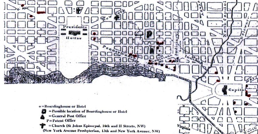
Figure 1 collects three maps drawn from Young (1966) and Earman (1992), which provide the
best current approximation of the location of boardinghouses and residences during three con-
gresses ranging from 1807 through 1830. For many of the boardinghouses, and even of the hotels,
it is difficult and sometimes impossible to pin down exact locations, so these maps underestimate
the number and probably the dispersion of residences; but they give us a general idea, especially
when viewed in sequence. The first covers the 10th Congress (1807-1809). Note the isolated con-
centrations around Capitol Hill, near the White House, and several in Georgetown; and that there
was not much in the middle of the main thoroughfare, Pennsylvania Avenue. In the second figure,
for the 16th Congress (1819-1821), we see, in general, more residential buildings, more around the
Capitol, more around the President’s House, and now several now in the middle of Pennsylvania,
such that we are beginning to see a connection between the White House and Capitol. Finally, in
the third, for the 21st Congress (1829-1831), a substantial set of buildings lines Pennsylvania and
links the two branches of government.
Concentration in Social Life
Scarcity of places to live and eat meant that members had no choice but to live with other mem-
bers. Residential options were limited to three principal alternatives: hotels, private residences,
and boardinghouses. Hotels in the modern sense did not exist in the first years of the 19th century.
One early attempt to create a large and modern hotel in Washington failed for lack of financing
(Bryan 1904). Early on buildings denominated as “hotels” were actually large houses or series of
connected buildings. Gradually and only later did modern hotels come onto the being and thrive.
Social life in hotels for members of Congress of course included opportunities to encounter many
other legislators, but co-residents of hotels were not guaranteed to interact.
Wealthier residents sometimes sought private residences, either renting them or purchasing
them outright. For example, several members of Congress purchased or rented residences on
President’s Square, just north of the White House, near wealthy Washingtonians like William
8Figure 1: Maps of Boardinghouse Locations during the 10th, 16th and 21st Congresses
9Corcoran. A somewhat less secluded option was boarding in private residences not advertised
to the public. For example, John Quincy Adams took in boarders and long-term guests at times
throughout his long residency in Washington. Private residences by definition isolated a member
unless he was joined by others. Members of Congress who lived in them would have had the
opposite experience from that of hotel dwellers, with limited interaction following from their
social seclusion.
By far the most common residential selection was the boardinghouse. Boardinghouses varied
greatly in size, expense, quality of meals, and the social composition of boarders. Representatives
might be forced to share rooms, either because of cost or lack of options. Perforce representatives
shared meals with co-residents, whether other members, military officers, professionals, or trav-
elers of various occupations, sometimes rough personages. Some boardinghouses had staying
power and developed a distinct political character; most lasted for brief periods, sold and re-sold,
some going bankrupt, disappearing only to reappear under the name of a different proprietor. At
times the proprietors themselves moved around, often taking the name of their boardinghouse
with them.
Carroll Row featured some of the most famous of Washington’s boardinghouses (see Figure 2).
These mid- and late-19th century photographs show Carroll Row, sometimes called Six Buildings
or Duff Green’s Row, on First Street between East Capitol and A Streets, SE. They have since
been torn down to make way for the Library of Congress. Daniel Carroll, who was one of the
great property owners of the District, built these row houses as well as fifteen or twenty others
on speculation in the years before the government relocated. The Supreme Court resided and
deliberated there for parts of the period between 1815 and 1835; and, during the period after the
1814 fire, it held its sessions there. Later, the eastern-most house became Mrs. Sprigg’s, which
housed mostly a diverse set of Whigs and became a haven for abolitionists, including Joshua
Giddings of Ohio, one of its most ardent advocates in the House, and his allies William Slade of
Vermont, and Seth Gates of New York; and, for a time, Theodore Dwight Weld and Joshua Leavitt,
who were publicists for abolition. Mrs. Sprigg, although a former slave owner, was known as a
10Figure 2: Four Views of Carroll Row Boardinghouses
11quiet abettor of the underground railroad (Winkle 2013). In Abraham Lincoln’s single term in
Congress he lived at Mrs. Sprigg’s, sometimes joined by his family. Residing at Mrs. Sprigg’s
placed him in the midst of abolitionists, and in close proximity to slave pens and trading, and
undoubtedly helped him to sharpen his ideas about slavery. It was but 50-100 feet from the park
south of the Capitol, within a short walk of the Capitol, and was a prime location for members of
Congress as well as many others. Carroll Row became a particularly prime location in the period
after the British burned the Capitol and again during the Civil War, when the federal government
leased some of its buildings.
Mrs. C. A. Pittman’s boardinghouse, located on the west side of 3rd Street between Pennsyl-
vania Avenue and C Street, was another mainstay of the late 1830s and early 1840s and housed a
long list of members. Its denizens tended to be Democrats or conservative Whigs and at various
times James Buchanan, Franklin Pierce, and Millard Fillmore resided there. Unlike other propri-
etors, Mrs. Pittman served no alcohol. Perhaps for that reason, Franklin Pierce and his wife stayed
there in the session 1837; in the previous session, Pierce had suffered grievously the death of their
child and apparently treated himself with great amounts of alcohol. One resident commented:
“There is not a wine drinker among us. Even Franklin Pierce has left off.” In the close quarters of
a boardinghouse, co-residents quickly learned each otherfis strengths and weaknesses.
We are fortunate that Representative Amasa J. Parker, a Democrat from New York, included a
drawing of this boardinghouse in one of many letters to his wife (December 31, 1837). Residents
and messmates here included Zadock Pratt (D, NY), Senator Samuel Prentiss (Whig, VT) and wife,
Hugh Anderson (D, ME), John H. Prentiss (D, NY), Andrew Buchanan (D, PA), Senator Nehemia
Knight (Whig, RI) and wife, Millard Fillmore (W, NY) and wife, Heman Allen (W, VT), John Fair-
field (D, ME), Samuel Birdsall (D, NY) and wife, Robert McClelland (D, NY), Albert White (Whig,
Indiana), Parker, and Hopkins Holsey (D, Georgia). Several features of this diagram stand out.
First, the dining room and parlor for members of Congress and their spouses are separate from
those for other boarders, which is probably one of the reasons the term “mess” came into usage.
This arrangement permitted members to conduct political business over meals and to meet with
12guests in relative privacy; the large, oval table made for conviviality. Second, several wives were
in residence, reflecting a growing trend. Third, Mrs. Pittman’s, like many boardinghouses, was
composed of connected buildings. Parker here shows his room on the first floor in the adjacent
building, around which was a yard.
Expectations of privacy were quite different in the 19th century, and it was not unusual even
for wealthy people to have friends, family, or associates live with them for extended periods
of time. Until the 19th century, taverns, not boardinghouses or hotels, were the equivalents
of today’s hotels; and taverns were simply houses with a public room for drinking and eating
and bedrooms upstairs. Customers of every social class simply showed up and took whatever
accommodation happened to be available. A gentleman might find himself shoulder to shoulder
with a member of a “lower order” at the dinner table and then body to body in a bed upstairs. Thus,
boardinghouses in Washington catering to members of Congress were a major improvement.
Once members and executive officials started owning houses, they might invite another member,
or a local might invite a member, even with family, to board with them for a time. Over time,
more and more members brought wives and families, making life much more comfortable and
civilized, but this did not happened on a widespread basis well into the ante-Bellum era.
Members’ lack of offices reinforced the lack of privacy and forced even more social interac-
tions with other members. Not until the latter part of the 19th century did senators have offices,
with the House following in 1913. Until then, members worked at their desks in the Senate and
House chambers. Thus, the location of a desk was critical, in the status it signified, the affinities
of those seated at adjacent desks, and its convenience to the front of the chamber. In a typical
day, a member rose in his boardinghouse, took a collegial meal, and retired to cope with a first
delivery of mail; at 10 a.m. headed over to his desk at the Capitol to take up more mail and docu-
ments delivered by messengers and to chat with colleagues, and spent the remainder of the day
in the Chamber once a session began; retired to a 4 pm dinner, again among co-residents of his
boardinghouse; and in the evening often went with his colleagues to a reception or to pay calls.
This was not a place for introverts.
13Figure 3: A Map of Seating at Mrs. Pittman’s, Outlined in Rep. Amasa Parker’s Letter to his Wife,
December 31, 1837, 25th Congress.
14Weak Political Institutions
Compared to today’s members, who must deal with a congeries of lobbyists, financiers, executive
officials, active constituents, and a twenty-four mass media, 19th century members faced a rel-
atively simple political environment made up of colleagues; sporadic visits from constituents; a
steady flow of mail from constituents, mostly asking for intercession with a federal department;
and contacts with executive officials, most of them directed at the executive rather than the other
way around.
Political parties, of course, were not solidly entrenched as political institutions and as leaders
and sources of influence until the 1830s; early on partisan labels and attachments were not as
meaningful and persistent as they later became, and sectional conflict often counteracted budding
partisanship as the composition of the congressional agenda changed.
Organized interests did not exist, even in vestigial state, until after the Civil War. Lobbying
in early congresses consisted mainly of constituents seeking pensions, public lands, patents, or
other benefits from the federal government, with members serving as conduits to the relevant
executive department. So, for example, a member might receive a letter or visit from a constituent
and consequently stop in to check on the status of a patent down the street in the Patent Office
or walk a bit further to chat with a clerk in the Land Office, to establish the status of land parcel.
To the extent it occurred, organized lobbying came in the form of petitions calling for some
legislative action and signed by groups of constituents from his district, which the member then
introduced in the Chamber.
Presidents and cabinet members generally did not engage in lobbying Congress, although
there was much more contact from the latter than from the former. To the extent presidents
lobbied at all, they did it informally, over dinners and on social occasions, always in or around
the White House. Presidents by precedent did not call on others and owed no one a visit, so social
interaction had to occur on his turf. Jefferson was unique and the most ambitious in his pursuit
of organized congressional action. He orchestrated carefully planned, regular dinners several
15times a week during sessions from the first to the end of his last Congress (Scofield 2006).2 The
format of these dinners was informal, although food and drink were elegant and plentiful. To
color the tone of the meal, Jefferson prohibited explicit discussion of current political issues and
observation of court manners and diplomatic status, and he made a point of mixing men and
woman, members of opposing parties, and people from the community. The purpose was to have
members experience his charm, create mutual sympathy, and to disarm them in future maneuvers.
Political talk then took place in post-prandial groups amid cigars and alcohol. These dinners are
but one example of the extensive contact social, explicitly non-political activity across branches
of government (Allgor 2002; Earman 2005), contrary to the claims Young and others have made
about the dullness of social life and the social separation between Congress and the executive
during the pre-Civil War period
Standing congressional committees in a recognizable form did not come full-blown into be-
ing until the 1820s (Gamm and Shepsle 1989; Jenkins 1998) and even then committees were not
institutionalized, committee “property rights” had partially crystallized, chairs did not exercise
as much authority, structure was relatively simple, subcommittees did not exist on a permanent
basis, and seniority had not taken hold. Thus, individual members then did not face as clear a
committee signal on legislation or as committee members feel the constraints of decisions made
within those smaller groups.
Instability in membership undermined the impact of personal connections and institutional
pressure. Politicians did not view Congress a career until well after the Civil War (Polsby 1968);
campaigns were highly competitive, electoral tides volatile, turnover sometimes dramatic, and,
consistent with a norm of “rotation in office,” most members would serve one or two terms and
retire, perhaps return some years later; and few development long-term seniority (Kernell 1977;
Struble 1979-1980).
Finally, newspapers were controlled by party entrepreneurs and generated competing, par-
2 He left manuscripts in which he had listed all members of Congress, of both houses; listed guests at each occasion;
noted who showed up or declined; and made checks on names for numbers of dinners attended as the year passed
(Scofield 2006).
16tisan streams of information (Pasley 2002; Carson and Hood III 2014) and therefore did not pro-
vide the kind of information constituents could use to make an independent evaluation of their
representatives (but see Carson and Hood III 2014; Bianco, Spence, and Wilkerson 1996). Mem-
bers themselves produced much of the fodder for newspapers by using their franking privilege
to distribute speeches and other documents. Thus, members had great latitude so long as they
maintained strong ties to their respective parties, in which newspapers were a crucial cog.
Strict Social Norms
In contrast to the relatively weak political institutions of the period, social institutions were elab-
orate and well-developed and forced and reinforced social interaction. President Washington
immediately took pains to articulate a formal set of rules about how he would interact with
members of the government and the citizenry. He established weekly “public levees,” in which
he would greet and briefly chat with those attending, his hands behind his back; and after he had
completed his round, the audience would end. He also held occasional, less formal dinners with
members and notables in which intercourse was somewhat less formal. Soon a social etiquette of
the “Republican Court” came into place (Cooley 1829; Dahlgren 1874).
Even after Jefferson discarded what he considered the Federalists’ “royalist” pretensions, so-
cial expectations were clear. To have any hope of exercising political influence, a member had to
take some part in the official social round of the “season” in Washington. Indeed, contemporary
manuals and “Stranger’s Guides,” or tourist books, described in great deal the social etiquette of
official and non-official Washington; members of Congress and officials in the executive and ju-
diciaries expected and were expected to comply with these codes of conduct, and failure to do so
came at a cost. Upon arriving in Washington, for example, a House member, or his wife, would
“call on” and at least leave his personal card at each other member’s, each senator’s, each cabinet
member’s residence and of course at the President’s House. Recipients would return the call or
leave a card. This initiated a season- and session-long round of social visits, teas, “in homes,”
dinners, and balls.
17For these reasons, we see great potential for investigating social influence through co-residency
among legislators in pre-Civil War Washington.
Studies of Residential Life in Pre-Civil War Washington
Other scholars have studied this period, but not systematically so, let alone with an eye toward
causally identifying social influence.3 The classic reference is Young (1966), which is the first
widely-cited scholarship on residential life in the period. Young (1966) asserts that co-residency
and dominance of the boardinghouse system structured Congress during this period and inhibited
compromise. Even before Young (1966), Green (1962) wrote a two-volume narrative history of
Washington DC and commented on living arrangements and their importance and interestingly
she, unlike Young, commented on the equal and increasing importance of party. But the evidence
presented in Green’s (1962) and Young’s (1966) is mostly anecdotal. The quantitative evidence
Young presents is limited to simple studies of 116 roll call votes from the period 1800 to 1821,
which serve to corroborate his larger qualitative narrative. Bogue and Marlaire (1975) offer a
more careful correlative analysis of three selected terms: the 17th, 22nd, and 27th Congresses
(1821-2, 1831-2, 1841-2). None of these works systematically examines the entire period, and so
our first task is to identify the universe of available evidence.
Data
We gleaned residence information from 58 different editions of the Congressional Directory, rang-
ing from 1801 to 1861.4 See Figure 4 for an example specimen. Until 1840, private printers pro-
duced these directories. At times several printers competed in this market, printing directories
as broadsides and selling them to the public. Because these directories are not government docu-
ments, they are fugitive and some are missing to history (Colket 1953-1956). Goldman and Young
(1973) collects residence information from most directories from before 1840, although we located
3 The only exception we are aware of is contemporaneous work by Parigi and Bergemann (2011), who examine
evidence from 1825 to 1841.
4 Directories exist from as early as the first Congress, but editions from before 1800 correspond to legislatures that
met in Philadelphia and New York rather than Washington, which is the focus of our study.
18Figure 4: Examples from an edition of the Congressional Directory.
a few that eluded them. The remainder were obtained from Google Books, ProQuest, and various
libraries and archives around the country. After obtaining, photographing, or scanning digital
versions of the directories, we engaged a third party vendor to transcribe them. After transcrip-
tion, at least two additional researchers, including at least one of the authors, then cleaned and
corroborated each transcription.
For each legislator, we recorded their listed residence and (if available) where they messed.5
Here our focus is on members of the House of Representatives, but in future work we plan to
extend the study to include senators, supreme court justices, and executive office holders. For
our time period of interest, editions of the Congressional Directory are specific to a session (rather
than a term) of Congress.6 Around 1829, an alternating long session-short session institution
emerged, meaning that different sessions have systematically different numbers of roll call votes.
In all, we collected residential information for 11,705 legislator-sessions. Residence information
was missing for only 543 units, for an overall missingness rate of 4.4%.7
5 Separate mess information is available only for portions of the 1830s and 1840s.
6 The only exception is that we have two editions from the first session of the 29th Congress. In that case, we split
the session at the date embossed on the second edition. For brevity, we nevertheless refer to time periods as sessions,
including these two separate time periods.
7 Most missing residential information is due to legislators who either served only during a later portion of a session,
or those who arrived in DC so late in the session as to miss the print date of the Directory.
19We matched the residence data with information on roll calls, committee service, and bio-
graphical data. Evidence on roll calls comes from Poole and Rosenthal’s (1997), although we also
cleaned the data on the dates of roll call votes. From Poole and Rosenthal (1997), we also drew
evidence on party and state; we then coded states within a section (North or South).8 Evidence
on committees comes from Canon, Nelson, and Stewart (1998) and biographical data comes from
McKibbin (1992).
Ultimately, our unit of observation is an undirected dyad of legislators in a session of Congress.
Thus, our key causal variable is an indicator for Co-residence within a dyad. To match the resi-
dency information to voting records, we first split roll call votes into time periods that correspond
to the editions. To summarize the similarity in the voting records of two legislators, we faced a
choice, either to use a dimension-reduction technique like Nominate (Poole and Rosenthal 1997)
or bayesian ideal-point estimation (Clinton, Jackman, and Rivers 2004), or to use the agreement
scores, which are the ratio of roll calls on which two legislators voted identically to the total
number of roll calls on which both voted. We utilize both, although we favor agreement scores
when available. Agreement scores are frequently employed as a measure of similarity because
they include information that is intentionally omitted by dimension reduction techniques. When
the object of study is social influence, not ideology, the votes that matter most may well be those
on which ideology is the least important (Masket 2008). Once roll calls have been matched to
residence information, we calculate the Agreement score for each dyad of legislators.9 We also
used the wnominate command from Poole et al.’s (2011) R package to estimate (two dimensional)
Nominate scores by session, whenever there were at least 40 roll call votes. Based on these new
estimates, we calculated the Nominate Distance for each pair of legislators.
We augmented the residential and voting data with several other covariates measuring sim-
ilarities between legislators. These include indicators for whether the members of the dyad be-
longed to the Same Party, Same State, Same Section, and Same Committee; whether the members
8 During the collapse of the first party system, Poole and Rosenthal (1997) do not provide party labels. In that case,
we coded legislators by their faction in the election of 1824.
9 Absenteeism is much more common during this era, and so we also explored variations on agreement scores that
coded both absentee legislators as agreeing. The results are very similar to those we report here.
20Counts of Boardinghouses and Hotels
60
# Residences
40
Boardinghouses
20
Hotels
0
Jefferson Madison Monroe JQ Adams Jackson Van BurenTyler Polk Fillmore Buchanan
1800 1810 1820 1830 1840 1850 1860
Time
Figure 5: Line Plots for Counts of Boardinghouses and Hotels with at Least One Resident Legis-
lator
were Both Returning or Both Freshman; and their Seniority Difference. Moreover, we also make
use of lagged versions of some variables, including Lagged Same Residence and Lagged Agree-
ment. In both cases we recoded missing observations to zero, and adjusted for indicators of non-
missingness.10 Finally, we coded whether members lived in a Boardinghouse, as opposed to a hotel
or private residence.
Patterns in Residential Life
Before examining social influence as a result of co-residence, we describe some patterns in the
data. Throughout the sixty years before the Civil War there was a more or less linear increase
in the number of residences, quickening in the 1850s (see Figure 5). The numbers of residences
go up and down because of the business cycle—running a housing establishment was a risky
proposition, with newspapers featuring frequent bankruptcy sales, the names of houses and ho-
10 We also performed a similar analysis in which we adjusted for fixed effects by legislator and dropped the lagged
dependent variable. The results of that analysis are very similar to the one we present here.
21Percentages of House Members Residing in Residence Types
1.00
0.75
Percentage
0.50
Boardinghouse
0.25
Hotel
Private
Missing
0.00
Jefferson Madison Monroe JQ Adams Jackson Van BurenTyler Polk Fillmore Buchanan
1800 1810 1820 1830 1840 1850 1860
Time
Figure 6: Percentages of Legislators Selecting Each Residence Type. Stacked area graph, ordered
from top to bottom as Boardinghouse, Hotel, Private Residence, Missing Value.
tels changing from session to session, and proprietors moving around. Boardinghouses were the
dominant choice for legislators throughout most of the pre-Civil War period. Only during the last
few years before the war did legislators increasingly choose to live in larger hotels and private
residences rather than in the more intimate confines of boardinghouses (see Figure 6.)
Many of the hypotheses offered by Young (1966) and others concern the relationship between
residence choices and salient social identities, including political party or faction, state delegation,
and sectionalism, especially in the run up to the Civil War. To gain a better understanding of the
patterns in our evidence, we grouped legislators by their residences. For each residence, we then
calculated average similarities. We then combined these averages for residence by session. We
22calculated the median number of residents per residence during each session, as well as average
between-residence similarity, weighting by the number of legislators who lived in a residence.
Several patterns are evident from this analysis (see Figure 7). First, the number of legisla-
tors who lived in a single residence trends down over time, likely because of the proliferation of
boardinghouse options, as well as the trend toward private residences. Second, the next three
variables reveal a coherent narrative based around the collapses of the first and second party sys-
tems. Around 1824 and 1852, partisan homogeneity within residences decreases, as does average
agreement. Similarly, average Nominate Distance, which is larger when members of a residence
are further apart in ideological space, increases during the periods of party breakdown. Third,
although there is a persistent pattern of legislators from the same state or section living together,
sectionalism in residential choice dramatically increases just before the Civil War. Fourth, there
is a growing tendency for members within a single residence to share an occupation, with this
trend coinciding with the emerging majority of lawyers in the chamber. Finally, there is a cyclical
pattern in the average difference in seniority within residences. As with the occupational trend,
this pattern likely owes to turnover in the House, which is consonant with the emergence and
destruction of party systems and occasional electoral waves.
Co-Residence Increases Agreement
Life in boardinghouses was not only modal for this period but also, as we have argued, involved
close living situations and frequent social interactions. Did legislators who lived together influ-
ence each other? To answer this question, our unit of observation is now an undirected dyad of
legislators in a session, and our outcome variable is Agreement, the number of identical votes
cast by a pair of legislators divided by the number of votes in which both participated.
Session-By-Session Analysis
For a first cut at analyzing the causal relationship between Agreement and Co-residence, we
conducted a series of session-by-session regressions. We are interested in the coefficient on Co-
residence. To make the assumption of selection on observables as plausible as possible in this
23Median Residence Size Same Party
6 ● ● ● ●● ●
●● ●●●●● ●
● ●
● ●● ● ●●
● ●● ●●●
●
● ● ●
5 ● ●● ●● ● ● ●
0.8 ●● ●●
●
● ●
● ● ●● ●●
● ●● ● ● ●
●
● ●
4 ●●● ● ●● ● ● ● ● ●●●●
● ● ●●● ●●● ● ● ● ● ●●
● ●
● ● ● 0.6 ● ●
3 ● ● ●● ● ● ●●●●●●● ●
●
●
2 ● 0.4 ●●
1800 1810 1820 1830 1840 1850 1860 1800 1810 1820 1830 1840 1850 1860
Agreement Nominate Distance
● ●
0.8
● ●
60 ● ● ● ●
● ● ●
● 0.7 ●
●
● ● ●● ● ●
● ●
● ●● ● ●
● ● ●● ●● ● ●
● ●●● ●
● ● ● ●● ●●● ●
● ●● ● ● ● ● ●● ●●●
●●
● 0.6 ● ● ●
50 ● ● ● ●
●
●
● ● ●●
●
●
● ● ● ● ● ●●
● ●● ● ●
● ● ● ● ●● ●
● 0.5 ●●
● ●
● ●● ●
● ● ● ●
40 ● ●
1800 1810 1820 1830 1840 1850 1860 1800 1810 1820 1830 1840 1850 1860
Same State Same Section
●
0.9 ●
●
0.4 ●
● ●
● ● ●
● ●● ● ● ●● ●
● 0.8 ● ●
●●
● ●●●
● ●● ●
● ● ● ● ● ●
● ● ● ● ●●
● ● ●
0.3 ● ● ●● ●
● ● ●●
● ●●
●
● ● ● ●●● ●● ●
● ● ● ● ● ●● ● ●
● ● ● ● ● ●
● ●● ● ● ● ● ● ●
● ● ● ●● ● ●
● ●● 0.7 ● ●● ●
● ● ● ● ●
●
0.2 ●
●●
● ●
1800 1810 1820 1830 1840 1850 1860 1800 1810 1820 1830 1840 1850 1860
Same Occupation Seniority Difference
●● ●
0.6 ● ●
●
● ●
●
● ●●●● ●●
● ●
● ●
● ● ● ●●
●●● ●
0.5 ● ●● ● ● 2.0 ● ●
●●
●● ●
● ● ●
● ●● ●● ●
●● ● ● ● ●
●● ● ●●
● ● ●● ●● ●
0.4 ● ● ● ● ● ● ●●
● ●
● ● ● ●● ● 1.5 ● ●
●
● ● ●● ●●●
●
0.3 ● ●● ● ● ●● ●
● ● ●
● ● ●●● ●
● 1.0
● ●●
1800 1810 1820 1830 1840 1850 1860 1800 1810 1820 1830 1840 1850 1860
Time
Figure 7: Patterns in Residential Life. For each panel except the first, a point represents the aver-
age of the relevant variable, weighted by residence size. Variations in gray bars in the background
represent presidential administrations. 24design, we also adjust for the slate of covariates listed above.
Under strong identifying assumptions, these estimates can be taken as causal. We adjust for
confounding covariates including the lagged outcome variable. These estimates can be inter-
preted as causal if we assume the stable unit treatment value assumption (SUTVA), selection on
these observables, and that our specification is correct. This strategy is similar to those from other
studies of social influence(e.g. Christakis and Fowler 2007), but these assumptions are probably
not warranted. For example, when several legislators live in a single boardinghouse, we theorize
that each would influence the other, which would violate SUTVA. Therefore, we refer to these
estimates as changes in Agreement predicted by exposure, here in the form of Co-residence.
Point estimates from these session-by-session regressions are presented in Figure 8.11 In this
figure, the horizontal axis indicates the midpoint of the session, the vertical axis presents the
estimated change in Agreement predicted by exposure, and the size of the point indicates the
number of roll call votes during the session. These estimates are all positive, meaning that, on
average, exposure to another legislator predicts an increase in Agreement. There is also a per-
ceptible decrease in the size of these estimates, as demonstrated by the locally-smoothed average
indicated by the line. Across the entire period, the average agreement predicted by exposure is
3.6%. The average number of roll calls is about 180 per session, and so this estimate translates to
a predicted move from disagreement to agreement on about 6 or 7 votes.
Statistical inference based on this analysis is fraught with many complications, not least of
which is the lack of independence across observations in which one member of a dyad appears
many times. For this reason, we do not depict confidence intervals for each estimate. Neverthe-
less, we note that calculating two-way cluster-robust standard errors (once for each member of
a dyad) yields another marked similarity across nearly all time periods: we can reject the null
hypothesis of zero change in agreement predicted by exposure at the p < 0.05 level in all but two
cases. And even in those cases, we can reject at p < 0.10.12
Independence is not the only potential problem with this analytic strategy. As widely noted
11 Session-by-session regression models of Nominate Distance yield very similar results.
12 Similar results obtain if we calculate confidence intervals by bootstrapping twice, once for each member of a dyad.
25Agreement Predicted by Co−Residence
●
8
●
Agreement Predicted by Co−Residence
●
● ●
6
●●
● ●
●
● ● ●
●
● ●●
●● ●
● ●
4
●
● ●
●
●
● ● ●● ●
● ●
●
● ● ●
●●
●● ● ● ● ●●
2
● ● ● ●
● ● ●
● ●
● ●
0
Jefferson Madison Monroe JQ Adams Jackson Van BurenTyler Polk Fillmore Buchanan
1800 1810 1820 1830 1840 1850 1860
Time
Figure 8: Agreement Predicted By Exposure to Another Member. Points are drawn from session-
by-session regressions of Agreement on Co-residence, adjusting for covariates listed in the text.
Point size refers to the number of roll call votes during a session.
26(e.g., Shalizi and Thomas 2011), research designs like this one generically confound social influ-
ence with homophily. The problem is that we must assume selection on observables. Despite
our efforts to adjust for the observable predictors of Co-residence, there may be unobservable
predictors for which we simply cannot adjust. In other words, the results depicted in Figure 8
can be interpreted as causal only if we assume that there were no such unobservables.
Panel Evidence
To do a better of identifying causal estimates of the effect of Co-residence on Agreement, we
created a panel dataset by pooling together the dyads from all the sessions. To focus on within-
dyad variation, we employ regressions with fixed effects for dyads and sessions. The estimated
coefficient on Co-residence can now be interpreted as the over-time average effect of Co-residence
on Agreement, assuming only selection on time-varying observable; unobservables will be swept
into the fixed effects. For inference, we utilize robust standard errors clustered by dyad and time.
Table 1 reports the results of several models of Agreement.13 The models differ based on
whether they include adjustments for covariates and whether observations are weighted by the
inverse probability of treatment (i.e., co-residence).14
The estimated effect sizes in each of these models is smaller than those from the session-by-
session models. For example, Model [1] from Table 1 displays the results of the simplest fixed
effects model, which includes Co-residence as the only regressor. According to Model [1], the
estimated increase in Agreement due to Co-residence is about 1.3%. Similar results obtain from
models that adjust for time-varying covariates, weight by the inverse probability of treatment, or
both.
These effects are relatively small, but keep in mind that they are also averages across the
entire time period. Since relatively more dyads come from later sessions with more legislators,
and our session-by-session estimates indicated a downward trend in (albeit differently identified)
estimates, this decrease is not too surprising. But it does call attention to heterogeneity among
13 Here again, fixed effects models of Nominate Distance yield very similar results.
14 To estimate the probability of treatment, we used estimates from the logistic regressions.
27Table 1: Effect of Co-Residence on Agreement: Panel Evidence
[1] [2] [3] [4]
Coesidence 1.30 1.18 1.17 1.35
[0.80, 1.81] [0.77, 1.60] [0.59, 1.76] [0.77, 1.92]
Covariate adjustment
IPT-weighted
Dyad Fixed Effects
Session Fixed Effects
Adjusted R2 0.63 0.63 0.59 0.59
N observations 1,132,817
N legislators 2,681
N dyads 406,930
N sessions 58
Estimates from fixed-effects models with 95% confidence intervals based on
robust standard errors, clustered by dyad and session. Covariates included in
adjustment are Same Party, Same State, Same Section, Same Committee, Both
Members Returning, Both Freshman, Seniority Difference, Lagged Messmate
(recoding missing observations to zero), and an indicator for non-missingness
of Lagged Messmate. Models were estimated with the felm command from lfe
package in R.
treatment effects that the fixed-effects models average over.
Heterogeneity in Effects
The analyses so far, based on both session-by-session and panel evidence, yield positive and sig-
nificant estimates of changes in Agreement predicted or caused by Co-residence. There is also
likely to be substantial heterogeneity in these effects, for example due to the potential decreasing
trend we uncovered in the session-by-session analysis.
There may also be moderation due to similarities and differences in salient social identities
(Baldassarri and Bearman 2007; Ringe, Victor, and Gross 2013; Liu and Srivastava 2015). Prior to
the Civil War, several sources of identity were potentially salient. Unlike the modern era, political
party was not the most obvious social identity, although it too may have played an important
28Conditional Effects of Co−Residence
Coresidence in 1801 ●
●
Coresidence in 1861 ●
●
Same
Party ●
●
Different
Party ●
●
Same
State ●
●
Different
State ●
●
Condition
Same
Section ●
●
Different
Section ●
●
Same
Committee ●
●
Different
Committee ●
●
Boardinghouse ●
●
Other Type ●
●
0 1 2 3
Estimated Change in Agreement
Figure 9: Estimates and 95% Confidence Intervals for Conditional Effects of Co-Residence. Each
model is patterned on Model [2] from Table 1, now including a multiplicative interaction term
and a main effect where not subsumed by fixed effects.
29You can also read