Solar chromosphere in observations and simulations - Solis nuncius Július Koza
←
→
Page content transcription
If your browser does not render page correctly, please read the page content below
Solar chromosphere in
observations and simulations

                        Július Koza
                       Astronomical Institute
                    Slovak Academy of Sciences
                        Tatranská Lomnica

        Solis nuncius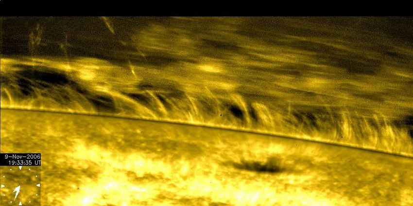
© G. Schneider and J. Moskowitz 2006
http://nicmosis.as.arizona.edu:8000/ECLIPSE_WEB/ECLIPSE_06/TSE2006_REPORT.html
The chromosphere: gateway to the corona ?
… Or the purgatory of solar physics ?
Judge (2010) clickable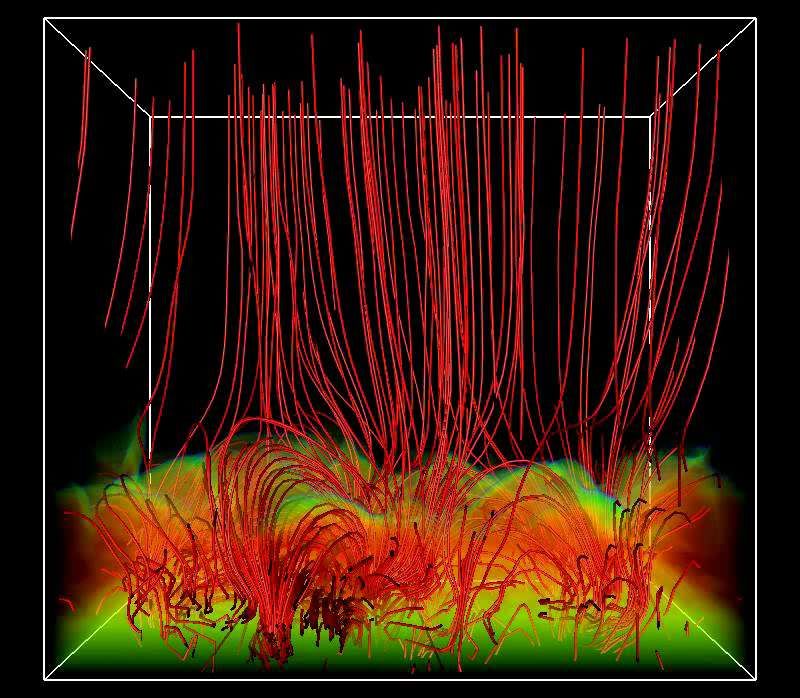
A fiery purgatory in medieval

Purgatory is purification
in which the souls are
made ready for Heaven.

                     The Very Rich Hours of the Duke of Berry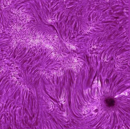
The chromosphere: gateway to the corona ?
“We do not understand from first principles why the Sun
is obliged to manifes these phenomena.”
“Variable (chromospheric) UV influences the heliosphere,
including the Earth’s atmosphere.”
… Or the purgatory of solar physics ?
Judge (2010) clickable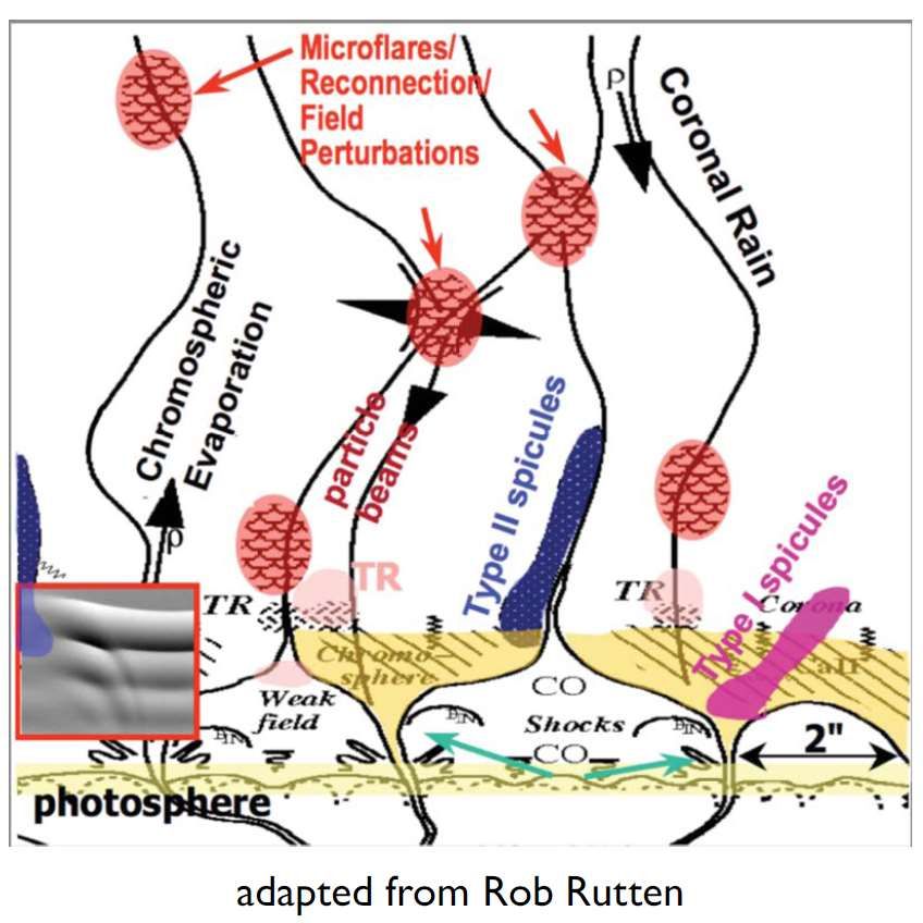
Flash slitless spectrum
              D1 D2

• reveals spectral lines formed in the chromosphere
• the chromosphere is optically thick (i.e., observable on the disk) in
  the lines seen in the flash spectrum

               spectrum: EurAstro Team, Rutten (2010)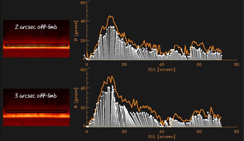
Flash slitless spectrum
              D1 D2

• reveals spectral lines formed in the chromosphere
• the chromosphere is optically thick (i.e., observable on the disk) in
  the lines seen in the flash spectrum

                There are two exceptions. Which ?

               spectrum: EurAstro Team, Rutten (2010)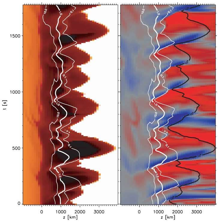
Flash slitless spectrum
              D1 D2

• reveals spectral lines formed in the chromosphere
• the chromosphere is optically thick (i.e., observable on the disk) in
  the lines seen in the flash spectrum

                There are two exceptions. Which ?

• Na I D1 & D2 NOT chromospheric due to scattering source function
                   (see Uitenbroek & Bruls, 1992)
• He I D3 NOT seen in the disk spectrum

               spectrum: EurAstro Team, Rutten (2010)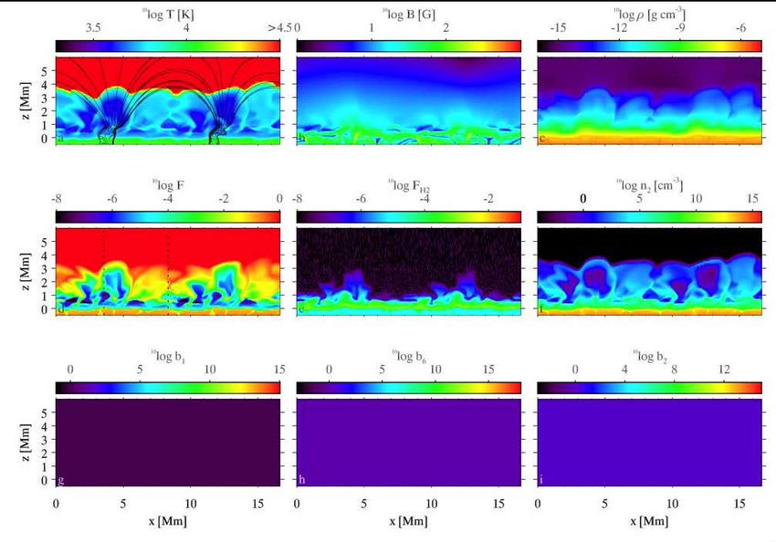
Principal chromosphere diagnostics
             D1 D2

• visible:     Hα, resonance lines Ca II H & K

• UV:          Mg II k & h 2796 & 2803 Å ( Mg II core-to-wing index )
               Ly α 1216 Å, He II 304 Å

• IR:          triplet Ca II 8498, 8542, 8662 Å
               triplet He I 10 830 Å

               spectrum: EurAstro Team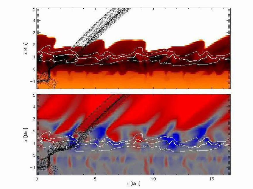
Chromosphere at high resolution
Spicules come at the stage
Hinode
Pgass nkT
2
Pmag B
8
lower chromosphere
bellow 1300 km: β > 1
Ca II H
Centeno et al. (2008) spicules: βSpicules at very high resolution
Hinode Ca II H
Lippincott (1957)
Bray & Loughhead (1974)What drives spicules ?
Lippincott (1957)
Bray & Loughhead (1974)
hmax 9 800 km vmax 24 km s-1
v max 2 v max 2g h max 73 km s-1
But : h max 1050 km
2g
g – solar gravity: 274 m s-2
Unknown driver propels spicules along their trajectories.Off-limb fine structures
spicules of type I and II
macrospicules
surges
Hinode Ca II H
DOT Ca II H
SoHO/SUMER O V Wilhelm (2000) Tziotziou et al. (2005)On-disk fine structures
Active regions:
• (dynamic, Hα) fibrils
• (bright, Ca II K) fibrils
• disk spicules
• grains
• (dynamic, Lyα, X-ray) jets
• (anemone, ) jets
Y
Quiet Sun:
• (dark, bright) mottles
Groups of mottles:
• rosettes
• bushes
• chains
The latest species:
• straws
line center of Hα • rapid blueshifted events
• black beadsOverview of the talk
1. Observations
a) from the ground
• imaging ( SST, DST, DOT )
• spectroscopy ( SST )
• spectropolarimetry ( VTT )
b) from space
• Hinode
c) simultaneous from the ground and space
• DST + SDOOverview of the talk
1. Observations
a) from the ground
• imaging ( SST, DST, DOT )
• spectroscopy ( SST )
• spectropolarimetry ( VTT )
b) from space
• Hinode
c) simultaneous from the ground and space
• DST + SDO
2. Theory and simulations
• brief hindsight on 1-D simulations
• the latest 2-D simulations
• non-equilibrium time-dependent ionization of hydrogen
• solar atmosphere cartoonsOverview of the talk
1. Observations
a) from the ground
• imaging ( SST, DST, DOT )
• spectroscopy ( SST )
• spectropolarimetry ( VTT )
b) from space
• Hinode
c) simultaneous from the ground and space
• DST + SDO
2. Theory and simulations
• brief hindsight on 1-D simulations
• the latest 2-D simulations
• non-equilibrium time-dependent ionization of hydrogen
• solar atmosphere cartoons
3. The new window into the chromosphere
• Atacama Large Millimeter/submillimeter Array ( ALMA )
• simulations of the solar chromosphere at millimeter and
submillimeter wavelengthsState-of-the-art imaging of the chromosphere
Swedish 1-m Solar Telescope
+ adaptive optics
+ image postprocessing
diagnostics: H line center
date: October 4, 2005
duration: 72 min
Resolutions
temporal: 3 frames per second
spatial: 70 – 100 km
Field of view:
61 arcsec 61 arcsec
Main result:
Hα image sequence with the
highest resolution ever
achieved.
van Noort & Rouppe van der Voort (2006)Dynamic fibrils in H
Hansteen et al. (2006) De Pontieu et al. (2007)
Main results:
• confirmed extensions and retractions
• confirmed parabolic top trajectories
• linear relationship between maximum velocity and deceleration
• Hα dynamic fibrils in a plage co-spatial with areas of increased power of 5-min
oscillations
• field-aligned magnetoacoustic shock excitationCa II 8542 Å - a new diagnostics
of chromospheric fine structures
Dunn Solar Telescope
+ IBIS (Interferometric BImodal Spectrometer)
1 October 2005
Main results:
• discovery of fibrils in Ca II IR lines
• close similarity of Hα and Ca II IR fibrils
Cauzzi et al. (2008)Multispectral tomographic observations Control room of the Dutch Open Telescope
Multispectral tomographic observations
                       Speckle image reconstruction

                              Speckle code

 Control room of the
                       Computer cluster for fast
Dutch Open Telescope
                        image reconstruction
Demo of speckle reconstruction
Hα – line center
http://dot.astro.uu.nl/DOT_speckle.htmlMultispectral tomographic observations
Speckle image reconstruction
Speckle code
Control room of the
Computer cluster for fast
Dutch Open Telescope
image reconstructionA sunspot in the DOT style
photosphere in the G band
date: 7 June 2006
duration: 1 hour
upper photosphere
+
lower chromosphere in Ca II H A sunspot in the DOT style
the solar chromosphere in Hα
above a sunspot
blue wing of Hα - 0.7 Å
upward motions
red wing of Hα + 0.7 Å
downward motions
Hα centerSpectroscopy of dynamic fibrils
in Hα and Ca II 8662 Å
Hα Ca II 8662 Å slitjaw DOT Hα image
Swedish 1-m Solar Telescope
Velocity-time plot +TRIPPEL spectrograph + Adaptive
for Ca II 8662 Å . Optics + Dutch Open Telescope
date: 4 May 2006
Dynamic fibrils duration: 40 min
seen as diagonal cadence: 0.5 s
dark components Main result: Extensions and
across the retractions of dynamic fibrils are actual
spectral line. mass motions.
Langangen et al. (2008)The magnetic field of off-limb spicules
Stokes I
Stokes Q
the slit of spectrograph
Stokes U
German VTT + TIP
He I 10 830 Å triplet
17 August 2008
Stokes V
Centeno et al. (2008)The magnetic field of off-limb spicules
telescope + instrument: German Vacuum Tower Telescope + TIP
date of obseravtion: August 17, 2008
diagnostics: He I 10 830 Å triplet
Main results:
• measurements of magnetic field strengths of spicules
• 48 G (left panels), 9 G (right panels)
Centeno et al. (2010)The magnetic field of off-limb spicules
the slit of spectrograph
Centeno et al. (2008)Spicules in the Hinode/SOT style telescope: Solar Optical Telescope ( 50 cm) diagnostics: Ca II H Main result: discovery of two fundamntally different types of spicules
De Pontieu et al. (2008)
Anemone jets in Ca II H by
                   Hinode/SOT

Anemone japonica

                      Shibata et al. (2007)
Anemone jets in Ca II H by
Hinode/SOT
Shibata et al. (2007)Inverted Y-shape jets
implying magnetic reconnection
Shibata et al. (2007)Giant anemone jet in multispectral
observations and simulations
Nishizuka et al. (2008)Multispectral tomography
of the solar atmosphere
photosphere
DST/IBIS line wing of Fe I 5434 Å 3 August 2010Multispectral tomography
of the solar atmosphere
upper
photosphere
+
transition
region
SDO/AIA C IV + continuum 1600 Å 3 August 2010Multispectral tomography
of the solar atmosphere
upper
photosphere
+
lower
chromosphere
DST/IBIS line wing of Ca II 8542 Å 3 August 2010Multispectral tomography
of the solar atmosphere
chromosphere
APOD
2 November 2010
DST/IBIS line center of Ca II 8542 Å 3 August 2010Multispectral tomography
of the solar atmosphere
chromosphere
DST/IBIS line center of Hα 6563 Å 3 August 2010Multispectral tomography
of the solar atmosphere
chromosphere
+
transition region
SDO/AIA He II 304 Å, T = 50 000 K 3 August 2010Multispectral tomography
of the solar atmosphere
transition region
+
corona
SDO/AIA Fe IX 171 Å, T = 650 000 K 3 August 2010wavelengths
Dataspace
to live in
timeOverview of the talk
1. Observations
a) from the ground
• imaging ( SST, DST, DOT )
• spectroscopy ( SST )
• spectropolarimetry ( VTT )
b) from space
• Hinode
c) simultaneous from the ground and space
• DST + SDO
2. Theory and simulations
• brief hindsight on 1-D simulations
• the latest 2-D simulations
• non-equilibrium time-dependent ionization of hydrogen
• solar atmosphere cartoons
3. The new window into the chromosphere
• Atacama Large Millimeter/submillimeter Array ( ALMA )
• simulations of the solar chromosphere at millimeter and
submillimeter wavelengthsEquations of 1-D hydrodynamics
of spicules
Sterling (2000)Numerical spicule models
• strong pulse in the lower atmosphere (the photosphere or low chromosphere)
• weak pulse in the lower atmosphere (rebound shock model)
• pressure-pulse in the middle or upper chromosphere
• Alfén wave models
Corona
TranReg
initial temperature at t = 0 A model spicule produced by a pressure
pulse in the low chromosphere
initial density at t = 0
Sterling (2000)Numerical hydrodynamics of
spicules
Temperature Density Velocity
Suematsu et al. 1982: SolPhys, 75, 99.Numerical hydrodynamics of
spicules
Temperature Density
Main results:
• the shock is strong
enough to uplift
theTransReg – Corona
interface
• the matter following
behind the interface is
identified as a spicule
• the model explains the
generation, height and
density of spicules
Suematsu et al. (1982)Alfvén wave model of spicules and
coronal heating
Kudoh & Shibata (1999)Alfvén wave model of spicules and
coronal heating
Density
B
BS
Kudoh & Shibata (1999)Alfvén wave model of spicules and
coronal heating
Density
Main results:
If the root mean square of the perturbation is
greater than 1 km s-1 in the photosphere:
• the transition region is lifted up to more
than 5000 km (i.e., the spicule is
produced),
• the energy flux enough for heating the
quiet corona (310-5 ergs s-1 cm-2) is
transported into the corona
Kudoh and Shibata 1999: ApJ, 514, 493.N-shaped magnetoacoustic shocks
1 2
Ekin v const .
2
Reduction of the effective gravity along tilted magnetic channels:
lowering of cutoff frequency
propagation of p-modes into the chromosphere as N-shaped shocks
repetitive lift of chromospheric-transition region interfaceDynamic fibrils in H
Hansteen et al. (2006) De Pontieu et al. (2007)
Main results:
• confirmed extensions and retractions
• confirmed parabolic top trajectories
• linear relationship between maximum velocity and deceleration
• Hα dynamic fibrils in a plage co-spatial with areas of increased power of 5-min
oscillations
• field-aligned magnetoacoustic shock excitationNumerical 1-D simulations of shock
wave-driven chromospheric jets
• 1-D magnetohydrodynamics (MHD) simulations
• choosen magnetic field strength: 60 G (610-3 T)
• choosen field inclinations: 0, 30, 45, 60
• choosen piston periods: 180 s, 240 s, 300 s, 360 s
• choosen initial amplitudes: 200 ms-1, 500 ms-1, 800 ms-1, 1100 ms-1
Heggland et al. (2007)Numerical simulations of shock
wave-driven chromospheric jets
TranReg
Chrom +
Corona
tops of jets
Main results reproduce:
• parabolic shapes of Chrom – TranReg interface
• the range of observed decelerations and roughly max. velocities
This gives strong support that fibrils are driven by magnetoacoustic shocks.
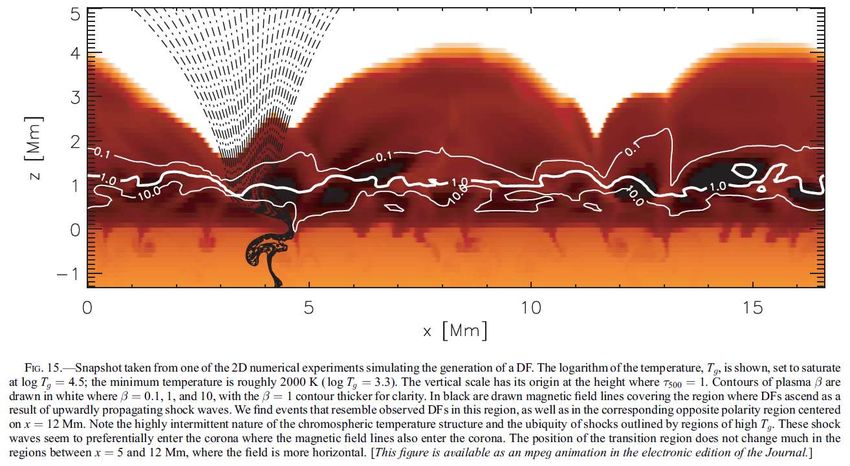
Heggland et al. (2007)Numerical 2-D MHD simulations
of dynamic fibrils
De Pontieu et al. (2007)Numerical 2-D MHD simulations
of dynamic fibrils
De Pontieu et al. (2007)Time-slice plot of Time-slice plot of
temperature vertical velocity
within dynamic within dynamic
fibril at x = 4 Mm fibril
blue – upflow
red – downflow
bi-directional
De Pontieu et al. (2007)Numerical 2-D MHD simulations
of dynamic fibrils
observation simulation
Main results:
• striking similarities of observed and simulated values for deceleration, maximum
velocity, maximum length, and duration of dynamic fibrils
• this strongly suggests that dynamic fibrils are formed by upwardly propagating
waves generated in the photosphere as a result of p-mode oscillations
De Pontieu et al. (2007)Non-equilibrium hydrogen ionization in MHD simulations of the solar atmosphere Radiative heating/cooling: + equation of chemical equilibrium + equations of charge, internal energy, and particle (hydrogen nucleus) conservation
Why non-equilibrium time-dependent
hydrogen ionization ?
Since characteristic dynamic times of
chromospheric fine structures are much shorter
than time necessary to establish statistics
equilibrium of hydrogen ionization.
In other words, the timescale on which the
hydrogen level populations adjust to changes in
the atmosphere is too long compared to the
timescale on which the atmosphere changes.
Swedish 1-m Solar Telescope
diagnostics: H line center
date: October 4, 2005
duration: 72 min
Resolutions - temporal : 3 frames per second
- spatial: 70 – 100 km
van Noort & Rouppe van der Voort (2006)Non-equilibrium hydrogen ionization in 2-D
simulations of the solar atmosphere
Leenaarts et al. (2007)Non-equilibrium hydrogen ionization in 2-D
simulations of the solar atmosphere
Main results:
• non-equilibrium H ionization is
essential in simulations because
the resulting temperature
structure and hydrogen
populations differ dramatically
from their LTE values
• the degree of ionization of H in
the chromosphere does not
follow the local T
• the next step is to compute Hα in
detail from this simulation (not
yet done)
Leenaarts et al. (2007)Numerical 3-D MHD simulation from
the photosphere up to the corona
De Pontieu et al.: 2007, Science, 318, 1574.Next frontier – to reproduce similar Hα images in numerical simulations
Solar atmosphere cartoons in time

            Ayres et al. (2009)
Solar atmosphere cartoons in time
De Pontieu et al. (2008)Overview of the talk
1. Observations
a) from the ground
• imaging ( SST, DST, DOT )
• spectroscopy ( SST )
• spectropolarimetry ( VTT )
b) from space
• Hinode
c) simultaneous from the ground and space
• DST + SDO
2. Theory and simulations
• brief hindsight on 1-D simulations
• the latest 2-D simulations
• non-equilibrium time-dependent ionization of hydrogen
• solar atmosphere cartoons
3. The new window into the chromosphere
• Atacama Large Millimeter/submillimeter Array ( ALMA )
• simulations of the solar chromosphere at millimeter and
submillimeter wavelengthsModel of the quiet solar atmosphere
corona transition chromosphere photosphere
region
VAL3C
Vernazza et al. (1981)Model of the quiet solar atmosphere
corona transition chromosphere photosphere
region
VAL3C
Vernazza et al. (1981)ALMA – the new window into the solar chromosphere • ALMA = Atacama Large Millimetre/submillimetre Array • operated by ESO • 66 antennas with diameters 12 m and 7 m • planned full operation in 2012
ALMA – the new window
into the solar chromosphere
• main ALMA target - cold universe
• also observations of the solar chromosphere and its fine structures
• expected FoV on the Sun: 21 arcsec at = 1 mm
• expected spatial resolution: 1.27 arcsec at = 3 mm
0.42 arcsec at = 1 mm
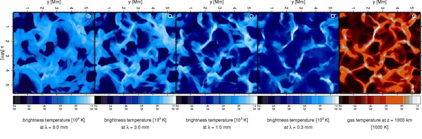
0.13 arcsec at = 0.3 mmSimulations of inter-network regions
of the Sun at millimetre wavelengths
Why is the chromosphere in millimeter wavelengths so atractive ?
Since the source function is Planckian, thus easy LTE (but not opacity).
“ALMA is promising tool for imaging the chromospheric fine-structure at high
cadence.”
“Application of ALMA is broad and includes the study of the fine-structure of
the magnetic network, too.”
Wedemeyer-Böhm et al. (2007)You can also read