Solar Physics from Kodaikanal Observatory - Jagdev singh, Indian Institute of Astrophysics, Bengaluru - FTP Directory Listing

Solar Physics from Kodaikanal Observatory

                     Jagdev singh,
      Indian Institute of Astrophysics, Bengaluru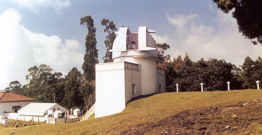

Beginning of the Solar Physics Observatory, Kodaikanal
• Kodaikanal Observatory traces its history back to 1787, when William Petrie, an
  officer of the Company, with two 3-in achromatic telescopes, two astronomical
  clocks with compound pendulum and a transit instrument started observing the
  stars at Madras (Chennai).
• It was started to promote the knowledge of astronomy, geography and
  particularly, navigation so that ships coming to India find their way easily.
• In 1879 a committee known as “Solar Physics Committee” was formed to suggest
  the ways to study the sun.
• Committee recommended to take the photographs of the sun frequently and to
  begin the spectrographic observations of the sun.
• One of the objective was to study the activity on the sun, particularly the sunspots
  and their relationship to the rainfall. Government had supported this program in
  the belief that a study of the Sun would help in the prediction of the monsoons,
  their success and failure, the failure often lead to famines (draught conditions).

White Light images of Sun
                • Telescope = 15cm aperture
                • Image Size = 200 mm
                • Data = Since 1904 to till today

                •Research Topics
                •Study of solar activity and its variation with time
                •White light Faculae and cycle prediction
                •Study of solar rotation and differential rotation
                •Variation of solar rotation with solar cycle phase
                •Rotation rate of young spots
                •Rotation rate of well developed spots
                •Correlation between sun spot area and other features e.
                g. Ca-K index, UV and EUV irradiance, 10-cm Index
                •Variation in tilt angle (Joy’s law)
                •Space weather predictions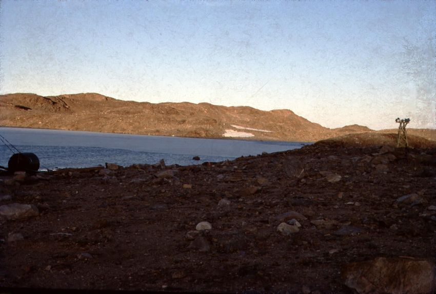

Spectro-heliograph & Shelton’s Clock
                    • Two parts, One Ca-K & other H-alpha
                    • Objective makes image on the slit
                    • Broad-band filter isolates different
                    wavelength
                    • Collimators makes the beam parallel
                    • The parallel beam then falls on a
                    disperser ( Prism or Grating)
                    • Second slit separates the wavelength-
                    band (pass-band) for making the image
                    • Curvature corrector corrects the curvature
                    in spectral line
                    • The photographic plate is kept just after
                    the second slit.
                    • The whole system moves across the image
                    with uniform speed controlled by hydraulic
                    system.
                    •The speed is controlled by an oarfish
                    whose opening can be adjusted.
                     Image is formed on the plate – step by step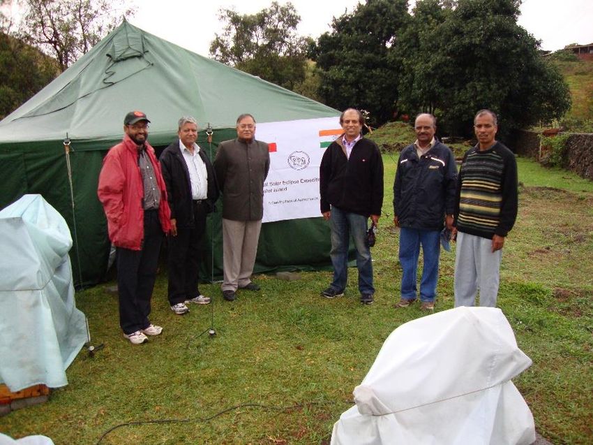

Spectro-heliograph & Science

                                                      H-alpha image

Study of Solar activity, Flares, Prominences, Filaments, Dynamics
of filaments with solar cycle phase, Heating of filaments before
disappearing, Magnetic Neutral Lines using the Large-scale Solar
Activity, Poleward migration of the magnetic neutral line and the
reversal of the polar fields on the sun, Do polar faculae on the
sun predict a sunspot cycle?, Space weather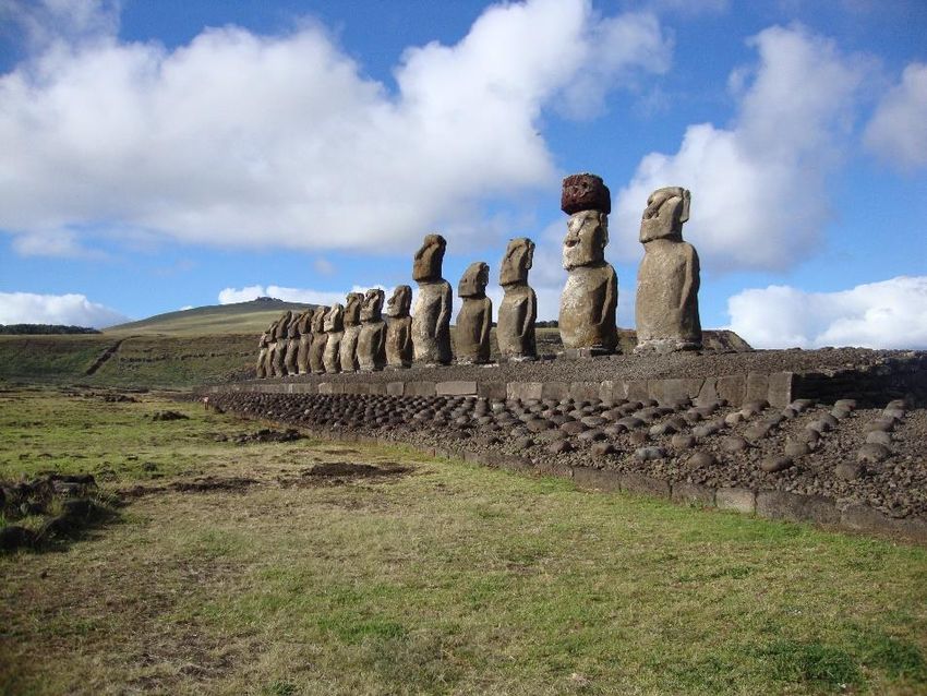

Discovery of Evershed effect

Discovery of radial flow in sunspot penumbra
 • John Evershed took the spectra of sunspots on January 5, 1909 and found
   that absorptions lines are tilted, specially in penumbra region of the sunspots
 • Subsequently he found the similar tilt of the absorption lines when he kept
   the slit at different angles in the sunspot region
 • Then he concluded it can be explained if the there is radial flow from central
   region to outer regions of the sunspot, known as “Evershed flow”. The flow
   velocity is about 2 Km / sec.
 • Later on reverse flow in the upper chromospheric layer of the sun has been
   found.
 • There are various models to explain the “Evershed flow”
 • Bhatnagar (1964, Ph.D. Thesis) made a detailed study of the Evershed effect
   using Zeeman insensitive lines of Ni I and Fe I and found maximum
   tangential velocity of 0.6 km/sec, in the sunspot penumbrae.
 • Detailed studies of prominences were made in addition to sunspot activity

Study using H-alpha images obtained at Kodaikanal since 1912
• In the year 1980, Makarov and Sivaraman started a program to determine the position of filaments
  using the H-alpha images obtained at Kodaikanal since 1912 and used this information as proxy to
  study the dynamics of magnetic field on the sun.
• They found the magnetic neutral line migrated towards the pole ward with a speed 4 – 29 m / sec
  and the speed appears to be related to the strength of solar cycle. (Solar Phys. 1983a, 1983b)
• Further they found that both the polar region had one polarity for the duration of 0.5 -1.5 years for
  different solar cycles.
• They found the direction of neutral line movement is same for low and high latitude zones on the
  sun (1989a, 1989b, 1989c).
• They also found that smaller is the period between the end of polar field reversal and the beginning
  of new cycle, the stronger will be the new cycle.
• They confirmed that the velocity of poleward migration is a linear function of the ‘strength of the
  solar cycle’ (Solar Phys. 2001).
• They found that the duration of polar activity is more in even solar cycles than in odd cycles
  whereas the maximum Wolf numbers Wmax is higher for odd solar cycles than for even cycles
  (Solar Phys. 2003)

Detailed Study of rotation and differential rotation using sunspots
• In the year 1990, Sivaraman, Howard and Gupta planned to determine the
  sunspot locations using the photoheliograms obtained at Kodaikanal since 1904
  using a digitizer.
• They studied in detail the rotation rate and differential rotation rate using this
  digitized data (Solar Phys., 1993, 1999a, 1999b)
• They found the tilt angles ( angle between leading and following sunspot groups
  with respect to the equator of the sun) differ between the north and south
  hemispheres ( Solar Phys. 1999c)
• Further, they found that tilt angle depends the size of the sunspot group (Solar
  Phys. 2000).
• They also found the variation in the rotation rate of sunspots with the age of the
  sunspot group (Solar Phys., 2003)
• Fast variations in the sunspot groups, such as rotation of the group has been
  found to be cause of triggering of flares and prominence eruptions (
  Sundararaman, Selvendran and others).

Discovery of Large convective cells (Super-granules)
                  • Leighton (1959) developed a new technique to study
                    the magnetic field on the sun and found the
                    agreement between magnetic field pattern and Ca-K
                    line emission pattern (plage areas).
                  • Simon and Leighton (1962) discovered the existence
                    of large convective cells, known as “super-granules”.
                    The mean size being ~30,000 Km with horizontal
                    flow velocity ~ 0.4 Km / sec., from the center
                    towards edges of the cell.
                  • These cells have the similarity in appearance with
                    the Ca-K network.
                  • These cells have an average life time of ~ 20 hours.
                  • Simon and Leighton (1964) found the existence of 5
                    min oscillations in the vertical component of the
                    velocity.

Study of Super-granules (Ca-K network) using Ca-K images
• With this back ground Singh and Bappu in the year 1977 started to look for the methodology
  to determine the average size of Ca-K network reliably. They experimented with different
  techniques such as, equal density contours, use of mm grid and enlarged images etc.

•Using the long series of data available at Kodaikanal, Singh & Bappu (1981)
found that Ca-K network cell size varies with the phase of solar cycle being small
during the maximum phase by about 5% as compared to that at minimum phase.

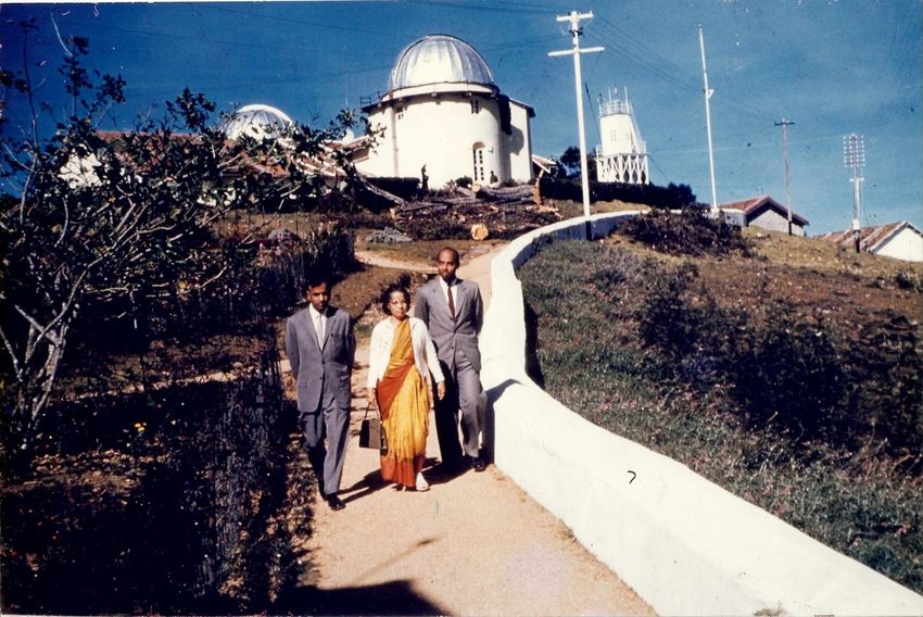
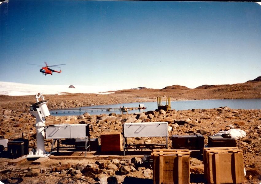
Why Antarctic Expedition
    • It has been found that average life-time of Ca-K
      network representing super-granules is about 20
      hours. Day & night cycle on most of the developed
      places on the earth does not permit to study the
      complete history of the super-granules.
    • Alternatively, one can go to space, Arctic or Antarctic
      region to make such a study. India has established a
      permanent center, known as “Maitri” in Antarctic
      region from where one can observe sun at mid-night.
    • We, therefore, planned an expedition to “Maitri” to
      obtain the images of the sun in Ca-K line
      continuously, 24 hours a day with out any gap.
    • It took our team consisting of 26 scientists from
      various research fields ~ 25 days to reach Antarctica
      by a dedicated ship from Goa.

Sky conditions at Mid-night

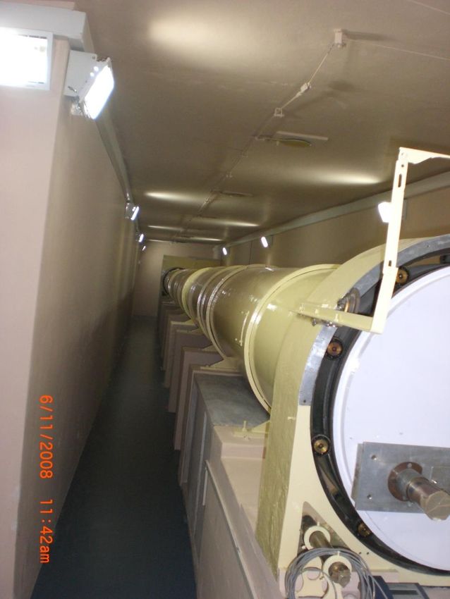
Details of the Instrument
                                       •15-cm plan mirror
                                       • 15-cm folding mirror
                                       •12.5-cm aperture with 300-cm
                                       focal length objective lens
                                       •1.2 A pass-band Day-star filter
                                       •Minolta camera-body fitted with
                                       timer to record the epoch of
                                       exposure automatically.
•Heliostat reflects light from sun     •Time sequence images with an
parallel to the rotation axis of the   interval of 5 minutes for longer
Earth.                                 stretch for days & also with 1
•Can track the sun 24-hours a day      minutes for shorter stretch of few
•Mirror rotates at 15-degrees/ hour    hours
•Image rotates at the image plan
•We need to help in down loading the
helicopter even during observations

Ca-K line images of the sun obtained from Antarctica

                                     •Data obtained for 106
                                     hours with a gap of about
                                     45 minutes everyday (24
                                     hours).
                                     •Data used to study the
                                     life of Ca-K networks.
                                     •To compare the lifetime
                                     in active and quiet
                                     regions on the sun.
                                     •The data has been used
                                     for other investigations
                                     also

Lifetime of the active and quiet cells

                    • To summarize the results of the
                      analysis of 106- hour continuous time
                      sequence of Ca-K filter-grams
                      obtained at the Indian permanent
                      station “Maitri” in the Antarctic
                      region shows that:
                    • The most probable lifetime of Ca-K
                      network cell is about 22 hours.

Relation between the cell size & its lifetime for quiet
                       region and Active region cells

• There exists a correlation between the lifetime and cell size such that bigger
  cells live longer
• Cells (of a given size) associated with active regions live longer than those in
  quiescent regions.

Other results - data from Antarctica and Kodaikanal
• Using Temporal auto-correlation function (ACF) of the time series of 106 hours
  obtained from Antarctica Raju, Srikanth and Singh (1998) found the lifetime of
  network cells depends on the activity of the region. The estimated lifetimes are 24–
  34 hours for quiet-region cells and 58–61 hours for active-region cells. They also
  showed the existence of long-period oscillations in the solar atmosphere.
• Srikanth, Raju and Singh (1998) using the Antarctica data and found a linear
  dependence of lifetime on cell area, with a least squares fit slope of 3.34 x 107 km2
  hr-1. This relation can be explained by assuming the network evolves by means of a
  diffusion process of the magnetic elements.
• Srikanth and Singh (2000) studied the distribution of super-granule sizes in detail
  and found the evidence for the existence of meso-granules with size of ~10000 Kms.
• From the Ca-K images obtained at Kodaikanal they found that the size of the cells varies with
  latitude being minimum at about 20o latitude.
• Paniveni et al . (2010) determined the fractal dimension D for supergranulation using the relation ,
  P ∝ AD/2 where A is the area and P the perimeter of the super-granular cells from KKL, Ca-K
  images. They find a fractal dimension of about 1.12 for active region cells and about 1.25 for quiet
  region cells, a difference that could be attributed to the inhibiting effect of the magnetic field.

Variation of solar rotation with time using Ca-K plage areas
                                 • We created a time series of plage areas for
                                   10-15 and 15-20 latitude belts in both the
                                   hemispheres for the period of 1951-81.
                                 • FFT of the data of 512 data gave the average
                                   rotation rate for the belt.
                                 • We found that the average rotation rate
                                   varied with time in all the chosen four
                                   latitude belts.
                                 • There is good correlation between the
                                   adjacent latitude belts but no north south
                                   symmetry.
                                 • Several quasi-periodicities between 2- 11
                                   years were found in the rotation rate in these
                                   belts.
                                 • 7- year periodicity was found to be present in
                                   these belts as well as in the variation of total
                                   plage area on the sun.

Sidero-stat & Coelostat

Single mirror with the help of drive
system follows the sun and directs the
light to the fixed objective of large
focal length and the spectrograph /
spectro-heliograph. In this set up the
image of the sun rotates. In coelostat
the does not rotate but you need two
mirrors of high quality.

Solar tower telescope (STT) at Kodaikanal

M1, M2 & M3 = 60 cm Flat mirrors; Objective aperture = 38
cm; Focal length = 36.6 m; F -ratio = 96

STT & Science
        High resolution spectroscopy
        Grating as the disperser with

       600 lines/mm blazed at 4th
       order green
        Littrow configuration

        Spectro-polarimetry

       Study of Evershed Flow

       Study of oscillations in

       intensity & velocity
       Sun as star in Ca-K line

       Ca-K line profiles of the sun as a

       function of latitude and
       integrated over the longitude

Bappu and Sivaraman (1971)

                             •Comparing the images
                             and spectra of Ca-K line
                             obtained at KKL Bappu
                             and Sivaraman (1971)
                             concluded that bright fine
                             mottling is responsible for
                             the relation found by
                             Wilson & Bappu (1957)
                             between Ca-K emission
                             line widths and absolute
                             magnitude of stars.

Study of weak magnetic field on the sun
• Bhattacharyya (1970) developed a Babcock type magnetometer
  using circular polarizer in front of electro-optic modulator and
  photomultiplier tubes at the Solar Tower Telescope, Kodaikanal.
• He used it to study the velocity oscillations and life of bursts at
  different heights (up to 2220 Kms) by observing in Ni I, Fe I, Ti I,
  Ba II, Na I, Mg I and H-beta. He made observations in the range
  of 2 - 4 hours in each line.
• He found the mean duration of bursts in the lower chromosphere is
  ~ 14 minutes less than that for the photospheric lines ~31 minutes.
• He found that period of velocity oscillations for H-beta line is ~
  200 sec. while that for the photospheric lines is ~ 300 sec.
• Bhattacharyya, Saxena and Singh (1975) used the magnetometer to
  investigate the relation between the photospheric magnetic field
  and Ca-k network.

Study of 5-minute oscillations
• Simon and Leighton (1964) found the existence of 5 min oscillations in the
  vertical component of the velocity.
• After the study of Evershed flow by Bhatnagar (1964), Sivaraman started to
  plan the study of 5-minutes oscillations in detail following the discovery these
  by Simon and Leighton.
• Sivaraman made observations in three spectral bands, namely around 634,
  658.7 and 428 nm with high temporal resolution for 30 – 40 minutes during the
  period 1969 -71 during the excellent seeing conditions to study the oscillations
  as a function height on the sun.
• Using many lines of FeI, NiI, SiII, Ca I, C I, CH and telluric lines Sivaraman
  (1973) found that the period of velocity oscillations decreases with increase in
  height from the photosphere, being 304 sec. to 295 sec.
• In core of one of the Fe I line he found intensity oscillations similar to that of
  velocity oscillations.

Study of sun as-a-star by monitoring the Ca-K line
• Following his discovery of Wilson- Bappu effect in 1957; a relation
  between the absolute magnitude of stars and the Ca-K line-width , Bappu
  stared a long-term program to monitor the Ca-K line profiles of the sun
  as-a-star at the Solar Tower Telescope, KKL in the year 1969. He was the
  first to start such a program. Later, Livingston started this program in 1976
  at KPNO and Keil in 1976 at the Sac Peak Observatory in USA.
• The disk-averaged Ca -K profiles obtained at the Kodaikanal solar tower
  telescope for the period 1969- 1984 were used to study the chromospheric
  variations in the Sun as a star. The 1A index shows an increase of 18% and
  28% during the 20th and 21st solar cycles, respectively. The corresponding
  enhancements in the central intensity in the K line are 24% and 40%,
  respectively. (Sivaraman, Singh et al., 1987)

Normalization of profiles

All the profiles were normalized at the wavelength
centered around 3935.16 Å considering the residual
intensity of 13 % (White & Suemoto, 1968)

Results

Ca-K line profiles of sun as a function of latitude and
              integrated over visible longitudes
• Singh while analyzing the Ca-K line data of sun as a star and his study of
  variation of rotation rate at different latitudes, thought that it will be better
  to have information about the Ca-K profiles as a function of latitude on
  long-term basis.
• He developed a methodology to obtain the Ca-K line profiles as a function
  of latitude and integrated as a function of latitudes at the STT and started
  to monitor the Ca-K profiles on daily basis whenever sky conditions
  permitted the observations as a function of latitudes and integrated over the
  visible longitudes since 1986.
• The spectra were recorded on the photographic films till 1997 and later
  these were taken using CCD cameras.
• This way data were collected till 2011 on regular basis with some gaps
  when the telescope was used for other type of observations.

Variation of K1 width with time at different latitude (N)
 The plots of K1 width with
 time at latitudes with an
 interval of 10 degrees
 indicate maximum solar
 activity at different
 latitudes occur at different
 times. The maximum
 variation occurs around 15
 degree latitude and
 minimum variation occurs
 around 55 degree latitude.
 The variations with solar
 cycle in polar regions are at
 moderate level.

Variation of K1 width with time at different
      latitude in southern hemisphere

Variation of K2 width with time at different
                latitude in northern hemisphere
The trend of variations
 in K2 widths at all the
Latitudes with time is
similar to that in K1
Widths. But K1 is
Inversely related to K2
width. During the
active phase K1 width
increases whereas K2
width decreases as
compared to minimum
phase.

Variation of K2 width with time at different
      latitude in southern hemisphere

Distribution of K1 width for various
             latitudes for both the hemispheres
•FWHM of distribution is
30% for equatorial region
•FWHM of distribution only
6% for 55 & 65 degree
latitude belts.
•FWHM of distribution
11% for polar regions
• The magnitude of
variations is maxim around
20 degree latitude minimum
around 60 degree. It is not
clear why the Ca-K line
widths show such a
behavior with latitude.

Distribution of K2 width for various latitudes
          for both the hemispheres

Cross correlation function of K1 for latitude belts

The cross correlation coefficients of K1 width of various latitudes with K1 width
at 35° latitude belt as a function of phase difference indicate that Toroidal field
shifted with velocity 5.1 m s-1 (North) 7.5 m s -1 (South). The phase difference
between the maximum activity at polar regions and equatorial belts is ~5.5 years.

Table lists the maximum value of cross-correlation coefficients between two
belts, significance level in % and the phase difference in months.
     Latitude Belts      Correlation coefficient    Phase difference (months)
     80n & 35n          0.48 (99.9), 0.31 (98.7)    -92.1 1.7 ; 77.2 1.4
     65n & 35n          0.16 (82.4), 0.05 (32.34)   -47.4 4.0 ; 50.1 14.9
     55n & 35n          0.43 (>99.9)                -7.8 1.2
     45n & 35n          0.71 (>99.9)                 2.1 0.8
     35n & 35n          1                            0
     25n & 35n          0.85 (>99.9)                 7.8 0.6
     15n & 35n          0.84 (>99.9)                17.7 0.3
     05n & 35n          0.83 (>99.9)                28.8 0.7
     05s & 35s          0.81 (>99.9)                18.9 0.5
     15s & 35s          0.84 (>99.9)                  9.0 0.5
     25s & 35s          0.85 (>99.9)                  3.0 0.6
     35s & 35s          1                              0
     45s & 35s          0.23 (96.7)                  -6.9 1.5
     55s & 35s          0.50 (>99.9)                 12.0 2.4
     65s & 35s          0.09 (49.8), 0.40(99.7)     -88.2 1.1 ; 42.6 1.5
     80s & 35s          0.12(61.7), 0.22(93.7)      -99.0 8.7 ; 49.5 11.6

Cross correlation function of K1 widths for
          adjacent latitude belts

Correlation coefficients with adjacent latitude belts
 Latitude belts   Correlation coefficients   Phase difference (months)
80n & 65n         0.11 (70) ; 0.1 (70)       -57.9 0.04 ; 51.9 0.04
65n & 55n         0.1 (70)                    6.3 0.04
55n & 45n         0.41 (>99.9)               11.7 0.03
45n & 35n         0.70 (>99.9)               1.6 0.02
35n & 25n         0.84 (>99.9)               8.0 0.01
25n & 15n         0.89 (>99.9)               9.1 0.01
15n & 05n         0.89 (>99.9)               9.6 0.01
15s & 05s         0.89 (>99.9)               9.1 0.01
25s & 15s         0.91 (>99.9)               5.8 0.01
35s & 25s         0.85 (>99.9)               3.2 0.01
45s & 35s         0.22 (96)                  6.9 0.02
55s & 45s         0.17 (87)                  1.1 0.02
65s & 55s         0.33 (99.9)                4.3 0.03
80s & 65s         0.11 (70), 0.1 (70)        -0.5 0.04 ; -78.5 0.04

Summary of results
The new method of observing as a function of latitude and integrated
over 180° longitude developed at KKL observatory (Singh, 1989) has
been very effective to study the chromospheric long term variability
for the period of 1986 -2011 and its implication to meridional flows.
•Comparison of Ca-K line parameters of Sun as a star derived from
observations as function of latitude at KKL with those obtained at
Kitt peak and NSO/Sac peak observatories shows a good agreement.
•Average value of K1 width during the maximum phase of the solar
cycle 22 is 0.673Å and 0.672Å for cycle 23.
•The mean value of K1 width is larger during minimum phase of
cycle 22 (0.55 ± 0.01Å) as compared to mean value of K1 width
(0.53 ± 0.01Å) for cycle 23 implying that decrease in solar flux,
probably due to very long term decrease in activity or extended
minimum after cycle 23 .

Continue.
•The values of K1 width for the activity phase are larger by about
10-15% than those for the quiet phase for the equatorial region up
to ~ 35° latitude.
•In the polar regions K1 width is 1-2 % smaller during the active
phase of the sun than that at minimum phase indicating more
activity at polar region during the minimum period .
•No symmetry in the northern and southern hemispheres in terms
of the speed of shifting of activity towards equator.
•The speed of shift of activity due to poloidal field towards polar
regions varies with time and complex.
•Less variation in the poloidal field ~ 60° latitude belt as compared
to those for the polar regions with the solar cycle is unexpected
and reason for this need to be explored.

Solar Activity and Meridional flow
The observed systematic variation in the activity on the solar surface has been
used to study recycling of two components of magnetic fields namely, the
toroidal and poloidal components through meridional flow (Choudhuri et al.
1995). The flow of material in the meridional plane from the solar equator
towards the Sun’s poles and from the poles towards the equator deep inside the
Sun to carry the dynamo wave towards the equator, plays an important role in
the Sun’s magnetic dynamo (Choudhuri et al. 1995; Charbonneau 2007).

                                     Artist's concept of the Sun's
                                     meridional circulation, a large
                                     scale flow that transports solar
                                     plasma from the equator to the
                                     poles and back like a giant
                                     conveyor belt.
                                     Credit: Science@NASA.

Conclusion
 In view of transport of magnetic flux (the solar activity)
from one latitude to other latitudes by the meridional
flows (Choudhuri et al. 1995), we propose the following
scenario. From these results we can conclude the
existence of multiple cell model for meridional flows. We
infer three types of cells. One those transports torodial
flux from mid latitudes to equatorial belts, second those
transport polodial flux from mid latitude to high latitude
belts up to ~ 60° and the third those exist in the polar
regions. Sindhuja, G. ; Singh, Jagdev; Ravindra, B.,
2014, ApJ, 792, 22.

Digitization unit developed at Kodaikanal
                • 1 m Labsphere with exit port 35 cm
                • Uniformity of light 1% from center to edge of the
                exit port
                • Current control to stabilize the intensity of source
                • Imaging Lens : Negligible vignetting
                • CCD camera: Format 4K  4K
                •Pixel size 15 micron
                •Read out 16 bit
                •Image scale is 0.86 arcsec per pixel
                •Room conditions: Temperature, Humidity and dust
                controlled
                • While designing the digitizers, the requirement to
                study of networks was taken into account.

Ca-K line spectroheliograms and Analysis

Frequency distribution of intensity of Ca-K Images

                          • High contrast Images in the
                          top row show vignetting due to
                          instrument.
                          • High contrast images in the
                          middle row show the removal
                          of instrument vignetting.
                          • Plots show the intensity
                          distribution after correction due
                          limb darkening and after the
                          correction due to instrument.

Detection of Plages and Networks

                         First time done for a
                         long series of Ca-K
                         Data. Worden (1998)
                         did it for limited Sac
                         Peak data

Variation of intensity of plages and networks with time

  The power spectral analysis of the temporal variations indicate that intensity of
  plages varies with solar cycle phase and with very large period . It also shows
  that intensity of active network varies with about 11 year period (solar cycle).

TWIN TELESCOPE AT KODAIKANAL

H-alpha Telescope at Kodaikanal

Coronal Temperature
 • Million Degree – Observed from
   the continuum scattered light by
   electrons (scale height) as well as
   the emission lines from highly
   ionized species.
 • Edlen 1939 – Coronal Green
   Line.
 • Why so high temperature is yet to
   be solved?
• How to estimate the temperature?
• By determining the scale height and modelling.
• From the intensity ratio of emission lines of different
  spices such as 7892 [Fe xi] & 6374 [Fe x]. (or computing
  the abundances of different ions of same element.
• From the width of emission lines

Why Observe during the Total Solar Eclipses:
 •A rare event of the nature which lasts impression through out life
 •Natural laboratory to study the high temperature plasma
 •The observations with the minimum of background scattered light

This figure illustrates the
importance of the scattered
light for coronal
observations. Observing
sites with pure blue sky
(which is very rare to find)
gives a scattered light of
about 10-6. In contrast, the
solar eclipse provides a very
low level of scattered light.

Expeditions by Indian Institute of Astrophysics
• Feb 16, 1980 TSE, Locations:Jawalgera and Hosur in
  Karnataka ; Experiments
• Spectroscopy of the solar limb as a function of height
  to study the temperature gradient in the solar surface
  using 60 feet tower telescope
• High spatial resolution Photometry of solar corona
  using 21 focus lens
• Polarization measurements of solar corona using 3
  Polaroid's simultaneously
• Multislit spectroscopy of the solar corona to determine
  the temperature and dynamics in the red line
• Interferometry of solar corona in the green emission
  lines to determine temperature structure
• Spectroscopy of the chromosphere to study the
  dynamics of spicules
• Limb darkening measurements using photometer

July 22, 2009, Total Solar Eclipse, Anji, Shanghai, China
Experiments:
To study the existence of waves in the solar corona and their nature:
• Spectroscopy of the Solar Corona in the green and red lines, simultaneously
• Photometry of the Solar Corona in the green and red emission lines

July 22, 2009 Eclipse

July 11, 2010 Total Solar Eclipse at Easter Island, Chile

Development of Experiments over Time
•   1980   Image-intensifier Red line      Multislit Spectroscopy       Spatial
•   1983   Image-intensifier Red line      Multislit Spectroscopy       Spatial
•   1994   Image intensifier Red & green Multislit Spectroscopy         Spatial
•   1995          PMT         Continuum        1 location              10 Hz
•   1998          PMT         Continuum        4 location              50 Hz
•   2006          CCD Green & Red              Imaging                 0.3 Hz
                                             Only one limb
• 2009            CCD Green & Red              Imaging                 1.1 Hz
•                                All around the sun up to 1.5 solar radii
• 2009            CCD Green & Red              Spectroscopy             0.2 Hz
• 2010            CCD Green & Red              Spectroscopy            0.23 &
                                                                       0.9 Hz

• 2010     CCD Spectroscopy in H-alpha line as function of height      ~7 Hz
                      ( New Experiment)

A coronal region observed in [Fe x], [Fe xi], [Fe xiii]
      and [Fe xiv] lines but not simultaneously

Variation of Line width of
the four emission lines with
height above the limb in the
polar regions. The
magnitude of variation is
larger in polar regions as
compared to the equatorial
region except for the green
line

Variation of line widths of
red and green coronal
emission lines with height
above the limb up to 500
arcsec in the equatorial
region. The line widths do
not show any increase or
decrease with height after
about 250 arcsec

Typical variation of intensity
ratios of emission lines with
height for individual coronal
loops as Seen in the previous
slide by + mark

Expected Intensity Ratios
• The abundances of different Fe ions
  as function of temperature indicate
  that
• Intensity ratio of [Fe xi] to [Fe x]
  emission line should increase if the
  thermal temperature increases
• Intensity ratio of [Fe xiii] to [Fe x]
  emission line should increase steeply
  if the thermal temperature increases
• Intensity ratio of [Fe xiv] to [Fe x]
  emission line should increase more
  steeply if the thermal temperature
  increases

Empirical Model to
explain the above
discussed results of
systematic
observations during
the period 1997-2007

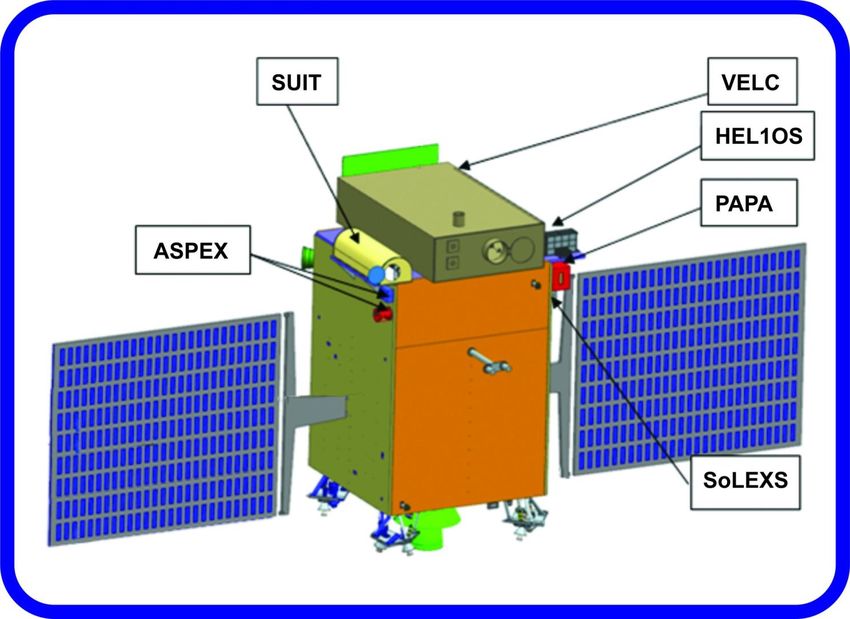
Aditya-1
1. Visible Emission Line
Coronagraph (VELC)
2. Solar Ultraviolet Imaging

Telescope (SUIT)
3. Solar Low Energy X-ray

Spectrometer (SoLEXS)
4. High Energy L1 Orbiting

X-ray Spectrometer (HELIOS)
5. Aditya Solar wind Particle

EXperiment (ASPEX)
6. Plasma Analyser Package

for Aditya (PAPA)
7 Mangnetometer

Scientific Objectives of space coronagraph

• Coronal waves and heating of the corona?
• Dynamics of Coronal loops: formation and evolution
• Temperature diagnostics of the corona (using line ratio
  techniques)
• Development and origin of CME’S
• Space weather Prediction
• Topology of magnetic fields
• Exploring the outer emission corona spectroscopically.

Aditya/VELC
VELC has an entrance aperture (EA) of 147 mm
primary mirror with clear aperture of 192 mm at

a distance of 1570 mm from the EA
M1 is an off axis parabola which focuses the

solar disc and corona onto M2
M2 is a concave mirror with a central hole

which allows the solar disc and coronal
radiations up to 1.05 solar radii to pass through
it.
Disc light is reflected by a M3 out of the

instrument through a small hole in a direction
perpendicular to EA (instrument top)
Coronal light reflected by M2 is collected and

collimated using a doublet lens.
The Lyot stop close to the collimator blocks the

radiations due to the diffraction at the EA.

Key Technologies

• Primary Mirror (

Thank you very much
   For your kind Attention

Discovery of Telescope
•Lippershey invented the telescope and
called his invention a "kijker", meaning
"looker" in Dutch and in 1608 applied for
the patent.
• Galileo made the telescope in 1609 and
discovered the sunspots on the sun. From
the movement of sunspots he concluded
that sun is rotating.

                        Spatial resolution
                         diffraction limit = 1.22 λ/D

                        ( In radian- convert into arcsec)

                         (1 arcsec = 720 km on sun)

                         Plate scale p = 1/f (arcsecs/mm)

                         Radian (in arcsec) / f in mm

                         Focal ratio F# = f/D

Simple telescope for observing Sun

                      •      Earlier Times
                      •Objective for imaging
                      •Shutter at the focal plan
                      •Broad band filter Red, Green, Blue
                      •Finder telescope
                      •Projection on a screen to centre
                      the image
                      •Magnifying lens
                      •Photographic Plate/Film to record
                      the image of sun
                      •   Present Times
                      •Computer controlled to point
                      •CCD cameras to record the image

Gravity Clock

                The telescope is driven
                by a gravity clock to
                track the sun or stars.
                A governor is used to
                control the speed of
                the telescope to
                compensate the
                seasonal variations in
                the velocity of earth
                around the sun.

Compact Telescopes

Generally used for observing the faint objects during the night time. But
now a days by taking care of heating near the secondary and focal plane,
these can be used to study the sun. The 40-cm telescopes were used to
observe the solar corona during the 2009 eclipse in China by taking images
of the corona in Red (6374 A) and Green (5303 A) lines. Spectroscopic
observations were also made in the red and green emission lines.

Solar Physics from Kodaikanal Observatory

              Jagdev singh

Imaging & spectroscopy