Southern Ocean cloud and aerosol data: a compilation of measurements from the 2018 Southern Ocean Ross Sea Marine Ecosystems and Environment ...
←
→
Page content transcription
If your browser does not render page correctly, please read the page content below
Earth Syst. Sci. Data, 13, 3115–3153, 2021
https://doi.org/10.5194/essd-13-3115-2021
© Author(s) 2021. This work is distributed under
the Creative Commons Attribution 4.0 License.

      Southern Ocean cloud and aerosol data: a compilation of
      measurements from the 2018 Southern Ocean Ross Sea
           Marine Ecosystems and Environment voyage
            Stefanie Kremser1 , Mike Harvey2 , Peter Kuma3,11 , Sean Hartery3 , Alexia Saint-Macary2,10 ,
           John McGregor2 , Alex Schuddeboom3 , Marc von Hobe5 , Sinikka T. Lennartz6 , Alex Geddes4 ,
        Richard Querel4 , Adrian McDonald3 , Maija Peltola7 , Karine Sellegri7 , Israel Silber9 , Cliff S. Law2,10 ,
          Connor J. Flynn8 , Andrew Marriner2 , Thomas C. J. Hill12 , Paul J. DeMott12 , Carson C. Hume12 ,
                              Graeme Plank3 , Geoffrey Graham3 , and Simon Parsons3
                                              1 Bodeker Scientific, Alexandra, New Zealand
                2 National    Institute of Water and Atmospheric Research (NIWA), Wellington, New Zealand
                                         3 University of Canterbury, Christchurch, New Zealand
                     4 National Institute of Water and Atmospheric Research (NIWA), Lauder, New Zealand
          5 Institute for Energy and Climate Research (IEK-7), Forschungszentrum Jülich GmbH, Jülich, Germany
                                  6 Institute for Chemistry and Biology of the Marine Environment,

                                             University of Oldenburg, Oldenburg, Germany
                            7 Université Clermont Auvergne, CNRS, LaMP, Clermont-Ferrand, France
                               8 School of Meteorology, University of Oklahoma, Norman, OK, USA
        9 Department of Meteorology and Atmospheric Science, Pennsylvania State University, University Park, PA,

                                                                   USA
                         10 Department of Marine Science, University of Otago, Dunedin, New Zealand
                                    11 Peter Kuma Software & Science, Christchurch, New Zealand
                   12 Department of Atmospheric Science, Colorado State University, Fort Collins, CO, USA

                          Correspondence: Stefanie Kremser (stefanie@bodekerscientific.com)

                                Received: 30 October 2020 – Discussion started: 9 November 2020
                             Revised: 13 May 2021 – Accepted: 31 May 2021 – Published: 2 July 2021

      Abstract. Due to its remote location and extreme weather conditions, atmospheric in situ measurements are
      rare in the Southern Ocean. As a result, aerosol–cloud interactions in this region are poorly understood and re-
      main a major source of uncertainty in climate models. This, in turn, contributes substantially to persistent biases
      in climate model simulations such as the well-known positive shortwave radiation bias at the surface, as well
      as biases in numerical weather prediction models and reanalyses. It has been shown in previous studies that in
      situ and ground-based remote sensing measurements across the Southern Ocean are critical for complement-
      ing satellite data sets due to the importance of boundary layer and low-level cloud processes. These processes
      are poorly sampled by satellite-based measurements and are often obscured by multiple overlying cloud layers.
      Satellite measurements also do not constrain the aerosol–cloud processes very well with imprecise estimation of
      cloud condensation nuclei. In this work, we present a comprehensive set of ship-based aerosol and meteorologi-
      cal observations collected on the 6-week Southern Ocean Ross Sea Marine Ecosystem and Environment voyage
      (TAN1802) voyage of RV Tangaroa across the Southern Ocean, from Wellington, New Zealand, to the Ross Sea,
      Antarctica. The voyage was carried out from 8 February to 21 March 2018. Many distinct, but contemporaneous,
      data sets were collected throughout the voyage. The compiled data sets include measurements from a range of
      instruments, such as (i) meteorological conditions at the sea surface and profile measurements; (ii) the size and
      concentration of particles; (iii) trace gases dissolved in the ocean surface such as dimethyl sulfide and carbonyl
      sulfide; (iv) and remotely sensed observations of low clouds. Here, we describe the voyage, the instruments, and

Published by Copernicus Publications.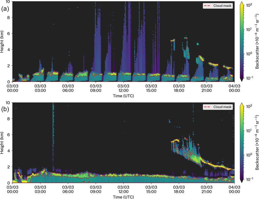
3116                                                              S. Kremser et al.: Measurements over the Southern Ocean

       data processing, and provide a brief overview of some of the data products available. We encourage the scientific
       community to use these measurements for further analysis and model evaluation studies, in particular, for stud-
       ies of Southern Ocean clouds, aerosol, and their interaction. The data sets presented in this study are publicly
       available at https://doi.org/10.5281/zenodo.4060237 (Kremser et al., 2020).

1   Introduction                                                   tor in this uncertainty (Myhre et al., 2013; Haynes et al.,
                                                                   2011). For example, Hyder et al. (2018) recently identified
The Southern Ocean is the cloudiest region on Earth and            that 70 % of the sea surface temperature biases observed
is also distant from major anthropogenic sources of aerosol        in model simulations, performed in support of the Coupled
(Haynes et al., 2011). This makes the Southern Ocean an            Model Intercomparison Project 5 (CMIP5), can be attributed
ideal environment for studying aerosol–cloud interactions          to the models not representing clouds and their properties
(Krüger and Graßl, 2011; Fossum et al., 2018; Hamilton             correctly. These errors occur because climate models simu-
et al., 2014) and the role of marine aerosol in the radiation      late too little cloud cover and contain biases in cloud albedo
budget. The contribution of marine aerosol to Earth’s radia-       over the Southern Ocean (Bodas-Salcedo et al., 2012; Schud-
tion budget is both direct, through aerosol scattering and ab-     deboom et al., 2019), resulting in projections that underes-
sorption, and indirect, via cloud droplet activation and their     timate the reflected solar radiation at the top of the atmo-
subsequent influences on cloud radiative processes (Murphy         sphere (TOA; Haynes et al., 2011) and overestimate down-
et al., 1998; Mulcahy et al., 2008; McCoy et al., 2015; Fos-       welling solar radiation at the ocean surface. This leads to
sum et al., 2018). Marine aerosol can be classified as pri-        excessive sunlight being absorbed by the ocean (Trenberth
mary or secondary in origin (Fossum et al., 2018). Primary         and Fasullo, 2010; Kay et al., 2016; Hyder et al., 2018) and
aerosols, such as sea spray, are directly injected into the at-    subsequent higher sea surface temperatures than observed
mosphere when breaking waves entrain air bubbles into the          (Bodas-Salcedo et al., 2012; Mechoso et al., 2016). Previous
ocean surface, which subsequently form whitecaps and burst         studies have also shown the importance of accurate mixed-
(Hultin et al., 2010; Salter et al., 2014). Secondary aerosols,    phase cloud parameterisations over the Southern Ocean in
such as sulfate aerosols, are formed from the nucleation of        climate models to properly simulate cloud radiative proper-
sulfur-containing gases in a gas-to-particle conversion pro-       ties over the Southern Ocean (Lawson and Gettelman, 2014;
cess. One of the main precursors of sulfate aerosol in the         Kay et al., 2016; Schuddeboom et al., 2019; Noh et al., 2019).
marine environment is dimethyl sulfide (DMS), a byprod-            In mixed-phase clouds, both liquid droplets and ice crys-
uct of an enzymatic compound produced within phytoplank-           tals coexist with the liquid water often being supercooled.
ton (dimethylsulfoniopropionate, DMSP; Read et al., 2008;          While observations in the Southern Ocean are sparse, mea-
Fossum et al., 2018). DMS is the main natural source of at-        surements reported by McCluskey et al. (2018); DeMott et al.
mospheric sulfur, with a global average of 28.1 Tg of sul-         (2018) and Welti et al. (2020) indicate that INP concentra-
fur being emitted annually from the oceans into the atmo-          tions are exceptionally low over the Southern Ocean, much
sphere in the form of DMS (Lana et al., 2011). When DMS            lower than previously estimated by Bigg (1973). The low
is emitted into the atmosphere, it undergoes a series of chem-     concentrations of INPs over the Southern Ocean limit cloud
ical reactions to form sulfur dioxide (SO2 ), resulting in a       droplet freezing, reduce precipitation, and enhance cloud
typical lifetime of DMS in the atmosphere of 1–2 d (e.g.           reflectivity compared to regions of higher INP abundance
Chen et al., 2018). The SO2 can then be further oxidised to        (e.g. Vergara-Temprado et al., 2018; Vignon et al., 2020).
form sulfuric acid, sulfate aerosol, and methanesulfonic acid      This indicates that an accurate representation of INPs in cli-
(MSA; e.g. Yan et al., 2020). Aerosol emitted into the atmo-       mate models is necessary to properly simulate cloud radiative
sphere can grow in size via condensation and coagulation.          properties over the Southern Ocean. For example, climate
The ability of any aerosol particle to serve as a nucleus for      models often produce too many ice crystals in mixed-phase
water droplet formation depends on its size, chemical com-         clouds that consume the liquid droplets and thereby change
position, the local supersaturation, and meteorological con-       the radiative properties of clouds (Kay et al., 2016). Further-
ditions such as the cloud base updraft velocity (Rosenfeld         more, due to the low INP concentrations identified to exist
et al., 2014). Aerosol has a significantly different impact on     broadly over the Southern Ocean, there is a need to better un-
cloud formation and evolution, depending on whether it acts        derstand secondary ice formation processes and their depen-
as ice-nucleating particles (INPs), cloud condensation nuclei      dence on INP concentration and to improve their representa-
(CCN), or both.                                                    tion in climate models. Observations support the embedded
   Despite their significant influence on climate, clouds still    occurrence of a variety of secondary ice formation processes
represent the largest source of uncertainty in modern climate      in clouds over the Southern Ocean, which are otherwise dom-
models with aerosol–cloud interactions being a major fac-          inated by supercooled water. These processes range from as-

Earth Syst. Sci. Data, 13, 3115–3153, 2021                                         https://doi.org/10.5194/essd-13-3115-2021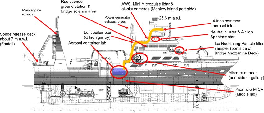
S. Kremser et al.: Measurements over the Southern Ocean                                                                        3117

sociation with seeding of ice crystals from colder cloud levels
that appears consistent with a rime splintering process (Fin-
lon et al., 2020) to studies suggesting the vital importance
of ice production via breakup following ice–ice collisions
(Sotiropoulou et al., 2021; Young et al., 2019).
   Reducing the uncertainty in the simulation of aerosol–
cloud interactions requires detailed observational data sets
against which models can be evaluated. However, this pro-
cess is hindered over the Southern Ocean by the lack of
ground-based and in situ measurements. While satellite-
based measurements can provide some data over the re-
gion, they cannot provide detailed aerosol chemical com-
position data or be solely relied upon to examine low-level
clouds (Kuma et al., 2021a; McErlich et al., 2020). There
have been only a limited number of ship- and ground-based
field campaigns over the Southern Ocean (see Table 1 for an
overview). Observational campaigns which provide detailed
measurements of low-level clouds, aerosol, aerosol precur-
sors, INPs, and CCN are essential for model evaluation, espe-
cially for parameters that can be indirectly estimated but not
accurately determined from satellite-based measurements.
   In this paper, we present a new data set of atmo-              Figure 1. The ship track of the RV Tangaroa with dates indicated
                                                                  by colours. The 2018 Southern Ocean Ross Sea Marine Ecosystem
spheric (cloud, aerosol, and thermodynamic properties)
                                                                  and Environment voyage extended from the North Island of New
and seawater measurements that were collected during              Zealand to off the coast of Cape Adare (Antarctica).
the 6-week Southern Ocean Ross Sea Marine Ecosys-
tem and Environment voyage (TAN1802) from Welling-
ton, New Zealand, to the Ross Sea, Antarctica, in 2018.           2     TAN1802 voyage – New Zealand to the Ross Sea
The data sets presented here are publicly available at
https://doi.org/10.5281/zenodo.4060237 (Kremser et al.,           The 2018 Southern Ocean Ross Sea Marine Ecosystem and
2020). Given the sparsity of data in the Southern Ocean re-       Environment voyage, TAN1802, was a voyage with NIWA’s
gion, this data set provides a valuable collection of atmo-       (National Institute of Water and Atmospheric Research) re-
spheric and underway measurements that can be used to             search vessel Tangaroa from Wellington to the Ross Sea be-
better understand aerosol–cloud processes over the South-         tween 8 February and 21 March 2018. The purpose-built re-
ern Ocean. This paper includes a description of DMS and           search vessel is 70 m long, with a beam width of 13.8 m and
carbonyl sulfide (OCS) measurements as previous work has          a draught of 7 m. It can accommodate 40 people, including a
identified that DMS plays an important role as a sulfate          mix of research staff and ship personnel. The specifications
aerosol precursor. Furthermore, DMS concentrations have a         and principal features of the vessel are described at the NIWA
particularly large impact on model aerosol forcings, yet are      website (2020). Over the course of the TAN1802 voyage, the
poorly represented in climate models (Hoffmann et al., 2016;      RV Tangaroa travelled 11 000 km and spent the majority of
Bodas-Salcedo et al., 2019). Although not strictly related to     its time, i.e. 30 d, south of 60◦ S (Fig. 1). The focus of this re-
aerosol–cloud interactions, OCS is a greenhouse gas and an        search campaign was to conduct measurements in the South-
important source of stratospheric sulfate aerosol (Crutzen,       ern Ocean, which is commonly defined to be south of 60◦ S
1976; Brühl et al., 2012; Kremser et al., 2016). Ocean emis-      latitude and encircling Antarctica.
sions represent the largest known single OCS source, and
process models predict that the highest open ocean OCS
                                                                  2.1    Voyage objectives
fluxes occur in the Southern Ocean (Kettle et al., 2002;
Lennartz et al., 2017). As the TAN1802 voyage was only the        One of the seven overarching research objectives of the
second research cruise probing OCS in the Southern Ocean          TAN1802 voyage was to take atmospheric observations and
(the first one is described in Staubes and Georgii, 1993) and     samples to investigate interactions between marine aerosols
the first with sufficiently high temporal resolution to thor-     and cloud formation over the Southern Ocean, thereby im-
oughly test and improve the existing models, we include the       proving our understanding of aerosol–cloud interactions in
OCS measurements in the data set accompanying this paper.         this region. This study focuses on describing the ship-based
                                                                  measurements that were made in support of this one research
                                                                  objective, i.e. “aerosol–cloud interaction”, with the following
                                                                  underlying research aims:

https://doi.org/10.5194/essd-13-3115-2021                                         Earth Syst. Sci. Data, 13, 3115–3153, 2021
3118                                                                  S. Kremser et al.: Measurements over the Southern Ocean

Table 1. List of previous ship- and ground-based field campaigns related to aerosol–cloud interactions over the Southern Ocean.

      Campaign name                                                       Year                              Reference
      British Southern Ocean cruise (BSO)                                 October 1992–January 1993         O’Dowd et al. (1997)
      Aerosol Characterization Experiment (ACE I)                         November–December 1995            Bates et al. (1998)
      Finnish Antarctic Research Program (FINNARP)                        November–December 2004            Vana et al. (2007)
      Surface Ocean Aerosol Production (SOAP)                             February–March 2012               Law et al. (2017)
      Sea Ice Physics and Ecosystem Experiment (SIPEX II)                 September–November 2012           Humphries et al. (2016)
      PEGASO voyage of RV BIO Hesperides                                  January–February 2015             Fossum et al. (2018)
      RV Investigator trial voyage into the Southern Ocean                January–February 2015             Alroe et al. (2020)
      Clouds, Aerosols, Precipitation, Radiation, and atmospheric Com-    March 2015                        Protat et al. (2017)
      position Over the southeRn oceaN (CAPRICORN I and II)               March–April 2016                  Mace and Protat (2018)
      Antarctic Circumnavigation Expedition (ACE 2016/17)                 December 2016–March 2017          Schmale et al. (2019)
      Chinese Antarctic Research voyages by RV Xuelong                    December 2017                     Yan et al. (2020)
                                                                          January–February 2018
      Measurements of Aerosols, Radiation, and Clouds over the South-     October 2017–April 2018           McFarquhar et al. (2019)
      ern Ocean (MARCUS)
      Macquarie Island Cloud and Radiation Experiment field campaign      March 2016–March 2018             Marchand (2020)
      (MICRE)
      The Southern Ocean Ross Sea Marine Ecosystems and Environment       February 2018–March 2018          This work
      voyage

  1. characterise low-level (< 2 km) and middle-level (2 to              wind direction, relative humidity (RH), sea surface tempera-
     4 km) clouds, aerosol, and radiation from ship-based                ture, and downwelling shortwave and downwelling infrared
     continuous measurements using lidar, ceilometer, sky                radiation, were made during the voyage using underway
     cameras, radiosondes, an automatic weather station, and             sensors and the automated weather station (AWS) installed
     radiometers;                                                        on the ship. The vessel reports meteorological and oceano-
                                                                         graphic data through the Integrated Marine Observing Sys-
  2. characterise aerosol sources which have a controlling               tem (IMOS, Smith et al., 2018). The AWS anemometer was
     influence on cloud properties through measurements of               positioned at 25.2 m a.s.l. on the mast of the ship, while the
     size, chemistry, and nucleating properties;                         other parts of the AWS were positioned at 15 m a.s.l. Mea-
                                                                         surements of the average relative wind speed and wind direc-
  3. investigate the importance of sea salt and other primary            tion were made using a pair of ultrasonic anemometers (Gill
     aerosols as CCN;                                                    WindSonic), reporting at 1 min intervals. The Tangaroa data
                                                                         acquisition system (DAS) recorded Global Positioning Sys-
  4. investigate the influence of local biogenic sulfur emis-
                                                                         tem (GPS) coordinates, all AWS measurements, ship’s hull
     sions to secondary aerosol abundance;
                                                                         sensor measurements, and other variables such as attitude
  5. measure boundary layer profiles of aerosol and thermo-              (pitch and roll) every minute.
     dynamic properties through combination of lidar mea-                   Data stored in the DAS were further processed as indi-
     surements and radiosonde flights and evaluate coupling              cated in Fig. 2, before their use in, for example, sea–air
     between surface measured aerosol and low-level cloud                flux calculations for DMS and OCS (Sect. 4.3.1 and 4.3.2).
     capping within the marine boundary layer; and                       The Tangaroa DAS provides the true wind speed and direc-
                                                                         tion based on vector correction of the measured wind speed.
  6. link aerosol and surface trace gas properties to surface            Directionally dependent speed-up factors for windflow over
     water biogeochemistry.                                              the ship have been characterised according to Popinet et al.
                                                                         (2004) (see Fig. 17b and discussion in Popinet et al., 2004)
All measurements that were made to address these six re-                 and incoming wind speed has been corrected through a look
search aims are summarised in Table 2 and a detailed de-                 up table of azimuthally dependent speed-up correction fac-
scription of the instrumentation and their measurements is               tors. The true wind speed at the vessel anemometer height
given below.                                                             of 25.2 m was further corrected to the standard 10 m value
                                                                         (u10 ) from the micrometeorological wind profile calculated
2.2     Meteorological measurements and metadata                         by the Coupled Ocean-Atmosphere Response Experiment
                                                                         (COARE) V3.6 algorithm (Fairall et al., 2003).
Meteorological measurements, including 1 min records of air
temperature, dew-point temperature, pressure, wind speed,

Earth Syst. Sci. Data, 13, 3115–3153, 2021                                               https://doi.org/10.5194/essd-13-3115-2021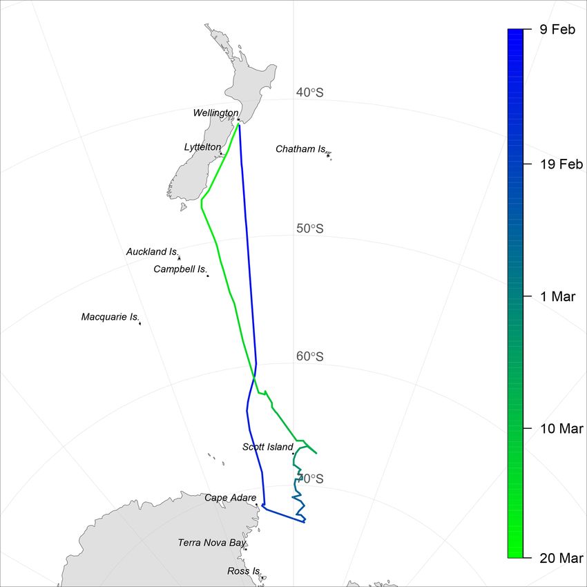
S. Kremser et al.: Measurements over the Southern Ocean 3119
Table 2. Table of instruments related to aerosol–cloud interactions that were deployed on the RV Tangaroa and are described in this study.
Instrument Type Location on the ship Parameter Section Research aim
AWS Automatic weather station Monkey island Pressure, temperature, 2.2 1
RH, wind
Eppley precision spectral Shortwave radiometer Monkey island Shortwave radiation 2.2 1
pyranometer (0.285 to 2.8 µm)
Eppley lab precision in- Downwelling infrared radiome- Monkey island Longwave radiation 2.2 1
frared radiometer ter (4 to 50 µm)
InterMet iMet-1-ABxn Radiosonde Fantail Pressure, temperature, 3.1.1 1&5
RH, wind, GPS
Windsond Radiosonde (ascent and de- Fantail pressure, temperature, 3.1.1 1&5
scent) RH, wind, GPS
Lufft CHM 15k Ceilometer Gilson gantry Attenuated backscatter, 3.2 1
CBH
Sigma Space MiniMPL Mini Micro Pulse Lidar Monkey island Attenuated backscatter, 3.3 1
CBH
Metek Micro Rain Radar Rain radar Port side of gallery Precipitation 3.4 1
Brinno BCC200 Sky camera Monkey island Sky images 3.5 1
Allskypi Sky camera Monkey island Sky images 3.5 1
Microtops-2 Sun Photometer Manual on deck AOD, water vapour, fine- 3.6 1, 2, & 3
and coarse-mode AOD at
500 nm
Picarro G2301 Cavity ring-down spectrometer Middle laboratory Atmospheric CO2 & 3.7 N/A∗
CH4
SwellPro Splash Drone 3 UAV Foredeck 0.38 to 17 µm, tempera- 3.1.2 2&5
ture, RH
Helikite Tethered balloon kite Fantail 0.38 to 17 µm, tempera- 3.1.3 2&5
ture, RH
Filter sampler Filter Bridge mezzanine Ice-nucleating particles 3.9 2&6
deck (front)
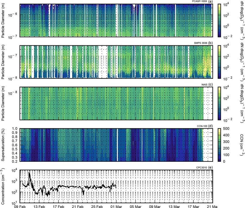
PCASP-100X Optical particle counter Container laboratory 0.1 µm < Dp < 3.0 µm 3.8.1 2, 3, & 6
CCN-100 Cloud condensation nuclei Container laboratory 0.2 % < s < 1.0 % 3.8.2 2, 3, & 6
counter
CPC3010 Condensation particle counter Container laboratory 0.01 µm < Dp < 3 µm 3.8.3 2&6
SMPS3936 Scanning mobility particle size Container laboratory 0.02 µm < Dp < 0.5 µm 3.8.4 2&6
spectrometer
NAIS Neutral cluster and air ion spec- Bottom of main mast 2 nm < Dp < 42 nm 3.8.5 2&6
trometer
GC-SCD Gas chromatograph – sulfur Container laboratory Dissolved DMS 3.10.1 4&6
chemiluminescent detector
MICA Mid-Infrared CAvity enhanced Middle laboratory Atmospheric and dis- 3.10.2 4&6
spectrometer solved OCS, CO2 , and
CO
RH – relative humidity; CBH – cloud base height; AOD – aerosol optical depth; CH4 – methane; DMS – dimethyl sulfide; OCS – carbonyl sulfide; CO – carbon monoxide.
∗ CO measurements were mainly used for contamination detection.
2
A pair of shortwave radiometers (0.285 to 2.8 µm – Epp- brated against salinity as determined from CTD (conductiv-
ley precision spectral pyranometer, PSP) and a second pair ity, temperature, and depth sensor) measurements and have
of downwelling infrared radiometers (4 to 50 µm – Eppley an estimated accuracy of 0.05 ‰. The “hull” temperature of
lab precision infrared radiometer, PIR) are installed on the the ship is measured by a remote SBE 38 thermometer (Sea-
ship. The pairing of the instruments enabled corrections to Bird Electronics) located close to a pumped seawater intake
the measurements to be made by accounting for shadow- near the bow, with a continuous flow to minimise heating
ing by the ship. Salinity was calculated using the SBE 21 artefacts and an expected accuracy of 0.2 ◦ C.
SeaCAT thermosalinograph (Sea-Bird Electronics Inc., WA, The meteorological measurements together with dissolved
USA) conductivity and temperature measurements. The in- DMS measurements (Sect. 3.10.1) were used as inputs
strument is installed as part of the underway seawater mea- to the National Oceanic and Atmospheric Administration
surement suite, with the surface water intake at a depth of (NOAA) Coupled Ocean–Atmosphere Response Experi-
about 7 m below the surface on the mid-port side of the ves- ment (COARE) meteorological and gas exchange algorithm
sel. The salinity measurements have been periodically cali- (Fairall et al., 2003, 2011; Blomquist et al., 2006) to de-
https://doi.org/10.5194/essd-13-3115-2021 Earth Syst. Sci. Data, 13, 3115–3153, 2021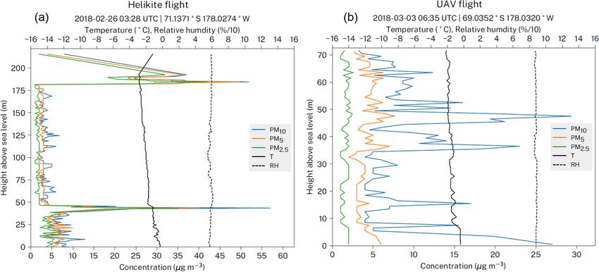
3120                                                                  S. Kremser et al.: Measurements over the Southern Ocean

Figure 2. Summary of the processing scheme of the meteorological measurements (pressure (P ), temperature (T ), relative humidity (rh),
wind (u), wind direction (wd), short- and longwave downwelling radiation (Sd, Ld)) from the AWS and radiometers measurements that were
stored in the Tangaroa data acquisition system. Wind corrected to 10 m (u10 ), heat flux (H ), and latent heat (λE) were derived from these
measurements and then, together with measured dissolved DMS concentrations, used to derived the sea–air fluxes of DMS.

rive meteorological values for standard reference heights               ibration procedures, which are also described below in the
(e.g. u10 ), energy and gas exchange coefficients, and sea–air          respective sections.
fluxes of DMS (Sect. 4.3.1).
   AWS measurements were complemented by human
weather observations, all-sky cameras, ceilometer, Mini Mi-             3.1     In situ measurements and remote sensing
cro Pulse Lidar (MiniMPL), and Micro Rain Radar measure-                        observations
ments, which provided important information about visibil-              3.1.1    Radiosondes
ity, sky conditions, clouds, cloud type, and the amount of pre-
cipitation or fog events. In addition, up to three daily regular        Radiosondes are balloon-borne instruments that measure the
radiosondes of type InterMet iMet-1-ABxn were launched                  vertical profile of temperature, relative humidity, and pres-
throughout the voyage, as well as smaller balloons carry-               sure. Altitude, wind direction, and wind speed are calculated
ing Windsond radiosondes that were launched in synopti-                 from the GPS location of the sonde. A total of 58 radiosondes
cally interesting conditions, e.g. within low pressure systems          of type InterMet iMet-1-ABxn (hereafter referred to as iMet)
(Sect. 3.1.1). An overview of all radiosonde releases during            and 12 of type Windsond were released on a weather bal-
the voyage is provided in Tables B1 and B2.                             loon during the voyage (see Tables B1 and B2). The iMet ra-
   All meteorological data are available in NetCDF format at            diosondes were attached to 100 g Kaymont weather balloons
UTC time and are provided with the data set accompanying                and released two to three times per day at about 07:30, 00:00,
this study. Section 4.1 below provides some detail about the            and 19:30 UTC. The typical height reached by the balloons
meteorological conditions encountered during the voyage.                was between 10 and 20 km a.s.l. Of the total iMet radioson-
                                                                        des released, one failed right after launch, and one failed at
                                                                        216 m a.s.l. In addition, two iMet radiosondes had faulty or
                                                                        intermittent relative humidity readings. No iMet radiosondes
3   Instrument descriptions                                             were released north of 58◦ S or in unsuitable weather condi-
                                                                        tions, e.g. when wind speed was exceeding 35 kn or in high
In addition to the instrumentation mentioned above, atmo-               swell. In addition to the iMet radiosondes, S1H3 Windsond
spheric measurements were conducted using a range of in-                radiosondes were launched sporadically throughout the voy-
struments, including a cavity ring-down spectrometer, cloud             age. The typical altitude reached by the Windsond radioson-
condensation nuclei counter, condensation particle counter,             des was 6 km. In total, five of the Windsond devices were
mobility particle size spectrometer, optical particle counter,          equipped with a second balloon to perform measurements
neutral cluster and air ion spectrometer, a filter sampler, teth-       during the descent, but only two descending profiles were
ered balloon, and an unmanned aerial vehicle (UAV). Dur-                successfully measured.
ing rare clear-sky conditions, aerosol optical depth (AOD)                 The iMet radiosondes communicated with the base station
measurements were made using a hand-held Sun photometer.                by radio at 403 MHz and included a pressure sensor with an
The instrumentation and measurement techniques of each in-              accuracy of 0.5 hPa and a resolution of < 0.01 hPa. As de-
strument are described below. Furthermore, all data sets de-            scribed by the manufacturer, a thermistor was used to mea-
scribed here include some means of quality control and cal-             sure the temperature with an accuracy of 0.2 ◦ C and a resolu-

Earth Syst. Sci. Data, 13, 3115–3153, 2021                                               https://doi.org/10.5194/essd-13-3115-2021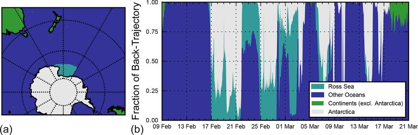
S. Kremser et al.: Measurements over the Southern Ocean                                                                     3121

tion of ±0.01 ◦ C and a capacitive polymer sensor measuring           While the expected battery lifetime of the UAV was
relative humidity with an accuracy of ±5 % and a resolution       15 min, this was reduced to 6 min due to the low atmo-
of < 0.1 %. The temporal resolution of the iMet sonde mea-        spheric temperature, resulting in a lower-than-expected al-
surements is about 30 s, with a vertical resolution of about      titude reached and unplanned landing on the ocean surface.
60 m, except during periods of poor signal reception, which       After the battery regained enough power to take off again,
can decrease the temporal and vertical resolution.                the UAV was recovered. Measurements of aerosol concen-
   The lightweight (about 12 g), low-operating-cost Wind-         tration, temperature, pressure, and humidity were recorded
sond radiosonde provides real-time wind, temperature, and         up to an altitude of about 70 m. No measurements were re-
relative humidity profiles in the lower part of the troposphere   trieved from the second UAV flight due to a faulty assembly
with an operational ceiling of 9 km a.s.l. The system has an      of the propellers, which resulted in the loss of the aircraft.
operational radio frequency configurable in the range of 400          While the operator had about 7 flight hours of experience
to 480 MHz. The Windsond uses a band-gap temperature              with the UAV, which is sufficient to obtain a UAV pilot cer-
sensor with a measurement range between −40 and +80 ◦ C,          tification in New Zealand, the conditions were challenging,
an accuracy of 0.2 ◦ C, and a resolution of ±0.01 ◦ C. Relative   so more experience, e.g. flight hours and practice in operat-
humidity was measured using a film capacitor sensor with          ing the UAV safely around obstacles, would have helped to
high accuracy (±1.8 %) and a resolution of 0.05 %. Pres-          mitigate some of the risks.
sure was measured directly using a microelectromechanical
piezoresistor pressure sensor with an accuracy of 1 hPa and       3.1.3    Helikite
a resolution of 0.02 hPa. The Windsond GPS ground station
was not equipped with a GPS receiver; therefore, latitude and     Similar to the UAV flights, two Helikite flights were con-
longitude were determined using an on-board GPS receiver          ducted in suitable weather conditions subject to wind speed
pseudorange without differential correction. Wind speed and       of below 5 m s−1 . For the first flight, the Helikite was
direction is determined independently from latitude and lon-      equipped with an iMet radiosonde and an OPC-N2, provid-
gitude using the GPS signal; wind speed accuracy is about         ing profiles of aerosol concentration, as well as temperature,
5 %. The accuracy of the wind direction depends on the GPS        pressure, and humidity profiles. The second Helikite flight
conditions and is therefore determined by the accuracy of the     had to be terminated shortly after launch as the weather con-
GPS sensor.                                                       ditions changed rapidly, resulting in no measurements.
                                                                     The Helikite comprised a large 6 m3 balloon with a sturdy
3.1.2   Unmanned aerial vehicle – UAV
                                                                  kite base. Lift can be achieved by inflating the balloon with
                                                                  helium and is aided by the additional lift of the kite. As a re-
During the voyage, two UAV flights were performed when            sult of the large volume of the balloon, the total payload can
the observed wind speed was below 5 m s−1 . For the first         be around 2 to 3 kg. The Helikite was flown off the fantail and
flight, which took place on 4 March 2018, the UAV was             was anchored to an electric winch fitted with > 1 km of high
equipped with an optical particle counter (OPC) of type Al-       tensile strength Dyneema line. This system itself offers the
phasense OPC-N2, a GoPro Hero4 camera, and a customised           opportunity to fly more expensive sampling equipment than
radiosonde. The radiosonde was equipped with a SHT75              typically deployed during a radiosonde flight where equip-
temperature and relative humidity sensor. Temperature can         ment is usually not recovered.
be measured between −40 and +40 ◦ C with an accuracy of              The first flight of the Helikite occurred midway through
0.3 ◦ C and a resolution of ±0.01 ◦ C and relative humidity       the voyage on 26 February 2018. Conditions were good, with
can be measured with an accuracy of 1.8 % and a resolu-           wind speeds less than 5 m s−1 . Due to the inexperience of
tion of 0.05 %. A customised radiosonde was required to be        the Helikite operator, the Helikite was flown in near neutral
deployed on the UAV (rather than using a standard sonde),         buoyancy; i.e. the lift provided by the balloon was near or
as it needed to interface with the OPC-N2 sensor and data         equal to the weight of the payload. As a result, the only lift
had to be transferred over radio to the ground station. The       received during the flight was from the kite alone. Once the
Alphasense OPC-N2 is an OPC designed to count ambient             Helikite left the slipstream of the Tangaroa, it rose slowly to
particulate- and drizzle-sized cloud droplets between 0.38–       an altitude of 260 m. At this stage, the additional weight of
17 µm in size. Ambient air is drawn into the sensor by a          the tethered string counter-balanced all lift. After sampling
small rotary micro-fan at a flow rate of about 1.2 L min−1 .      for around 45 min, the system was reeled back in.
The air enters the front of the device through a 6 mm ori-
fice into an open optical cavity, where red laser light (around   3.2     Ceilometer
650 nm) is incident on the incoming aerosol. Scattered light
from the aerosol is collected via an elliptical mirror and a      During the voyage a ceilometer, which is a low-power li-
dual-element photodetector. These measurements are used to        dar, made continuous measurements of the overlying atmo-
determine the particle size and particle number concentra-        spheric state. The ceilometer deployed on the voyage was a
tion.                                                             Lufft CHM 15k, which operated at an infrared wavelength

https://doi.org/10.5194/essd-13-3115-2021                                         Earth Syst. Sci. Data, 13, 3115–3153, 2021
3122                                                               S. Kremser et al.: Measurements over the Southern Ocean

of 1064 nm, with a maximum range of 15 km. The ceilome-             the environmental enclosure containing the lidar to provide
ter was installed on the Gilson gantry behind the monkey is-        variable-angle scanning throughout the voyage. Azimuth was
land (Fig. 3), located approximately 16 m a.s.l. The ceilome-       fixed for observations (pointing outward from the side of
ter continually emits short light pulses vertically into the at-    the ship) and the scanning head was programmed with an
mosphere, where light is scattered back by clouds, aerosol,         elevation-only scanning routine that included the following
and air molecules. By detecting the runtime of the return sig-      angles: 0, 5, 10, 15, 20, 30, 40, 45, 50, 60, 70, 80, and 90◦ ele-
nal, the ceilometer identifies the lowest altitude of a cloud       vation. The finer 5◦ elevation step was used near the horizon,
as the layer with higher particle backscatter characteristics.      and then 10◦ steps from 20 to 90◦ (zenith). An observation
The backscatter is calculated at 1024 vertical levels in the        was also made at 45◦ because it is convenient geometrically.
atmosphere (about 15 m vertical resolution). By applying            At 0 and 90◦ , the observations were 12 min long, at other an-
detection algorithms using the operational software to the          gles 6 min, resulting in the full scanning cycle taking 90 min.
backscatter measurements, quantitative information on cloud         The elevation angle of each particular observation is recorded
base height (CBH), cloud fraction (CF), cloud layers, and           in the data file. Note that there were some instances during
boundary layer height can be determined. As the emitted sig-        the campaign (overall 9 d) when a software failure caused the
nal is strongly attenuated by thick clouds, it is often not pos-    scanning system to not follow the programmed schedule.
sible to observe the middle or tops of clouds. On some occa-           The MiniMPL was not motion stabilised on the ship, and
sions, the movements of the ship (pitch and roll) affected the      so any ship movement is captured within each integration pe-
ceilometer measurements when there were horizontally in-            riod of the measurements. While each individual laser pulse
homogeneous clouds, producing a vertical filament structure         will be received near instantaneously and “freeze” the ship
in the backscatter.                                                 motion, the full number of pulses, i.e. scans, during the
                                                                    minute-long integration period will result in a number of
3.3    Sigma Space MiniMPL
                                                                    profiles over a range of pointing angles due to ship motion,
                                                                    which will be all averaged together for that minute. This ap-
The MiniMPL is a sophisticated laser remote sensing sys-            plies for the vertical-pointing scans and the scans done at the
tem that provides continuous, unattended monitoring of the          distinct elevation angles.
profiles and optical properties of clouds and aerosols in              The instrument produces native binary files (“mpl”) with
the atmosphere. A micropulse lidar (MPL) transmits laser            backscatter and housekeeping metadata, which can be con-
pulses that scatter (reflect) off particles in the atmosphere.      verted to NetCDF files using manufacturer supplied soft-
The MPL then measures the intensity of backscattered light          ware (SigmaMPL) or third-party software (mpl2nc). The pri-
using photon-counting detectors and transforms the signal           mary output quantity is the normalised relative backscatter
into atmospheric information in real time. During the cam-          (NRB) profile, representing the backscattering of light (in
paign, aerosol backscatter data were collected using the            photon counts km2 µs−1 µJ), after correcting and normalis-
Sigma Space MiniMPL, which is a compact version of the              ing the measurements. An auxiliary GPS unit was connected
standard MPL described by Ware et al. (2016). The man-              to the lidar, whose output was recorded in the product files.
ufacturer specification for the MiniMPL’s maximum range             The instrument was installed on the monkey island (Fig. 3).
is 30 km. However, accurate MPL measurements can rarely                The instrument ordinarily requires range-dependent cali-
be obtained up to this height. This is because the retrievals       bration of backscatter in the form of dead time, overlap, and
are strongly impacted by absorption and scattering along            afterpulse corrections, which account for the saturation of the
the beam path, with the signal-to-noise ratio decreasing with       photon counter, incomplete overlap of the outbound and in-
height, resulting in a lower effective range. During the cam-       bound beams, and post-pulse reflections from the internal
paign, this range was mostly limited to the first few kilome-       parts of the instrument, respectively. These were supplied
tres due to dense low-level clouds that saturated the return        by the manufacturer. An improved calibration was produced
signal. Other periods of clearer skies had distinct cloud fea-      post-voyage, which addresses a technical issue with the man-
tures at up to 8–9 km before fading into background noise           ufacturer calibration (bit truncation of dead time polynomial
above these features. Our data processing was limited to            coefficients) and a change in overlap which might have hap-
10 km, as the voyage focused on marine boundary layer               pened during transport and deployment of the instrument.
clouds as well as low- and middle-level clouds as defined           The data product produced with the third-party mpl2nc soft-
in research aim 1.                                                  ware was calibrated with the improved calibration and is sup-
   The MiniMPL is a dual-polarisation micropulse lidar op-          plied with the data set.
erating at a wavelength of 532 nm at 2.5 kHz (pulse energy             The CHM 15k ceilometer and Sigma Space MiniMPL
is 3–4 µJ). Laser light that is scattered back towards the in-      measurements were both processed using the Automatic Li-
strument is collected by an 80 mm diameter receiver (Spin-          dar and Ceilometer Framework (ALCF, Kuma et al., 2021a).
hirne et al., 1995; Campbell et al., 2002; Flynn et al., 2007).     While ALCF was developed to provide a tool to evaluate
The vertical range resolution was set at 15 m during the ship       clouds simulated by climate models or reanalysis data us-
campaign. A two-axis scanning head was mounted on top of            ing ceilometer or MiniMPL observations, ALCF can be run

Earth Syst. Sci. Data, 13, 3115–3153, 2021                                           https://doi.org/10.5194/essd-13-3115-2021
S. Kremser et al.: Measurements over the Southern Ocean                                                                     3123

Figure 3. A diagram showing the locations of the atmospheric measurement equipment aboard RV Tangaroa. A line pump for the common
aerosol inlet was used to pump sample air from above the bridge to the aerosol container lab.

independently of any model input to process ceilometer or          3.4   Micro Rain Radar
MiniMPL observations. ALCF can ingest the raw measure-
ments, transform backscatter profiles to profiles comparable       During the voyage a Metek Micro Rain Radar 2 (MRR-
with different instruments, and output the results in NetCDF       2) made continuous measurements of the overlying at-
format. ALCF is described in detail in Kuma et al. (2021a).        mospheric state between 7 and 27 February 2018.
   Two different data products are provided for both the           The MRR-2 is a vertical-pointing FM-CW (frequency-
ceilometer and MiniMPL data, level 0 and level 1:                  modulated continuous-wave) radar with a centre frequency
                                                                   of 24.23 GHz and a frequency modulation between 0.5–
  – Ceilometer level 0 contains one file per 5 min of ob-          15 MHz. The scatter return signal can be processed to derive
    servations in the native NetCDF format (.nc files). The        Doppler spectra at a number of predefined vertical ranges,
    5 min files provide one profile every 2 s, with a temporal     from the ground to several hundred metres. For rain droplets,
    resolution of 15 m.                                            the relationship between terminal fall velocity and drop di-
                                                                   ameter is used to derive vertical profiles of the rain drop
  – MiniMPL level 0 contains one file per hour of obser-           size distribution from the Doppler spectra. These drop size
    vations in the native binary (.mpl) format which can           distributions can be integrated to derive rain rates even for
    be processed using the proprietary SigmaMPL software           very small amounts of precipitation, below the thresholds
    or converted to NetCDF format using a Python tool              detectable by conventional rain gauges. The software sup-
    (mpl2nc). The hourly files provide one profile every 6 s       plied by the manufacturer completes all this processing and
    with a vertical resolution of 15 m.                            also makes estimates of other parameters, such as liquid wa-
                                                                   ter content. The temporal resolution of the measurements
  – MiniMPL (minimpl_mpl2nc) contains MiniMPL data                 is 10 s. Measurements of snowfall using this instrument are
    that were processed using the mpl2nc source code to            more challenging because the particle backscattering cross
    convert raw MiniMPL data files to NetCDF files. The            sections depend on both their mass and shape, while termi-
    hourly files provide one profile every 6 s with a vertical     nal velocities relationship to particle size depends on their
    resolution of 15 m.                                            projected area. In the case of snowfall, we use the method
                                                                   of Maahn and Kollias (2012) to process the raw data to de-
  – Level 1 contains ALCF-processed raw ceilometer and             rive radar reflectivity, velocity, spectral width, and snowfall
    MiniMPL data sets (one file per day) in NetCDF for-            rate estimates. The radar was installed on the port side of the
    mat. The data products included are time series of verti-      gallery beneath the bridge (Fig. 3).
    cal backscatter profiles, backscatter standard deviation,         It should be noted that the Doppler velocity information is
    cloud base height, cloud mask, and lidar ratio. The data       integrated over a period, meaning that variations in the ship
    were subsampled to 5 min intervals with a vertical reso-       motion will impact the spectral width of the signal, adding
    lution of 50 m.                                                additional uncertainty to the derived MRR precipitation data.

https://doi.org/10.5194/essd-13-3115-2021                                         Earth Syst. Sci. Data, 13, 3115–3153, 2021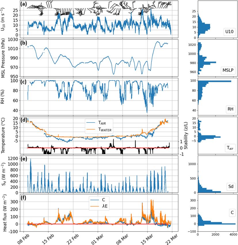
3124                                                               S. Kremser et al.: Measurements over the Southern Ocean

There are also signs of the Doppler velocity being degraded         Microtops-2 Sun photometer, operating at five wavelengths.
by ship motion around 22:00 UTC. Unfortunately, disdrom-            The instrument was calibrated prior to the voyage by NASA
eter measurements were not available on this voyage, and            and operated according to the Aerosol Robotic Network
therefore the MRR was not calibrated. This also potentially         (AERONET) Maritime Aerosol Network (MAN) protocols
adds uncertainty to the derived precipitation values when us-       with an attached GPS receiver to log positional information.
ing these data quantitatively. However, the data are still very     Scans were usually taken in groups of five measurements
valuable for masking periods of precipitation as used and de-       and only made under clear-sky conditions with no clouds
scribed in Hartery et al. (2020a).                                  present near or around the Sun, taking care to avoid mea-
                                                                    surements through cirrus clouds. Clear-sky conditions were
3.5    Sky cameras
                                                                    rare and only observed for less than 2 % of the time. Due
                                                                    to the otherwise high cloud cover occurrence during the voy-
A pair of Brinno BCC200 cameras were installed on the star-         age (see Fig. 11 below), these measurements were performed
board and port side of the monkey island (Fig. 3). The cam-         only four times on three distinct days. Processed products in-
eras were configured to capture an image of the sky every           clude AOD at five wavelengths, water vapour content, the
5 min. The resolution of the images is 1280 × 720 pixels,           Ångström parameter and aerosol optical depth for the fine
and they are recorded in a video file (Motion JPEG). These          (submicron) and coarse (supermicron) modes calculated ac-
images are complementary to the human weather observa-              cording to the spectral deconvolution algorithm of O’Neill
tions, ceilometer, and lidar data to evaluate cloud cover, cloud    et al. (2003). The data are available via the MAN website
types, and cloud base height during the voyage. An additional       for the TAN1802 voyage (2020). To date, over 600 voyages,
camera system, named allskypi, was also installed on the            including the TAN1802 voyage described here, have con-
monkey island, adjacent to the MiniMPL. The allskypi sys-           tributed to the MAN database providing a valuable global re-
tem contained a ZWO ASI178MC (3096×2080 pixels) cam-                source for analyses (e.g. Smirnov et al., 2009, 2011) and use
era with a fisheye lens connected to a Raspberry Pi single-         in validation and model development of important aerosol
board computer. Allskypi acquired images at seven expo-             components such as oceanic sea salt (Bian et al., 2019).
sure levels every 5 min, which, in post-voyage processing,
were combined into a single image by exposure fusion as de-         3.7   Cavity ring-down spectrometer – Picarro
scribed in Mertens et al. (2009). Over the course of the voy-
age, over 60 000 images were taken, resulting in nearly 9000        By the voyages nature, the ship did not always head into the
HDR images. When combined with ship positioning data,               wind. As a result, there were distinct times throughout the
including roll and pitch, cloud fraction can be determined          voyage when winds from the stern outpaced the motion of the
by simple thresholding techniques such as the ELIFAN al-            ship, and therefore the sampling line of air sampling instru-
gorithm presented in Lothon et al. (2019). This algorithm           ments was often exposed to exhaust from the ship. This prob-
was adapted to the allskypi system to obtain cloud fractions        lem was largely unavoidable, but the ship’s measurements
by masking out pixels below an elevation of 20◦ to exclude          of wind speed and heading combined with high-precision
ship structure and to avoid low elevation angles that thresh-       measurements of carbon dioxide (CO2 ) were used to iden-
olding techniques struggle to accurately resolve. Additional        tify contamination episodes. Experience from previous voy-
masks were also applied for the remaining ship structure and        ages (e.g. Law et al., 2017) has shown that the cavity ring-
for the solar disc. Furthermore, a record of whether or not         down spectrometer (CRDS) is ideally suited to detect ship
the Sun was obscured by clouds was produced by monitor-             exhaust contamination. For this and other reasons beyond
ing the image saturation over the solar disc. All-sky imagery,      the scope of this paper, a CRDS (G2301, Picarro) was in-
along with estimates of cloud fraction and Sun obscuration          stalled on the ship and operated continuously throughout the
obtained during this voyage, was primarily used for quality         voyage. The CRDS was installed in an equipment room off
assurance and quality control (QA/QC) of other sky-viewing          the middle lab (Fig. 3) measuring atmospheric mixing ra-
observations such as the ceilometer and MiniMPL measure-            tios of CO2 and methane (CH4 ) continuously at 1 Hz. Air
ments (as described in, e.g. Wagner and Kleiss, 2016). Cloud        for analysis by the CRDS was obtained from an inlet on the
fraction derived from the sky camera product is also useful         forward light tower above the bridge (∼ 20 m a.s.l.) via an
for model evaluation, and when combined with the raw im-            airline to the middle lab. Air was pumped down from the air-
agery and ceilometer data it could potentially be used to clas-     line at about 2 L min−1 , of which 150 mL min−1 (determined
sify cloud types as described in Huertas-Tato et al. (2017).        by a mass flow controller) is used for analysis. Before the air
                                                                    from the airline was sampled by the analyser, it was dried
3.6    AERONET Maritime Aerosol Network (MAN)
                                                                    to a dew point of 2–4 ◦ C using a thermoelectric cooler and
       hand-held Sun photometer
                                                                    then dried further to a dew point between −30 and −40 ◦ C
                                                                    using a back-flushed Nafion dryer in which remaining wa-
When clear-sky conditions were present, column aerosol              ter vapour in the air is transferred to the CRDS exhaust air
measurements were made using a portable Sun-pointing                that had been dried by passing it through a molecular sieve

Earth Syst. Sci. Data, 13, 3115–3153, 2021                                          https://doi.org/10.5194/essd-13-3115-2021
S. Kremser et al.: Measurements over the Southern Ocean 3125
trap. While the Picarro instrument does measure the concen- Air sampled from the sampling line connecting the CCN,
tration of water vapour in the air, in this system, the water SMPS, and CPC was dried with a custom-built diffusion drier
vapour measurement was only used as a diagnostic indicator prior to being sampled by each instrument. The inlet of the
of system performance. Solenoid valves controlled by the Pi- sampling line for the PCASP-100X was also positioned in
carro were used to select either pre-dried air for analysis, or the stream of the sampling conduit to improve sampling ef-
air from one of three reference tanks, plus a target tank, for ficiency of particulate. The PCASP-100X used on the ship
system calibration. A calibration sequence was automatically was an airborne version designed to be isokinetic for an in-
run twice per day. strument inlet speed of about 100 m s−1 with the instrument
The analyser has a built-in Windows 7 PC for data ac- mounted external to the aircraft on a pylon. For operating
quisition and control of the CRDS system. Measurements the instrument in the laboratory, airflow was drawn through
were stored in the form of hourly text files on the Picarro the instrument inlet with an external ring compressor purge
PC’s solid-state drive. File times are in UTC, whereas the Pi- pump, which improved response time and isokinetic sam-
carro’s internal PC was set to New Zealand Standard Time pling efficiency of the PCASP by increasing the airflow in
(NZST) (UTC + 12 h) and was synchronised to Tangaroa’s the region of the internal cavity hypodermic inlet. However,
time server. Picarro’s sample time is around 1 s (there is some the air sampled by the PCASP was not dried. The temper-
variability around this value), but this is shared among the ature within the aerosol container laboratory was typically
three compounds measured (CO2 , CH4 , and H2 O), so the in- about 20 ◦ C, while the ambient temperature was about 0 ◦ C
dividual compound sample time is around 3 s. Once per day, between 15 February and 15 March. As such, the relative
the data files were backed up to the network drives of the humidity of the air sampled by the PCASP was likely sub-
ship and processed to produce diagnostic plots to check sys- stantially lower than the ambient relative humidity. The dif-
tem operation and performance. ference between the laboratory and ambient relative humid-
One NetCDF file containing the level 1 data product of the ity would have partially dried the particles; though, this has
Picarro measurements is provided, containing 5 min average not been explicitly quantified or accounted for in the data as
of the CO2 and CH4 concentrations measured during the voy- it would require a priori knowledge of particle composition
age. Data quality flags are provided for every substance, in- and hygroscopicity. As a result, there are potentially biases
cluding flags to mark data subject to exhaust contamination. between the size of particles detected by the PCASP and par-
ticles detected by the SMPS. These biases are likely greater
3.8 Common aerosol sampling conduit
outside the period of 15 February to 15 March as a result of
there being a smaller difference in temperature between the
Throughout the voyage, the container laboratory, which laboratory and ambient conditions. Finally, the remainder of
housed the majority of the underway aerosol sampling in- the air passing through the main sampling conduit was di-
strumentation, was positioned behind the mid-ship exhaust rected towards the exhaust via the main pump. A schematic
(2 m a.s.l.). To prevent exhaust air from contaminating the layout of the plumbing is represented in Fig. 4.
in situ measurements of ambient marine aerosol, ambient In addition, a Neutral cluster and Air Ion Spectrometer
air was drawn from the mast of the RV Tangaroa, through (NAIS) was installed on at the bottom of the top platform
the conduit (Fig. 3) to the container laboratory, at a rate of of the ship. All of these instruments will be described in fur-
4.1 × 10⁻² m3 s−1 . Size-dependent losses of particulate to ther detail below. Operation of different types of instruments
conduit walls from an isokinetic sampling, gravity, turbu- covering overlapping, or often the same, particle size ranges
lence, and diffusion are described in detail in Hartery et al. offers a measure of mutual quality control on the measure-
(2020b). The average transit time for particulates through the ments.
40 m long common aerosol sampling conduit was < 8 s. The
inlet of the conduit was angled downwards to prevent the ac-
cumulation of precipitation within the inlet region. 3.8.1 Optical particle counter
The aerosol container laboratory (Fig. 4) was equipped
with the following instruments: an optical particle counter of The abundance of particles in the size range 0.1–3.0 µm
type PCASP-100X, a cloud condensation nuclei counter of was measured with a passive cavity aerosol spectrometer
type CCN-100, a condensation particle counter of type CPC- probe (PCASP-100X; Droplet Measurement Technologies).
3010, and a scanning mobility particle sizer (SMPS). Within The PCASP and SMPS (see Sect. 3.8.4) are both spectral
the aerosol laboratory, the main sampling conduit connected particle counters which provide the partial number concen-
to a plumbing manifold with three outflows: (1) a sample tration at given sizes, i.e. the number of particles observed
flow for the CCN-100, SMPS3936, and CPC3010; (2) a sam- within various subranges over the total range of observable
ple flow for the PCASP-100X; and (3) a primary exhaust flow sizes. PCASP measures size according to the optical diame-
(Fig. 4). The inlet of the sampling line for the CCN, SMPS, ter (i.e. how it refracts and scatters light). The advantage of
and CPC was positioned within the stream of the main sam- the PCASP is that it can record data quickly (1 Hz), while
pling conduit to improve sampling efficiency of particulate. the SMPS instrument is slow. However, the disadvantage of
https://doi.org/10.5194/essd-13-3115-2021 Earth Syst. Sci. Data, 13, 3115–3153, 20213126 S. Kremser et al.: Measurements over the Southern Ocean
Figure 4. A schematic layout of the particle counting instruments in the aerosol container laboratory (not to scale).
the PCASP is that it can only measure particles larger than concentration. However, if the standard deviation of the
100 nm. 1 Hz subsamples was more than 3 times greater than the
The PCASP instrument recorded the number of observed square root of the concentration, then the 5 min sam-
particles in 30 particle size bins at a frequency of 1 Hz. While ple was discarded. This additional measure removed
the PCASP measurement frequency is high, it is generally 184 samples.
beneficial to integrate the PCASP over a period as long as
5 min to get better counting statistics and decrease the rela- 4. The final measure involved removing observations in
tive measurement uncertainty. As a result, the measurements the first size bin, as the lower threshold of particle de-
in each size bin were block-averaged into 5 min intervals in tection in this bin is not well defined due to potential
a post-processing stage. Between 9 February and 21 March variations in the refractive index of the measured parti-
2018, there were a total of 12 000 5 min intervals, through- cle(s). Additionally, the fourth and fifth size bins were
out which the instrument recorded for a total of 11 400 inter- added together and redefined as a single bin, as the fifth
vals. Four additional measures of quality control were imple- size bin was in between linear gain stages of the particle
mented in the data post-processing chain. counter, which led to spuriously low counts.
1. The first measure involved using the mole fraction of Overall, 81.7 % of the measurements taken remained af-
CO2 in a coincident sampling line, measured by the Pi- ter the post-processing described above. This is a reason-
carro instrument, to screen the 1 Hz subsamples for con- able data retention rate, considering the challenges of sam-
tamination by ship exhaust (Hartery et al., 2020b). For pling just about 10 m ahead of the mid-ship exhaust. After
11 118 of the 5 min intervals with data, the mole frac- post-processing of the measurements, the processed particle
tion of CO2 was less than 405 ppm and the sample was size spectra were corrected to standard temperature and pres-
flagged as “clean air”. sure. In addition, the particle size spectra were corrected ac-
cording to parameterisations of the sampling and transport
2. The second measure involved using the relative wind efficiency of aerosol particles detailed in Brockman (2001).
direction measured by the sonic anemometers in a sim- These calculations accounted for anisokinetic sampling con-
ple wind sector analysis. Measurements that were taken ditions, diffusion, gravitational settling, and turbulence. Fi-
when the relative wind direction from both the port nally, the total particle concentrations in each size bin were
and starboard anemometers were within 60◦ aftward normalised by the logarithm of the bin’s width.
were removed. All other samples were flagged as having
come from a “clean sector”. Out of the 11 118 clean air 3.8.2 Cloud condensation nuclei counter
samples (i.e. not contaminated by ship exhaust), 9986
were from clean sectors. The concentration of individual particles that can form into
cloud droplets, i.e. cloud condensation nuclei (CCN), was
3. The third measure involved calculating the standard de- measured at varying water vapour supersaturations with a
viation of the 1 Hz subsamples within each of the 5 min CCN counter (CCN-100; Droplet Measurement Technolo-
intervals (Hartery et al., 2020b). Even for a steady con- gies). The CCN and condensation particle counter (see
centration of particles, the number of particles counted Sect. 3.8.3) instruments are integrating particle counters,
within a given interval will vary according to Poisson which provide the total concentration over a given size range.
counting statistics; thus, the standard deviation of the For a CCN-100 counter, the lower size threshold of observ-
1 Hz samples within the 5 min interval should be ap- able particles is dependent on the chamber supersaturation
proximately equal to the square root of the measured and the hygroscopicity of aerosol. The benefit of the CCN-
Earth Syst. Sci. Data, 13, 3115–3153, 2021 https://doi.org/10.5194/essd-13-3115-2021You can also read