Speciation based firefly algorithm for optimization in dynamic environments
←
→
Page content transcription
If your browser does not render page correctly, please read the page content below
Speciation based firefly algorithm for optimization in
                    dynamic environments

                               Babak Nasiri1 and M.R. Meybodi2
          1
              1Department of Computer Engineering and Information Technology
                   Islamic Azad University, Qazvin Branch, Qazvin, Iran
                                 nasiri.babak@qiau.ac.ir
           2
               Department of Computer Engineering and Information Technology
                      Amirkabir University of Technology, Tehran, Iran
                                   mmeybodi@aut.ac.ir

                                              ABSTRACT

        In many optimization problems in real world, objective function, design variable or con-
      straints can be changed during time, so optimal value of these problems also can be
      changed. These kinds of problems are called dynamic. Algorithms which are designed
      for optimizing in these environments have some principles that distinguish them from algo-
      rithms designed in static environment. In this paper, for the first time, an algorithm based on
      firefly algorithm is proposed for optimization in dynamic environment. Firefly algorithm is a
      new meta-heuristic algorithm with a great potential for discovering multiple optima simulta-
      neously. Mentioned ability of this algorithm has been used to propose a novel approach for
      multi-modal optimization in dynamic environments. The proposed approach evaluated on
      Moving peaks benchmark problem, which is the most famous benchmark for assessment in
      dynamic environments. The obtained results show the proper accuracy and convergence
      rate for the proposed approach in comparison with other well-known approaches.

      Keywords: Dynamic optimization problem, local search, Firefly Algorithm, Moving peaks
      benchmark.

1 Introduction

  In real world, many optimization problems are non-stationary and dynamic. These optimiza-
tion problems alter when the environment changes over time. Solving this type of problems by
algorithms designed specifically for static environment is almost disappointing. Finding global
optimal value is not sufficient for optimizing in dynamic environments and tracking optimum
during the changes in the environment is also important. During recent years, different groups
of methods have been proposed for solving optimization problems in dynamic environment.
Among them, evolutionary computing and swarm intelligence methods have received signifi-
cant attention during last decade. In order to design swarm intelligence algorithms for dynamic
environments, two important points have to be taken into consideration: outdated memory and
losing diversity.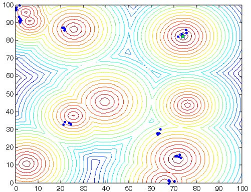
Outdated memory refers to condition in which memory of the components of the algorithm
may no longer be valid after a change in the environment. It can be solved by re-evaluating the
memory or forgetting it. Furthermore, losing Diversity happens due to nature of evolutionary
algorithms and swarm intelligence ones in converging to a point during executing the algo-
rithm. At this point, if a change happens in environment, converging to a new optimal point is
impossible or time consuming due to diversity loss. There are various methods for generating
or maintaining diversity in environment that will be discussed in following.

  The simplest way to react against environment change is to considering any changes as an
input of a new optimization problem which has to be resolved. In case of having enough time,
this solution is a proper option, but this time is often rather short for re-optimization. An attempt
to improve the optimization process and convergence rate is moving information of search
space from current environment to the next environment. If the change is extensive and there
is a little similarity before and after a change in the environment, restarting the optimization
algorithm can be the only proper option and any new use of collected information based on
problem space before the change will be misleading. In most of real world problems, intensity
of changes is not too much and new environment is closely related to the old environment.

  There are two approaches to deal with losing diversity. In the first approach, a diversity
maintenance mechanism runs during executing the algorithm (Hu and Eberhart, 2002). In
the second approach, diversity is always monitored, and as soon as it falls below a thresh-
old, the swarm will be re-diversified. Reported mechanisms in the literatures for either diver-
sity maintenance or re-diversification have been classified into four groups (Blackwell, 2007):
randomization (Hu and Eberhart, 2002), repulsion (Blackwell, 2003) (Blackwell and Branke,
2004), dynamic topology (Janson and Middendorf, 2004) and multi-populations (Blackwell and
Branke, 2004) (Blackwell and Branke, 2006) (Li, Branke and Blackwell, 2006) (Parrott and
Li, 2006) (Lung and Dumitrescu, 2007) (Blackwell, Branke and Li, 2008) (Du and Li, 2008) (Li
and Yang, 2009) (Liu, Yang and Wang, 2010). Hu and Eberhart proposed randomization to ran-
domize various proportions of the swarm to maintain some degree of diversity in order to track
better the optimum after a change. However, this approach may suffer from losing some use-
ful information due to randomization. Repulsion is used to repel the particles from each other.
Blackwell and Bentley proposed a repulsion mechanism by using the concept of atom in nature
and concluded that some charged particles which repel each other and orbit a neutral particle.
Dynamic topology prevents the convergence of particles to the global best position by changing
the topology of sharing information, thereby enhancing population diversity. Li and Dam pro-
posed grid-like neighborhood structure (Kennedy and Mendes, 2002). Janson and Middendorf
proposed HPSO, a tree-like structure hierarchical PSO (Janson and Middendorf, 2004), and
Hashemi and Meybodi Proposed CellularPSO, a hybrid model of particle swarm optimization
and cellular automata (Hashemi and Meybodi, 2009). In cellular PSO, a cellular automaton is
embedded into the search space and partitions the search space into some cells. In each cell,
a group of particles present and search for an optimum. Multi-population group is the most
used and promising group for optimizing in dynamic environment. Multi-population approach
divides the particles into some sub-swarms which each sub-swarm is responsible for searching
in a different area. Therefore, in multi-swarm approaches, each swarm searches for a local op-
timum and at the same time avoids overlapping with other swarms. This is specifically helpful
if the environment changes in a way that makes the previous local optimum as the new global
optimum. If one of the swarms tracks the local optimum or a neighbor region, the new global
optimum is quickly found. Several algorithms that use multi-swarm approaches for dynamic
environments have been recently reported. Blackwell et al. proposed mQSO (Blackwell and
Branke, 2004) (Blackwell and Branke, 2006) and adaptive mQSO (Blackwell et al., 2008) in
which the entire population is divided into several sub-swarms, including three diversity oper-
ators, called quantum particles, exclusion and anti-convergence operators. Quantum particles
appear at random positions to maintain the diversity of each sub-swarm and help to follow
the changes in the environment. Exclusion operator reinitializes worse swarm in environment
when two sub-swarms overlap with each other. Anti-convergence operator keeps at least one
sub-swarm patrolling, which helps to find new and probably better local optima when there are
more local optima than sub-swarms. By means of these operators, each sub-swarm in mQSO
and adaptive mQSO aims to track a peak.

  With a similar goal to locate and track multiple peaks in a dynamic environment, Parrott and
Li(Parrott and Li, 2004) proposed a species-based PSO (SPSO) containing a speciation algo-
rithm proposed by Petrowski (Petrowski, 1996). The SPSO uses a local species seed which
provides the local optimum with particles whose positions in the search space are within a
user-specified radius of the seed. It encourages swarms to converge toward multiple local op-
tima instead of converging to a single global optimum; hence multiple sub-populations develop
in parallel.

  In this paper, an optimization algorithm based on firefly algorithm is proposed for acting in
dynamic environments, which satisfy all requirements for designing an algorithm for dynamic
environments. The proposed algorithm uses the potential capability of firefly algorithm well in
converging to multiple optima and creates the sub-swarm the same as speciation based ap-
proach dynamically. The proposed algorithm is applied on different settings of moving peak
benchmarks (MPB) (Branke, 1999) which are of the most famous benchmarks of dynamic en-
vironments and its efficiency is compared with ten known algorithms. Comparison measure is
offline error which is one of the main standard measures for comparing designed algorithms in
dynamic environments (Branke and Schmeck, 2003) . Moreover, beside offline error as a crite-
rion for assessing and comparing algorithms reliability, standard error is used too (Branke and
Schmeck, 2003). Experimental results show that the proposed algorithm has an acceptable
efficacy.

  The rest of this paper organized as follows: section 2 briefly introduces Firefly Algorithm
and section 3 presents the proposed algorithm. Section 4 gives the results of the proposed
algorithm on moving peaks benchmark problem and compares it with alternative approaches
from the literature. The last section concludes the paper.
2 Firefly Algorithm

     Firefly algorithm is a new meta-heuristic algorithm which is inspired from flashing light be-
havior of fireflies in nature. This algorithm was proposed by Yang in 2008(Yang, 2008). It uses
three idealized rules for simplifying the algorithm: All fireflies are unisex and can be attracted
by other fireflies; attractiveness of each firefly is proportional to their brightness and brightness
of each firefly is determined by evaluating objective function.

     In this algorithm, each firefly has a location X = (x1 , x2 , x3 , ..., xd )T in a d-dimensional space
and a light intensity I(x) or attractiveness β(x) which are proportional to objective function f (x).
Attractiveness β(x) and light intensity I(x) are relative and these should be judged by the other
fireflies. Thus, it will vary with the distance rij between firefly i and firefly j. So attractiveness
β of a firefly can be defined by equation (2.1).

                                                    β = β0 e−γr
                                                                  2
                                                                                                     (2.1)

     Where r is the distance between any two firefly i and j at xi and xj , respectively is the
Cartesian distance, β0 is attractiveness at r = 0 and γ is light absorption coefficient in the
environment.

Algorithm 1: Firefly Algorithm
1    begin
2       Define light absorption coefficient γ , Initial attractiveness β0 ,
3       Randomization parameter α.
4       Objective function f(x), x = (x1 , ..., xd )T
5       Generate initial population of fireflies xi (i = 1, 2, ..., n)
6       Light intensity Ii at xi is determined by f (xi )
7       while (t < MaxGeneration) do
8            for i = 1 : n all n fireflies do
9                for j = 1 : n all n fireflies do
10                   if Ii > Ij then
11                       Move firefly i towards j based equation (2.2)
12                   end
13                   Attractiveness varies with distance r via exp[−γr2 ]
14                   Evaluate new solutions and update light intensity
15               end
16           end
17           Rank the fireflies and find the current best
18      end
19      Postprocess results and visualization
20   end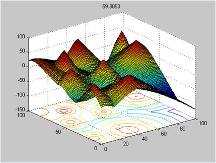
Also, each firefly i can move toward another more attractive (brighter) firefly j by equation
(2.2).
                                                                   1
                          xi = xi + β0 e−γrij (Xj − Xi ) + α(Rand − )
                                           2
                                                                                              (2.2)
                                                                   2

  Where α is a significance factor of randomization parameter and Rand with uniform distribu-
tion U(0,1) is a random number obtained from uniform distribution.

  Recently, some studies reveal efficiency of this algorithm(Yang, 2009) by outperforming other
meta-heuristic algorithms including some variation of particle swarm optimization(Łukasik and
Żak, 2009) and also, in dealing with stochastic test functions and noisy environments(Aungkulanon,
Chai-ead and Luangpaiboon, 2011). A more comprehensive description of this algorithm is
given in (Yang, 2008) . Also, a pseudo code of firefly algorithm is presented in Algorithm 1.

3 Proposed Algorithm

  In this section, a novel speciation based on firefly algorithm named SFA is presented for op-
timization in a dynamic environment. In the proposed algorithm, some modifications are done
on firefly algorithm for better performance in dynamic environment. First, the best personal
location of each firefly (Pbest) is added to the algorithm by inspiration from particle swarm opti-
mization. The best personal location of each firefly can only help algorithm to move toward the
best position. By holding Pbest of each firefly before fitness evaluation, algorithm can move to
a better position if fitness value decreases. Second, randomization parameter of the firefly (α)
is changed in an adaptive manner. The value of α increases if new location of firefly has better
fitness value than previous fitness value of the best personal location of that firefly, otherwise
it decreases.

  Also, in the proposed algorithm, there is only one swarm of fireflies which acts on the envi-
ronment. This is one of the most important differences between our proposed algorithm and
many other multi-population approaches. When the algorithm starts working, fireflies scatter
around the environment randomly. After a while of executing the firefly algorithm, speciation of
fireflies happens and fireflies swarm is divided into some species which each species moves
toward one local optimum. This is due to potential capability of firefly algorithm in converging
toward more than one local optimum if parameters have been set properly. But because many
local optima may exist in the environment, convergence to all of them requires a large popu-
lation of fireflies and a chance for good initialization. To solve this issue, an exploring swarm
is added which is responsible to explore the entire environment to find better solutions. If ex-
ploring swarm can find any better solution, the best point of exploring swarm will be added to
population. Therefore, firefly algorithm can converge to some local optimum which population
hasnt found them yet.

  Furthermore, to improve local search ability of the algorithm, the idea of quantum particles
has been used (Blackwell and Branke, 2006). Quantum particles used in this paper are com-
pletely different from prior application. They are used only to improve the convergence of global
best firefly in the population.
The pseudo code of proposed algorithm is presented in Algorithm 2 and applied routines are
shown in Algorithm. 3 to 6.
Algorithm 2: Proposed Algorithm (SFA)
1 begin
2 Initialize Parameters
3 Initialize fireflies swarm and discoverer swarm Randomly
4 while stop criteria is not satisfied do
5 call T est f or change()
6 Initialize test point
7 if Discovery is true then
8 Call Discovery()
9 end
10 if mod(iteration, discovery period) == 0 then
11 if number of fireflies in swarm is less than max f iref ly in swarm then
12 Add best discoverer to firefly swarm
13 else
14 Replace best discoverer with a firefly in swarm which has most fitness value
and at least a neighbor firefly is in radios of rneighborhood
15 end
16 end
17 call M ove f iref ly()
18 call U pdate best swarm()
19 end
20 end
In proposed algorithm, discovery period indicates how much iteration must be run until the
discoverer point is ready for adding to population. rneighborhood is neighborhood radios for each
firefly. If two fireflies has Euclidian distance less than rneighborhood , we say these fireflies
are very close to each other. When we want to add a new discoverer point to the swarm,
we try to add a point, which is not a neighborhood for other fireflies. M ax f irelf ly in swarm
indicate maximum number of fireflies which can be contributed in optimization process. Also,
we suppose best firefly as a test point for determining change in the environment.Algorithm 3: T est f or change()
1 begin
2 Evaluate test point
3 if new value of test point is different from previous fitness value then
4 Reinitialize rcloud and α
5 re-evaluate all fireflies in swarm
6 end
7 end
Algorithm 3 shows pseudo code of test f or change() routine. In this routine, rcloud is the
radios of quantum. With respect to (Blackwell and Branke, 2006) and (Blackwell et al., 2008) ,
quantum cloud value has to be determined based on peaks shift length.
Algorithm 4: Discovery()
1 begin
2 t=0
3 while t is less than discovery iteration do
4 Set a new point based on best firefly in discovery swarm by adding a random
vector number between -rcloud and rcloud to best firefly in discovery swarm
5 Evaluate new test point
6 if fitness of new point is better than best firefly in discovery swarm then
7 Set best firefly to this new point
8 Set rcloud by equation (3.1)
9 end
10 t=t+1
11 end
12 end
rcloud (t) = rcloud (t − 1) × (LLow + (Rand × (LHigh − LLow ))) (3.1)
Also, Algorithm 4 shows pseudo code of Discovery() routine. In equation (3.1), rcloud in each
iteration is obtained randomly based on its value at previous iteration. LLow and LHigh are lower
limit and upper limit of rcloud change percentage in compare with previous iteration. Rand is
the random number generator function with uniform distribution in [0, 1]. Hence, rcloud value in
each iteration randomly is in [rcloud (t − 1) × LLow , rcloud (t-1) × LHigh ]. For this reason, LHigh
value should be considered less than one and LLow ≤ LHigh . It should be mentioned that rcloud
value is initialized after every environment change to adapt itself with problem space conditions.Algorithm 5: M ove f iref ly()
1 begin
2 for i = 1 : n all n fireflies do
3 for j = 1 : n all n fireflies do
4 if Ii > Ij then
5 Move firefly i towards j based equation (2.2)
6 Evaluate new solution
7 if new fitness value is better than personal best fitness value then
8 Set personal best position to new firefly position
9 else
10 Set firefly position to previous personal best position
11 end
12 end
13 Attractiveness varies with distance r via exp[−γr2 ]
14 end
15 end
16 end
Algorithm 5 shows Pseudo Code of M ove f iref ly() routine. It shows some difference with
standard firefly algorithm which described yet.
Algorithm 6: U pdate best swarm()
1 begin
2 for counter =1 to try number do
3 Update Quantum based on equation (3.2)
4 if f(Quantum) > f(Global best) then
5 Global best = Quantum
6 end
7 end
8 update rcloud based on equation (3.1)
9 end
xQuantum,j = Global best + (rcloud × Rj ) (3.2)
Algorithm 6 show pseudo code of update best swarm() routine. In equation (3.2), Rj is a
random number with uniform distribution in [-1, 1]. So component jth of quantum firefly locates
at [−rcloud ,rcloud ] around the same component in global best of the firefly swarm. Therefore,
quantum firefly position would place in a d-dimensional ball around global best of the firefly
swarm. Also, try number specify number of try to improve global best firefly of swarm.4 Experimental Study
To evaluate correctness and efficiency of the proposed algorithm, this algorithm was com-
pared with some well-known algorithms on Moving Peaks benchmark (MPB) which is one of
the most famous benchmarks for dynamic environments. In this section, first MPB introduced
and then needed experimental setting is given. After that, we study effect of shift severity,
number of peaks and environmental change frequency on proposed algorithm.
4.1 Moving Peaks Benchmark (MPB) problem
Moving Peaks Benchmark(Branke, 1999) is widely used for evaluating the performance of
opimization algorithms in dynamic environments. In this benchmark, there are some peaks in a
multi-dimensional space, where height, width and position of peaks alter when a change occur
in the environment. For the D-dimensional landscape, the problem is defined as equation (4.1):
F (→
−
x , t) = max(B(−
→
x ), maxP (−
→
x , hi (t), wi (t), −
→
p i (t))) (4.1)
Where hi (t) and wi (t) are the height and width of peak i at time t, respectively, and pi (t) is
the position of peak i at time t. The p independently specified peaks are blended together by
the max function. The position of each peak is shifted in a random direction by a vector −→v i
of a distance s (s is also called the shift length, which determines the severity of the problem
dynamics), and the move of a single peak can be described as equation (4.2):
→
−
vi (t) = −
S
((1 − λ)−
→
r + λ−
→
vi (t − 1)) (4.2)
|→
r +−
→
vi (t − 1)|
Figure 1: Shape of Moving Peaks Benchmark Problem.
Where the shift vector − →vi (t) is a linear combination of a random vector −
→r and the previous
−
→
shift vector vi (t − 1) and is normalized to the shift length s. the correlated parameter λ is set
to 0, which implies that the peak movements are uncorrelated. More formally, a change of asingle peak can be described as equation (4.3):
σ ∈ N (0, 1)
hi (t) = hi (t − 1) + heightseverity ∗ σ
(4.3)
wi (t) = wi (t − 1) + widthseverity ∗ σ
−
→
p (t) = −→
p (t − 1) + →−
v (t)
i i i
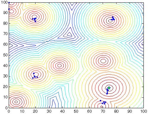
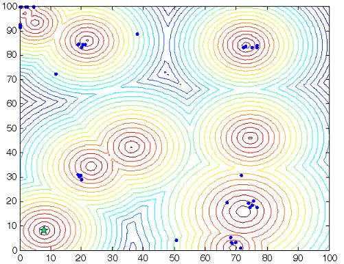
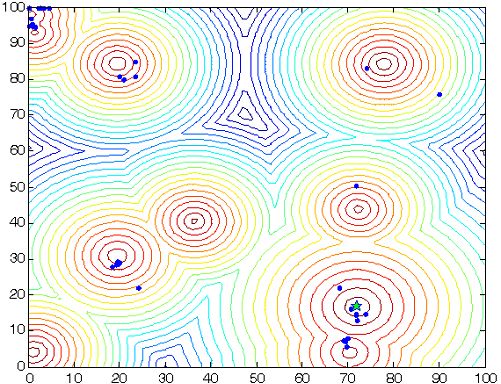
Also, for the shape of function P , Cone and Hilly shape function can be selected. Shape of
MPB and movement of the peaks in the landscape for four changes in environment showed in
figure. 1 and 2.
a)F irst change b)Second change
c)T hird change d)F ourth change
Figure 2: Movement of the peaks in the landscape for four changes in the environment.
Experiments were done with respect to MPB parameters setting which are given in table (1).Table 1: MPB parameters setting.
Parameter Value
Number of peaks, M Variable between 1 to 200
Change frequency 5000
Height change 7.0
Width change 1.0
Peaks shape Cone
Basic function No
Shift length, s 1.0
Number of dimensions,D 5
Correlation Coefficinet, 0
peaks location range [0 100]
Peak height [30.0 70.0]
Peak width [1 12]
Initial value of peaks 50.0
4.2 Experimental setting
Adjustment of parameters values in the proposed algorithm are as follows:
At the beginning of execution, algorithm starts with 5 fireflies in population, and maximum num-
ber of fireflies which can contribute in execution limited to 100 fireflies. It was proved (Blackwell
et al., 2008) that this number of particles has the best efficiency in solving MPB problem. It was
shown (Blackwell et al., 2008) that adjusting rcloud value equal to half of shift length would give
proper results, so we consider this as initialized value of rcloud too. According to various exper-
iments have been done it concluded that adjusting try number equal to 50 and also LLow and
Lhigh equal to 0.6 and 1 would give appropriate results. The primary performance measure is
the offline error (Branke and Schmeck, 2003) which is the average over, at every point in time,
the error of the best solution found since the last change of the environment. This measure is
always greater or equal to zero and would be zero for perfect tracking. Experiments were re-
peated independently 50 times and each time they were performed by different random seeds.
Every experiment continued until environment changes 100 times. For example when change
frequency was 5000, experiments performed 5 × 10⁵ fitness evaluations and during this time
the environment changes 100 times.
4.3 Experimental investigation of SFA
In this section, we study effect of varying shift severity, number of peaks on proposed algorithm.
4.3.1 Effect of varying shift severity
In this section, the performance of proposed algorithm is compared with six other algorithms
which are mQSO (Blackwell and Branke, 2006), AmQSO (Blackwell et al., 2008), mCPSO(Blackwell and Branke, 2006), SPSO (Du and Li, 2008), rSPSO (Bird and Li, n.d.) and PSO-
CP (Liu et al., 2010) on the MPB problems with 10 peaks, change frequency 5000 and different
settings of the shift length (vlenght). The experimental results regarding the offline error and
standard error are shown in Table 2.
Table 2: Effect of varying shift severity.
Shift Severity
Algorithm 1.0 2.0 3.0 5.0
mQSO 1.75(0.06) 2.40(0.06) 3.00(0.06) 4.24(0.10)
AmQSO 1.51(0.10) 2.09(0.08) 2.72(0.09) 3.71(0.11)
mCPSO 2.05(0.07) 2.80(0.07) 3.57(0.08) 4.89(0.11)
SPSO 2.51(0.09) 3.78(0.09) 4.96(0.12) 6.76(0.15)
rSPSO 1.50(0.08) 1.87(0.05) 2.40(0.04) 3.25(0.09)
PSO-CP 1.31(0.06) 1.98(0.06) 2.21(0.06) 3.20(0.13)
SFA 1.05(0.08) 1.44(0.06) 2.06(0.07) 2.89(0.13)
4.3.2 Effect of varying number of peaks
In table 3, efficiency of proposed algorithm are compared with ten other algorithms include
mQSO, mCPSO, AmQSO, CellularPSO(Hashemi and Meybodi, 2009), FMSO(Li and Yang,
2008), RPSO(Hu and Eberhart, 2002), SPSO, rSPSO, mPSO(Kamosi, Hashemi and Meybodi,
2010) and PSO-CP on the MPB problems with various number of peaks, change frequency
5000 and shift length 1. The results of some algorithms obtained from their papers. As can be
seen in this table, the proposed algorithm has much better performance than other algorithms.
In fact, the results show the proposed algorithm is robust with number of peaks and when the
number of peaks is low or when the number of peaks is high can achieve acceptable results.
Table 3: comparison of offline error (standard error) of 11 algorithms on MPB problem with
different number of peaks
Number Of Peaks
Algorithm 1 5 10 20 30 50 100 200
mQSO 4.92(0.21) 1.82(0.08) 1.85(0.08) 2.48(0.09) 2.51(0.10) 2.53(0.08) 2.35(0.06) 2.24(0.05)
AmQSO 0.51(0.04) 1.01(0.09) 1.51(0.10) 2.00(0.15) 2.19(0.17) 2.43(0.13) 2.68(0.12) 2.62(0.10)
CLPSO 2.55(0.12) 1.68(0.11) 1.78(0.05) 2.61(0.07) 2.93(0.08) 3.26(0.08) 3.41(0.07) 3.40(0.06)
FMSO 3.44(0.11) 2.94(0.07) 3.11(0.06) 3.36(0.06) 3.28(0.05) 3.22(0.05) 3.06(0.04) 2.84(0.03)
RPSO 0.56(0.04) 12.22(0.76) 12.98(0.48) 12.79(0.54) 12.35(0.62) 11.34(0.29) 9.73(0.28) 8.90(0.19)
mCPSO 4.93(0.17) 2.07(0.08) 2.08(0.07) 2.64(0.07) 2.63(0.08) 2.65(0.06) 2.49(0.04) 2.44(0.04)
SPSO 2.64(0.10) 2.15(0.07) 2.51(0.09) 3.21(0.07) 3.64(0.07) 3.86(0.08) 4.01(0.07) 3.82(0.05)
rSPSO 1.42(0.06) 1.04(0.03) 1.50(0.08) 2.20(0.07) 2.62(0.07) 2.72(0.08) 2.93(0.06) 2.79(0.05)
mPSO 0.90(0.05) 1.21(0.12) 1.61(0.12) 2.05(0.08) 2.18(0.06) 2.34(0.06) 2.32(0.04) 2.34(0.03)
PSO-CP 3.41(0.06) - 1.31(0.06) - 2.02(0.07) - 2.14(0.08) 2.04(0.07)
SFA 0.42(0.07) 0.89(0.09) 1.05(0.04) 1.48(0.05) 1.56(0.06) 1.87(0.05) 2.01(0.04) 1.99(0.06)5 Conclusion
In this paper, a new method for optimization in dynamic environments was proposed based
on speciation based firefly algorithm. Results on various configuration of moving peak bench-
mark problem were compared with several well-known methods. The proposed algorithm used
new mechanisms to divide population into some swarms. Totally, in this algorithm, it attempted
to satisfy all dynamic environments requirements. Experimental results showed that the pro-
posed algorithm has an acceptable performance than other algorithms.
Also, there are some relevant works to pursue in the future. First, some work can be done
to set a good initialization before the algorithm start. Second, some adaptation can be done
on fireflies parameters such as β and γ to improve efficiency of the algorithm. Third, some
works can be done to improve local search ability of algorithm by using prior knowledge of the
problem space.
References
Aungkulanon, P., Chai-ead, N. and Luangpaiboon, P. 2011. Simulated manufacturing process
improvement via particle swarm optimisation and firefly algorithms, Proceedings of the
International MultiConference of Engineers and Computer Scientists 2.
Bird, S. and Li, X. n.d.. Using regression to improve local convergence, Evolutionary Compu-
tation, 2007. CEC 2007. IEEE Congress on, IEEE, pp. 592–599.
Blackwell, T. 2003. Swarms in dynamic environments, Genetic and Evolutionary Computa-
tionGecco 2003, Springer, pp. 200–200.
Blackwell, T. 2007. Particle swarm optimization in dynamic environments, Evolutionary Com-
putation in Dynamic and Uncertain Environments pp. 29–49.
Blackwell, T. and Branke, J. 2004. Multi-swarm optimization in dynamic environments, Appli-
cations of Evolutionary Computing pp. 489–500.
Blackwell, T. and Branke, J. 2006. Multiswarms, exclusion, and anti-convergence in dynamic
environments, Evolutionary Computation, IEEE Transactions on 10(4): 459–472.
Blackwell, T., Branke, J. and Li, X. 2008. Particle swarms for dynamic optimization problems,
Swarm Intelligence pp. 193–217.
Branke, J. 1999. Memory enhanced evolutionary algorithms for changing optimization prob-
lems, Evolutionary Computation, 1999. CEC 99. Proceedings of the 1999 Congress on,
Vol. 3, IEEE.
Branke, J. and Schmeck, H. 2003. Designing evolutionary algorithms for dynamic optimization
problems, Advances in evolutionary computing: theory and applications pp. 239–262.Du, W. and Li, B. 2008. Multi-strategy ensemble particle swarm optimization for dynamic
optimization, Information sciences 178(15): 3096–3109.
Hashemi, A. and Meybodi, M. 2009. Cellular pso: A pso for dynamic environments, Advances
in Computation and Intelligence pp. 422–433.
Hu, X. and Eberhart, R. 2002. Adaptive particle swarm optimization: detection and response
to dynamic systems, Evolutionary Computation, 2002. CEC’02. Proceedings of the 2002
Congress on, Vol. 2, IEEE, pp. 1666–1670.
Janson, S. and Middendorf, M. 2004. A hierarchical particle swarm optimizer for dynamic
optimization problems, Applications of evolutionary computing pp. 513–524.
Kamosi, M., Hashemi, A. and Meybodi, M. 2010. A new particle swarm optimization algorithm
for dynamic environments, Swarm, Evolutionary, and Memetic Computing pp. 129–138.
Kennedy, J. and Mendes, R. 2002. Population structure and particle swarm performance,
Evolutionary Computation, 2002. CEC’02. Proceedings of the 2002 Congress on, Vol. 2,
IEEE, pp. 1671–1676.
Li, C. and Yang, S. 2008. Fast multi-swarm optimization for dynamic optimization problems,
Fourth International Conference on Natural Computation, IEEE, pp. 624–628.
Li, C. and Yang, S. 2009. A clustering particle swarm optimizer for dynamic optimization,
Evolutionary Computation, 2009. CEC’09. IEEE Congress on, IEEE, pp. 439–446.
Li, X., Branke, J. and Blackwell, T. 2006. Particle swarm with speciation and adaptation in a
dynamic environment, Proceedings of the 8th annual conference on Genetic and evolu-
tionary computation, ACM, pp. 51–58.
Liu, L., Yang, S. and Wang, D. 2010. Particle swarm optimization with composite particles
in dynamic environments, Systems, Man, and Cybernetics, Part B: Cybernetics, IEEE
Transactions on 40(6): 1634–1648.
Łukasik, S. and Żak, S. 2009. Firefly algorithm for continuous constrained optimization tasks,
Computational Collective Intelligence. Semantic Web, Social Networks and Multiagent
Systems pp. 97–106.
Lung, R. and Dumitrescu, D. 2007. A collaborative model for tracking optima in dynamic
environments, Evolutionary Computation, 2007. CEC 2007. IEEE Congress on, IEEE,
pp. 564–567.
Parrott, D. and Li, X. 2004. A particle swarm model for tracking multiple peaks in a dynamic
environment using speciation, Evolutionary Computation, 2004. CEC2004. Congress on,
Vol. 1, IEEE, pp. 98–103.
Parrott, D. and Li, X. 2006. Locating and tracking multiple dynamic optima by a particle swarm
model using speciation, Evolutionary Computation, IEEE Transactions on 10(4): 440–458.Petrowski, A. 1996. A clearing procedure as a niching method for genetic algorithms, Evo-
lutionary Computation, 1996., Proceedings of IEEE International Conference on, IEEE,
pp. 798–803.
Yang, X. 2008. Nature-inspired metaheuristic algorithms, Luniver Press.
Yang, X. 2009. Firefly algorithms for multimodal optimization, Stochastic Algorithms: Founda-
tions and Applications pp. 169–178.You can also read