High accuracy speed measurement using GPS (Global Positioning System)
←
→
Page content transcription
If your browser does not render page correctly, please read the page content below
High accuracy speed measurement using GPS (Global Positioning System)
                                         by Tom J. Chalko, MSc, PhD*
       ©Tom Chalko 2007, all rights reserved. This document may be distributed freely, providing that no content is modified

Abstract.
This article demonstrates that speed                                       Modern GPS devices implement digital PLL
measurement with accuracy approaching 0.01                                 (phase-lock loop) receivers to continuously
knot is possible by using GPS Doppler data.                                track carrier frequencies of a number of
The method is illustrated with measurements                                satellites. For example, GT-11 tracks carrier
made by GT-11 GPS unit made by Locosys.                                    frequencies of up to 12 satellites
                                                                           simultaneously. The frequency tracking has to
Introduction                                                               be continuous simply because each receiver
Typical approach to using GPS for speed                                    has to be always ready to receive data from its
measurement today is to consider a series of                               satellite.
“trackpoints” that record position estimates
(latitude and longitude) determined by the                                 The very fact that data is read from any given
GPS at regular time intervals.                                             satellite is proof that its carrier frequency is
                                                                           tracked with high accuracy.
Each GPS trackpoint is determined with some
error that is variable and difficult to                                    The difference between the known satellite
determine. Hence, speed values computed                                    carrier frequency and the frequency
from a series of trackpoints have unknown                                  determined at the receiver is known as a
accuracy and cannot be considered reliable. It                             “Doppler shift”. This Doppler shift is directly
is virtually impossible to prove the accuracy                              proportional to velocity of the receiver along
of speed computed from a recorded series of                                the direction to the satellite, regardless of the
trackpoints.                                                               distance to this satellite.

The most inaccurate is the method that tries to                            With multiple satellites tracked it is possible
estimate an average speed over some                                        to determine the 3D velocity vector of the
“accumulated distance” between trackpoints.                                receiver. In general, the more satellites are
Due to trackpoint inaccuracies, the line                                   tracked – the better the speed estimate.
connecting all track points is a zig-zag, even
if the real path of a speed competitor is a                                Accuracy of the Doppler tracking
smooth or straight line. Since the length of                               The Doppler speed measurement accuracy is
this zig-zag is always longer than a                                       not constant. It depends on the number of
smooth/straight line, the “average speed”                                  tracked satellites as well as on their
determined with the “accumulated distance”                                 geometrical distribution above the horizon.
method always overestimates the real speed.
The less accurate are trackpoints (the less                                For this reason it is important to measure this
accurate is a GPS unit) – the larger the                                   accuracy directly - together with the actual
estimated “average” speed and the more                                     speed determined from the Doppler shift if
impressive is the “achievement”…                                           possible.

Doppler                                                                    The most convenient way of verifying the
An alternative to measuring speed from series                              Doppler speed measurement accuracy is
of trackpoints is using the Doppler effect.                                recording the Doppler speed data of a
                                                                           stationary GPS receiver at regular time
                                                                           intervals. This method accounts for all
* Senior Scientist, Scientific Engineering Research
                                                                           known6 GPS-Doppler speed measurement
.

P/L, Mt Best, Vic 3960, Australia. All correspondence
should be sent to tjc@sci-e-research.com. Updated                          errors. Results of @1 hour recording using
article is at nujournal.net/HighAccuracySpeed.pdf                          GT-11 are presented in Fig.1.
2
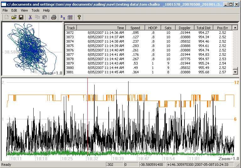
Fig.1. Comparison of Doppler speed and trackpoint-derived speed for stationary GT-11 using RealSpeed
software. Binary GT-11 data was logged for about 1 hour every second. Top-left: latitude-longitude
trackpoint trajectory. Top-right: a fragment of the data file (distance in meters, speed in knots). Bottom:
speed in knots: black – speed determined from trackpoints, green: Doppler speed, orange: number of tracked
satellites. Horizontal axis shows time in hours:minutes. The measured average Doppler speed is 0.0554 knot.
The position-derived average speed is 0.479 knots. The GPS unit was stationary, but the accumulated distance
computed from positions (trackpoints) is almost 1 km. Note the difference between HDOP (Horizontal
Dilution of Precision) and the gps-chip computed Position Error for each trackpoint.
10
1400 sa 0.14
mpl
1200 e
ave 0.12
rag
1000 e
Fre ma 0.1
gni
qu 800 tud
0.08
en e
cy 600 0.06
400 0.04
200 0.02
0 0
0 0.05 0.1 0.15 0.2
a)
0 1000 2000 3000
Magnitude [knots], µM =0.0554 ,σM =0.0287 b) time [s]
Fig.2. a) Measured distribution of the magnitude of Doppler measurement error in 1-second samples during 1-
hour observation. Discrete resolution is clearly visible with 1-bit corresponding to about 0.0194 knot (0.01
m/s). b) Doppler measurement error as a function of time. 10-sample average error magnitude is shown. 1-bit
resolution is constant (a), but the Doppler measurement accuracy varies in time.
Doppler accuracy at non-zero speed We need to remember that Earth spins. A
What will happen to the Doppler speed point that seems stationary with respect to the
resolution and accuracy for non-stationary surface of the Earth actually moves West-to-
GPS? East with speed in the order of 700 knots in
the geocentric frame of reference. (698 knots3
at Sandy Point, Vic, Australia). Yes, every v k = v kD − v ke . For a discrete series of speed
parked car can receive a speeding fine !!! samples vkD acquired at N uniform time
intervals over the time T we can approximate
Hence, from the point of view of the PLL the integral in the equation (2) by a sum and
Doppler frequency tracking system the expression for the unknown average speed
implemented in GPS devices it actually does becomes
not matter whether we try to measure speed of
∑ ∑
N N
700 knots, 650 knots or 750 knots. v v
v= k =1 kD
− k =1 ke
(4)
= v D − ve
) ) )
N N
Improving the accuracy by averaging The first term v D is the exact average of all
)
In their wisdom, developers of GT-11 enabled measured Doppler samples; the second term
continuous logging of low-pass filtered ve represents the measurement error. Other
)
Doppler speed data at 1 second intervals. This
methods of integration of the discrete series
enables us to evaluate the average speed with
are discussed later in this article.
greater accuracy than the accuracy of a single
Doppler sample.
Measurement errors vke of each sample can be
considered a series of independent random
Let’s begin with recalling the universally
variables that share the same probability
accepted definitions of speed and the average
distribution D. Fig 2 demonstrates that both
speed. Consider object moving along path P
the expected value µ and the standard
and traveling the distance ∆l during the time
deviation σ of D exist and are finite. A typical
interval ∆t = t2 – t1.
measured distribution of the magnitude of the
t1 t2 speed error vke is shown in Fig 2. In reality,
the probabilities of errors vke increasing and
P ∆l decreasing the measured values of speed are
equal. Hence each random variable vke can be
The speed v of the object is defined as
considered to have µ =0 and σ < σM + µM,
∆l dl where µM is he expected value and σM is the
v = lim ∆t →0 = (1)
∆t dt standard deviation of the measured magnitude
The average speed v̂ over time T is defined as of the speed error vke.
a time average of v as follows:
∫ ∫
T L
vdt dl The standard error σ v) of the measured average
L
vˆ = (2)
t =0 0
T T
= =
T speed v̂ can be determined directly from the
Definition of the average speed determines Central Limit Theorem5 to be:
unique relationship between the travelled σ v) = σ v)e =
σ
< M
µ +σ M
(5)
distance L (measured along the path P) and N N
the average speed v This error is inversely proportional to N
)
L = vT (3) and hence it decreases with the number of
)
It is important to point out that the average sampling intervals. As the number of
speed over the time T and the average speed sampling intervals N increases, the
over the distance L are identical: there exists distribution of σ v) approaches the normal
only one average speed that describes motion. distribution, enabling us to determine the
For this reason, the average speed is the best claimed average speed v with any required
)
possible measure of speed in sports that use
confidence level.
speed for their ranking.
In the absence of measured µM and σM the
In real measurements, each discrete GPS-
standard error σ specified by the GPS
Doppler speed sample vkD contains
manufacturer for Doppler speed should be
measurement error vke. Hence true speed vk is
used.4
N 1 ∆t1 + N 2 ∆t 2
2 2
σ v) = σ v)e = σ (7)
Non-uniform sampling intervals N 1 ∆t1 + N 2 ∆t 2
When multiple GT-11 units are used to This formula is easily extendable to
sample GPS-Doppler speed at 1Hz each, it is accomodate K diffferent sampling intervals as
possible to synchronize their sampling follows:
sequences to achieve GPS-Doppler speed
∑N
K
∆t k
2
samples at sub-second intervals, because all k
GT-11 units report their samples in UTC time σ v) = σ v)e = σ
k =1
. (8)
∑ N k ∆t k
K
with 1ms accuracy. Initially set time
“skewing” has been found maintained for k =1
many hours (providing that all synchronized For K=1 this formula gives equation (5) with
GT-11 units kept tracking satellites) and N being the number of sampling intervals ∆t
hence provides us with a method to increase during the time T.
the GPS-Doppler sampling frequency.
Rectangular rule of integration
Ideally, when K GT-11 units are used, each So far we approximated the intergral in the
second should be divided into K equal equation (2) by a simple sum of discrete
sampling intervals. However, in practice, K terms. This method of integration is referred
sub-second intervals may not be equal. For to as a “rectangular rule of integration”8. In
this reason we need to determine the average this rule it is assumed that the integrated
speed and its standard error for such a function does not change between samples.
situation. vD vD
Without loss of generality we may consider
the case of K=2 GT-11 units and the
t t
corresponding 2 sub-second time intervals ∆t1
and ∆t2, because as we shall soon see the K=2 Fig 3. Comparison of Left Riemann and Right
case is extendable to any K. The integral in Riemann approximation in the rectangular rule of
integration.
equation (2) can be approximated by a
For a large number of discrete samples Right
discrete sum of samples as follows
Riemann, Left Riemann approximations (as
∑ v ∆t1 + ∑ k =211 v kD ∆t 2
N1 N
k =1 kD well as midpoint approximation that is not a
v= + convenient option for samples of an unknown
)
N 1 ∆t1 + N 2 ∆t 2
(6) function) methods converge to the same
∑k =1 vke ∆t1 +∑k =21 vke ∆t 2
N1 N
result, but it is clear that for a limited number
− = v D − ve of experimentally acquired samples the
) )
N 1∆t1 + N 2 ∆t 2
rectangular rule of integration can be a source
where N1 and N2 are numbers of sampling
of ambiguity.
intervals ∆t1 and ∆t2 respectively in T and N =
N1 + N2. The first term represents v D (the
Trapezoidal Rule of integration
)
exact average of all measured Doppler vD
samples); the second term represents ve (the
)
measurement error). Applying the Central
Limit Theorem5 to each term in the numerator
of ve and implementing the theorem t
)
governing addition of variances of
independent variables8 we obtain the Fig 4. Trapezoidal rule of integration offers excellent
accuracy for a limited number of discrete samples and
following expression for the standard error eliminates the ambiguity associated with the
σ v) of the average speed v̂ : rectangular rule of integration5
Integration accuracy of an unknown function For K=1 this formula gives the equation (5)
represented by a limited number of discrete providing that Nk is the number of sampling
samples can be improved and ambiguity intervals ∆tk during the time T.
associated with the rectangular rule of
integration can be eliminated by Simpson Rule of integration
implementing the so-called “trapezoidal rule The so-called Simpson rule8 of integration of
of integration”8. discrete series of samples uses parabolas to
interpolate between discrete samples and is
It is important to point out that in the regarded as more accurate than the trapezoidal
rectangular method of integration the number rule. Although it is possible to use the
of GPS-Doppler samples N is equal to the Simpson rule to compute v D and estimate the
)
number of the sampling intervals during the
standard error σ v) of the corresponding
time T (see Fig 3) and all samples are given
the same weight. average speed, the gain in the accuracy is
likely to be too small to be worth an effort.
In contrast, the trapezoidal rule requires one
extra sample and requires the first and the Average of M speed attempts
last sample in the interval T to be given In some sports ranking is based on the
weight of 0.5. average speed of several attempts (runs). If
the number of attempts is M , the standard
For a uniform sampling period (K=1) the error of their average speed is:
trapezoidal rule can be expressed as follows:
∑σ
1 M
2
, (12)
∑
N σ v)e = k
v
v + v ND M k =1
vD = k =1 kD
− 0D (9)
where σ k is the standard error of the average
)
N 2N
where v0D and vND are the first and the last speed of the k-th attempt.
samples in the integration interval T. The
expression for v D in the general case of K Claimed speed
)
durations of sampling intervals is: In sports that base their rankings on the
∑ m =1 ∑ k =1 kD
K NK achieved average speed it is convenient to
v ∆t m v0 D ∆t1 + v ND ∆t K
vD =
)
− introduce the concept of “claimed average
∑ k k ∑ N k ∆t k speed”, being the average speed that can be
K K
N ∆ t 2
k =1 k =1 claimed to have been achieved with the
(10) required level of confidence in the presence of
measuring errors. Let’s define the claimed
where N = ∑ N k , and ∆t1 and ∆tK are the
K
speed as
(13)
k =1
vCLAIMED = v D − c σ v)
corresponding (the first and the last) sampling
) )
intervals. Fig 5 illustrates the fact that by adopting c=2
we can claim with 97.725% confidence that the
Using the same tools as in the previous claimed average speed has been achieved.
section of this article we can estimate the
standard error σ v) of the unknown average 2.275% 97.725%
speed v̂ obtained using the trapezoidal rule of
integration to be:
v CLAIMED Average
2σ v)
∑N
∆t ∆t
)
2 2
Speed
98
K
∆t k − 1 − K
2 )
2 2
k vD
) )
σ v) = σ
k =1
(11)
∑ N k ∆t k
K Fig. 5. Relationship between the measured average
speed v D and claimed speed for c =2
)
k =16
The graph in Fig 6. illustrates relationship Examples
between the coefficient c and the If a speed contest was made at the location
corresponding confidence level of the claimed and during the time I recorded the data
speed. presented in Fig 1. and Fig 2, an average of
10 consecutive 1-second Doppler readings
It is clear that if we ignore measurement could produce an average speed over 10
errors (c=0) we can claim with 50% seconds with accuracy of 0.044 knot and 95%
confidence that v D has been achieved.
) confidence (assuming σ =0.0841 knot). The
accuracy of the average speed of 5 * 10-
2.2 c second intervals would be 0.019 knots.
2
1.8 If four GT-11 units were used simultaneously
1.6
1.4 for a 20 second run (500m run at ~50 knots),
1.2 the speed measurement accuracy should be
1
0.8 about 0.015 knot with 95% confidence and
0.6 0.019 knot with 98% confidence.
0.4
0.2 Level of confidence in %
0 50 60 70 80 90
Proof of Speed
Fig 6. Relationship between the coefficient c and the Perhaps the most important feature of the
confidence level of the claimed speed in the range 50% GPS-based Doppler method for measuring
to 99% for normal distribution of σ v) speed is that it can actually provide a proof of
speed.
Increasing N
Regardless of the method of integration used, Using the Doppler data it is possible to prove
the accuracy of the average speed increases that certain average speed with respect to the
with the total number of samples and gound was maintained for a certain amount of
sampling intervals N in the interval T. N can time, because the Doppler method is trackable
be increased in three ways: increasing the back to Units of Measurement.
time T for measuring the speed and/or
increasing the sampling frequency and/or Proof of speed is possible even though we
increasing the number of GT-11 units that may not be able to prove an exact location
measure the same average speed. where that speed was achieved.
Increasing the number of GT-11 units to Incidentally, this is not the first time such a
measure the same average speed (using an problem occurred. It is well known in physics
array of GPS units) has rather profound that it is impossible to determine both velocity
consequences for the accuracy of speed and position of an electron. We can accurately
measurement using the GPS-Doppler method. determine one or the other, but not both…
Theoretically speaking, very high accuracy in Form my tests presented in Fig 1 it is obvious
the average speed measurement can be that GPS trackpoints should never be used to
achieved using the GPS-Doppler method, estimate the speed. Trackpoints can only
providing that sufficiently large GPS serve as a verification of the integrity of the
instrument array is used. Doppler speed data.
This is possible, because Setting up a Speed Contest
1. The measurement error decreases with Since the Doppler speed accuracy varies with
increased number of samples N the number of tracked satellites and their
2. GPS-Doppler speed samples acquired distribution above the horizon, there is a need
by individual GPS units are to determine and monitor this accuracy during
independent every serious speed event.7
The variability range of the standard speed Aliasing may occur if the bandwidth of the
error σ is not large, but observable. In two sampled Doppler process is too high in
days of experimenting near Sandy Point, comparison to the sampling frequency. The
Victoria, Australia I observed the average Nyquist criterion requires the sampling
Doppler standard speed error σ values ranging frequency to be at least twice the maximum
from 0.05 to 0.1 knots. Fig 1 (bottom) and Fig frequency present in the sampled process.
2b illustrate this variability.
When a sattelite phase is steady enough to
One way to determine the actual accuracy of admit this satellite data for position and speed
Doppler speed measurement during any given calculations, the bandwidth of a typical Phase
event is to use 2 identical GPS units like GT- Lock Loop filter that tracks this satellite
11 for the entire duration of the event, one signal is 2Hz.
unit placed in a stationary location and the
other placed on a moving craft or person. The This means that in order to eliminate aliasing
theoretical basis for this procedure is the fact errors the following solutions are available:
that reasons for Doppler signal errors6 are
common for multiple units that are 1. Use 4Hz GPS-Doppler sampling rate.
sufficiently close to one another and hence the This can be accomplished ether by using
corresponding speed error distrubutions are one GPS unit that is capable of reporting
correlated. Doppler samples at 4Hz or four 1Hz GPS
units synchronized to provide Doppler
Care should be taken that a similar number of samples approximately every 250ms.
satellites are visible from both units. In case 2. When sampling frequency is limited to F
of speed windsurfing for example this is (for example 2Hz for twin GT-11 units),
equivalent to the requirement of installing the mechanical motion of the GPS unit used
GPS unit on top of a helmet so that is never to measure speed should not contain
under water. frequencies above F/2 (1Hz in our
example). Mechanical vibrations of the
An alternative method would be to use one GPS unit with frequencies above F/2
GPS unit, but make it motionless for a few (above 1Hz in our example) should be
minutes before and after each speed attempt. filtered either using a seismic suspension
or biofeedback (locating the GPS on a
Doppler used in track data head of the competitor).
It is important to note, that 0.05 m/s (@0.1
knot) accuracy in speed over 1 second interval Implementation of the second solution is
is equivalent to 5 cm track position accuracy. described in the Reference 7.
GPS chipset developers know this very well Spoofing
and actually use Doppler speed measurement Opponents of direct measurements of
to improve the accuracy of trackpoints. average speed claim that it is possible to boost
the average speed result by inducing
Unfortunately, algorithms that mix Doppler transverse oscillations and thereby increasing
and satellite distance data are proprietary and the length L of the travelled trajectory. Let's
their unknown properties cannot be used to explore the upper limit of this boost in the
prove the speed or position. sport of speed windsurfing.
Consider transverse harmonic oscillations
Aliasing with peak-to-peak stroke S [m], and frequency
The accuracy analysis presented above in this f [Hz] superimposed on motion with velocity
article is valid only when GPS-Doppler speed V [knots]. When speed is sampled with
samples are free from aliasing errors. frequency F, the maximum frequency of
oscillations that can be recorded is f=F/2.8
If oscillations are optimally phase- actually reduce the average speed boost,
synchronized with the sampling process, because not all samples used in the average
samples will contain the maximum possible speed calculation will contain the full amount
average transverse velocity SF during the of the boosted speed.
stroke. The corresponding speed boost εB is: In view of the above analysis we have to
conclude that, providing that aliasing is
ε B= V 2 + (1.944 SF ) − V [knots],
2
eliminated, effects of transverse oscillations
where the factor 1.944 converts m/s to knots. can be considered insignificant for speeds
For sampling rate F=1 Hz and speed V=40 above 30 knots when speed recording GPS
knots this means that a machinery of 1m in units are installed on/inside helmets of
size that generates motion precisely phase windsurfing sailors.
synchronized with the GPS sampling process
is required to boost the average speed by just Future of GPS technology
0.05 knots. Such machinery is not only illegal Today GT-11 unit provides 0.01 m/s speed
in sailing, but will introduce extra drag and measurement resolution and 0.1 m/s accuracy
hence reduce the sailing speed. for each one-second sample.
For many reasons (such as satellite The short term future of hand-held GPS
visibility, signal strength, reliability and devices can be predicted by studying
accuracy of GPS measurements) it is specifications of newly released GPS
recommended that speed-recording GPS units microprocessor chipsets that haven’t yet
to be worn on/inside a helmet7 worn by a found their way to the mass market.
sailor. The stroke S of human head is limited
to about 0.1 m. The corresponding upper limit These specifications indicate that as soon as
of speed boost that can be achieved at V=40 2008 we can expect GPS devices offering
knots is 0.00047 knots. 0.01 m/s Doppler speed accuracy for each
0.04
sample. It is rather interesting that the
positional (trackpoint) acurracy will remain
0.03 around 2.5 meters.
This seems yet another significant argument
0.02
0.01 to commit to Doppler method for speed
measurement.
0 0.2 0.4 0.6 0.8 1
S [m]
Fig 7. Maximum possible speed boost [knots] as a Conclusions
function of stroke for 1Hz speed samples at V=40 - Doppler shift is directly proportional to
knots.
speed. Hence, measuring Doppler shift is
the most direct and hence the most
At World Record speed V=50 this upper limit
accurate way of measuring speed.
for the speed boost is 0.00038 knots.
- Doppler frequency is relatively insensitive
Let's now explore increasing the frequency to distances from satellites, phase delays
of oscillations f to increase the speed boost. and many other factors6 that are major
Human head cannot move with frequency sources of errors for trackpoints
faster than 2 Hz and stroke larger than about - Doppler method of speed measurement
5cm (0.05m). Due to the upper frequency provides proof of speed, because it is
limit, the maximum possible speed boost trackable to Units of Measurement
would be achieved when speed is sampled at - Tolerance and accuracy of Doppler
4 Hz. The corresponding "maximum measurement can easily be measured and
physiologically achievable speed boost" at monitored experimentally
V=50 knots would be 0.0015 knots. Speed
sampling at rates higher than 4 Hz will9
- Accuracy of Doppler speed measurements 5. Wikipedia: Central Limit Theorem
can be significantly improved by adopting en.wikipedia.org/wiki/Central_limit_theor
the average speed as a measure of speed em
- Accuracy of the average speed 6. Jason Zhang, Kefei Zhang, Ron Grenfell,
measurement over given amount of time On the relativistic Doppler Effects and
interval increases with the number of high accuracy velocity determination
Doppler speed samples in this interval. using GPS, Proceedings of The
- Very high accuracy in the average speed International Symposium on GNSS/GPS,
measurement can be achieved today Sydney, Australia, 6–8 December 2004,
providing that sufficiently large number of http://www.gmat.unsw.edu.au/gnss2004u
suitable GPS instruments (GT-11) is used nsw/ZHANG,%20Jason%20P66.pdf
to measure the speed 7. T. Chalko, 2Hz GPS speed sailing helmet,
- Doppler speed measurements are mtbest.net/speed_sailing_helmet.html
repeatable and reproducible with 8. E. Kreyszig, Advanced Engineering
experimentally verifiable accuracy and Mathematics, 8th edition, John
resolution Wiley&Sons 1999
- The most practical method of computing
the average speed from GPS-Doppler
samples is to use the trapezoidal rule of
integration.
GPS Doppler tracking data from multiple
satellites provides a very accurate and very
easy way of measuring average speeds. The
longer the measuring period is, the more
frequent are Doppler speed samples and the
more GPS units are used simultaneously to
measure the same speed - the better the
accuracy.
For a speed event of 20 seconds or more, the
average speed measurements with accuracy as
high as 0.01 knot is possible with technology
that exists today: the GT-11 unit from
Locosys.
Are we ready to know the Real Speed we
achieve?
Really?
References
1. Locosys GT-11 GPS unit User Manual
www.locosystech.com/product.php?zln=e
n&id=5
2. M. Wright, RealSpeed software,
intellimass.com/RealSpeed/Index.htm
3. SiRF Binary Protocol Reference Manual
www.sirf.com
4. Wikipedia: Margin of error.
en.wikipedia.org/wiki/Margin_of_errorYou can also read