State Capacity, Property Rights, and External Revenues: Haiti, 1932-1949
←
→
Page content transcription
If your browser does not render page correctly, please read the page content below
State Capacity, Property Rights, and External Revenues:

                                    Haiti, 1932-1949

                                         Craig Palsson
                               Huntsman School of Business
                                    Utah State University
                                   craig.palsson@usu.edu

                                          July 6, 2021

                                            Abstract

   Investments in fiscal capacity are blunted by access to external revenues. But how do external
revenues affect investments in legal capacity? According to a simple model of state capacity
investment, external revenues and investments in legal capacity should be positively correlated.
I test this prediction by looking at Haiti in 1942 when U.S. mobilization caused a negative
shock to external revenues. I show the fall in revenues led to the state increasing investments
in legal capacity and property rights security. I account for this inconsistency by showing that
institutions can alter how states invest in capacity.

                                                1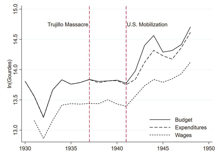
A growing consensus among economic historians and development economists is the role of state
capacity in economic development (Besley and Persson 2009, Johnson and Koyama 2017, Dincecco
2015). Given its importance, it is crucial to understand why developing countries do not invest in
state capacity. It is well established that countries invest less in fiscal capacity (the component of
state capacity that enables the government to collect internal tax revenues) when they have access to
external revenues through international trade (Frankema and Booth 2019, Gardner 2019). But we
do not understand how these external revenues affect investments in legal capacity, the component
of state capacity that enables the government to enforce property rights and the rule of law.
   To develop testable implications of the effect of external revenues on legal capacity, I use a simple
model of a state investing in capacity. The model has two periods where a state uses internal
and external tax revenues to provide public goods and, in the first period, invest in fiscal and
legal capacity. Consistent with the literature, the model shows that external revenues discourage
investments in fiscal capacity. In contrast, investments in legal capacity are increasing in external
revenues. The mechanisms for both are intuitive: internal taxes decrease private consumption, so
the state and citizens prefer external revenues over fiscal capacity; but investing external revenues
in legal capacity increases both private consumption and the public good, so there is a strong
incentive for investing in legal capacity. Yet, empirically, states where external revenues impeded
the development of fiscal capacity also tend to be states with low legal capacity. Thus, the model’s
predictions need to be examined empirically.
   To test the model’s implications, I turn to Haiti during the 1930s and 1940s. Through the
1930s, Haiti relied on customs revenues for over 80% of government revenues. But in 1942, the
Haitian government faced a sudden loss in customs revenues due to the United States’ entrance
into World War II. Consistent with the model, Haiti responded to the revenue shock by investing
in fiscal capacity. In 1942, Haiti reformed its income tax and increased tax rates on almost every
level of income. As a result, internal revenues doubled by 1944.
   To investigate the prediction that legal capacity is increasing in external revenues, I look at
Haiti’s public land rental program. The government leased public land to farmers and published
the property’s demarcation in its gazette, Le Moniteur. Using the universe of notifications published
from 1930 to 1949, I proxy for legal capacity using the average processing time between request
and approval. The average processing time for properties requested just before U.S. mobilization
was between 30 to 40 months. A major contributor to such long delays was a demand surge
caused by Haitian refugees from the Dominican Republic. To see how the external revenue shock

                                                  2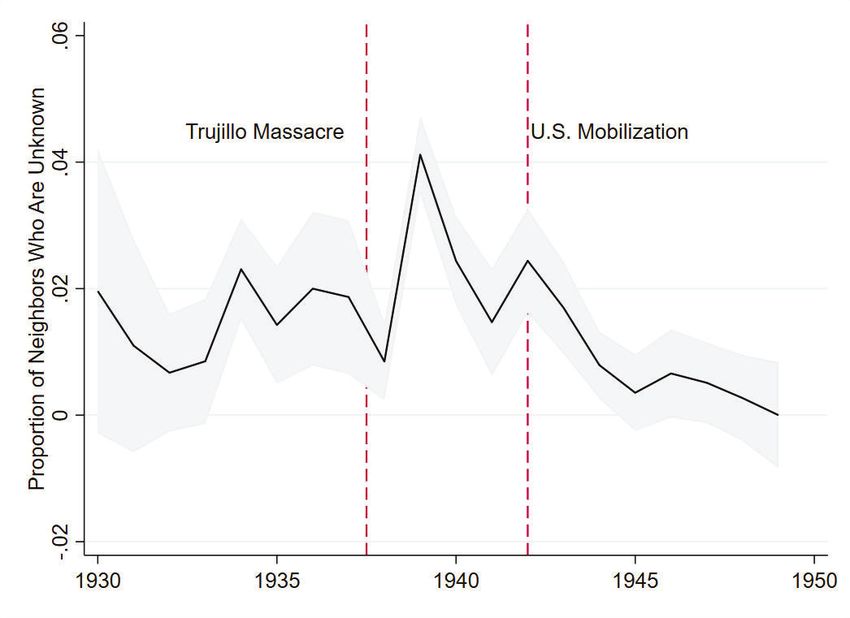
changed legal capacity (i.e. delays), I use a hazard analysis, which can account for changes in state
capacity that occur while properties are under review. The survival curves show that after U.S.
mobilization, the probability that approval would take longer than eight months dropped from 85%
to 20%. Moreover, the large reduction in delays occurred while request volume remained high.
Such a change suggests legal capacity increased. I confirm this result with other proxies of legal
capacity: after U.S. mobilization, properties were less likely to have incomplete demarcation, and
the program collected more rents.
   The increase in legal capacity after a fall in external revenues shows the model of investing in
state capacity is incomplete. There are two reasons, in this context, why this is the case. First,
the model assumes the revenues from internal taxes and external taxes are fungible. But Haitian
institutions did not treat the two the same. The appropriations law did not allocate any customs
revenues to investments in legal or fiscal capacity—all investments had to come from internal
revenues. Thus, when the drop in external revenues triggered an investment in fiscal capacity,
the subsequent increase in internal revenues created an opportunity to invest in legal capacity. A
second reason legal capacity increased with fiscal capacity was because the same administration
ran tax collections and the land rental program. Hiring more personnel for collecting taxes gave
the land rental program more officers to survey properties.
   This paper furthers the work on state capacity by exploring the relationship between fiscal and
legal capacity. It has been previously established that Latin American countries have lower fiscal
capacity because of their access to customs revenue (Centeno 1997). This paper suggests that
because institutional arrangements could link fiscal and legal capacity, the lack of fiscal capacity
could explain the lack of legal capacity. A similar result was found in preindustrial France, where
low legal capacity allowed some regions to prosecute women for witchcraft. But when France
consolidated its fiscal regime in the 17th century, it also invested in legal capacity, and witch trials
declined (Johnson and Koyama 2014).
   Another unique contribution from this paper is the growth of state capacity without a direct
military conflict. Many accounts of building state capacity show the power of conflict to motivate
investments (Besley and Persson 2010, Arias 2013, Gennaioli and Voth 2015). Indeed, one argument
is that state capacity does not cause economic development, but development leads to increases in
state capacity because richer states are more likely to be plundered (Geloso and Salter 2020). But
with Haiti, there was no direct or implicit threat that inspired a coalition to shift their preferences
towards building capacity. While a global military conflict caused the initial shock, the investments

                                                  3
in state capacity came from a drop in external revenues.

1    Model of External Revenue and Investments in State Capacity

Although there is little empirical understanding of how external revenues affect legal capacity, the
theoretical argument is easy to establish in a simple model. The model uses Besley and Persson
(2009) as a starting point. Since the Besley and Persson model includes several mechanisms that
are not relevant to this paper, I distill the model into its fundamental pieces then incorporate
external revenues. There are two main results. First, external revenues discourage investments
in fiscal capacity, a result that is accepted in the literature (Frankema and Booth 2019, Gardner
2019). Second, investments in legal capacity are increasing in external revenues.
    Before presenting the model, we need to define fiscal and legal capacity. In Besley and Persson
(2009), investing in state capacity involves building infrastructure and institutions. So legal capacity
“reflects legal infrastructure such as building court systems, employing judges, and registering
property,” and fiscal capacity is “the build-up of institutions such as an administration (like the
IRS in the United States) for the collection of income taxes, a system for the monitoring of tax
compliance, etc.” Johnson and Koyama (2017) give more general definitions. Legal capacity is the
state’s ability to “enforce its rules across the entirety of the territory it claims to rule,” and fiscal
capacity is the state’s ability to “garner enough tax revenues from the economy to implement its
policies.”
    I operationalize these definitions of state capacity as follows. The model has two periods (s ∈
{1, 2}), and in each period, the citizen receives an endowment (Ys ). But because property rights
are uncertain, the fraction of the endowment that the citizen keeps is determined by legal capacity
(πs ∈ [0, 1]) such that the citizen keeps only πs Ys . The citizen also faces an income tax which is
determined by fiscal capacity (τs ). Thus, the citizen’s disposable income is (1 − τs )πs Ys .
    In both periods, citizens get utility from private consumption (c) and a public good (G):

                                        us = α ln(Gs ) + ln(cs ).                                   (1)

Note that I assume a log-linear utility function. This is a departure from the Besley and Persson
model, where they assume a linear utility function. The problem with a linear utility function is
that private consumption and the public good become perfect substitutes and the marginal utility
of both is constant. Thus, if the marginal utility of the public good is higher than that of private

                                                   4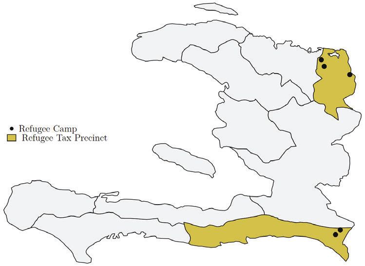
consumption, then the government wants to expand state capacity until it can tax 100% of income
and provide the public good. The conclusion is that states do not invest in capacity because the
citizens prefer private consumption. To allow for a trade-off between private consumption and the
public good, I assume a log-linear utility function.
   The government wants to maximize the citizen’s total utility across both periods. It gets revenue
from internal taxes (Ts = τs πs Ys ) and external (trade) taxes (Ms = M ≥ 0). In both periods, the
government uses revenue to supply a public good (Gs ). But in the first period, the government
can choose to invest in expanding state capacity for the second period, with the cost of investing
in legal capacity as L(π2 − π1 ) and the cost of investing in fiscal capacity as F (τ2 − τ1 ), with
F (0), L(0) = 0, F  (0), L (0) = 0, F  (x), L (x) ≥ 0 ∀x, and F  (x), L (x) ≥ 0 ∀x. Note that the
revenues for investing in capacity and providing the public good are fungible.
   Thus, the government’s objective function is


                                       max                         (α ln(Gs ) + ln(cs ))             (2)
                                G1 ,G2, c1 ,c2 ,π2 ,τ2
                                                         s∈{1,2}

subject to
                                                 cs = (1 − τs )πs Ys                                 (3)

                            G1 + L(π2 − π1 ) + F (τ2 − τ1 ) = τ1 π1 Y1 + M.                          (4)

                                                 G2 = τ2 π2 Y2 + M                                   (5)

   After using the constraints to solve for Gs and cs , there are two choice variables (π2 and τ2 ).
The first-order conditions are

                               αF  (τ2 − τ1 )                    απ2 Y2       1
                                                            =              −                         (6)
                  τ1 π1 Y1 + M − L(π2 − π1 ) − F (τ2 − τ1 )   τ2 π2 Y2 + M   1 − τ2

                                 αL (π2 − π1 )                     ατ2 Y2     1
                                                              =              +                       (7)
                    τ1 π1 Y1 + M − L(π2 − π1 ) − F (τ2 − τ1 )   τ2 π2 Y2 + M   π2

   Three important results emerge from the first-order conditions. First, there exists an M such
that the government chooses not to invest in fiscal capacity. To see this, suppose that the govern-

                                                              5
ment does not invest and τ2 = τ1 . Since F  (0) = 0, the M must satisfy the following identity:

                                           απ2 Y2       1
                                                    =        .                                      (8)
                                       τ1 π2 Y2 + M   1 − τ1

Thus,
                                   M = απ2 (1 − τ1 )Y2 − τ1 π2 Y2 .                                 (9)

Note that M could be equal to zero: even with no customs revenues, the government will not invest
in fiscal capacity because the marginal utility of extra fiscal capacity is not worth the cost of less
                                                                                                τ1
public good in the first period and less consumption in the second period. But M > 0 if α >     1−τ1 .

   The second result to note is that the government always wants to invest in legal capacity.
Suppose there was a condition where the government did not want to invest in legal capacity, such
that π2 = π1 . Then, from (7), the following identity must hold:

                                          ατ2 Y2     1
                                                   +    = 0.                                       (10)
                                      τ2 π2 Y2 + M   π2

But since both terms are positive (M cannot be less than zero), then this is a contradiction. Thus,
the government always wants to invest in legal capacity. Intuitively, this is because increasing
legal capacity carries two benefits: increasing both the public good and private consumption in the
second period.
   Third, although investments in fiscal capacity cease when M ≥ M , investments in legal capacity
continue and are increasing in M . Fiscal capacity brings the benefit of more public goods, but at
the costs of less private consumption. But M provides a source of revenue for investments that do
not decrease private consumption. So the government does not need more fiscal capacity. But it
wants to increase legal capacity because it is a way to transfer higher customs revenue to higher
private consumption.
   Thus, the model gives two testable predictions from a change in customs revenue. First, a
significant drop in customs revenue should cause the government to invest in fiscal capacity. Second,
the drop should cause the government to decrease investments in legal capacity. Yet, a casual
assessment suggests that the prediction for legal capacity might not hold. While countries with
high external revenues have low fiscal capacity, they often also have low legal capacity. If external
revenues do not increase legal capacity, the model assumptions needs to be reassessed. Thus, we
need an empirical investigation.

                                                  6
Table 1. Export Value and Taxex Collected by Haitian Government, 1932-1948

                        Export Value    External Revenues    Internal Revenues   Income Tax

      Pre-Reform
      1932                     36,106               23,036               3,931           438
      1933                     46,650               30,870               4,991           609
      1934                     51,546               30,283               5,049           527
      1935                     35,629               24,152               4,520           525
      1936                     47,239               28,799               4,695           465
      1937                     44,854               28,680               4,965           462
      1938                     34,732               22,515               4,991           476
      1939                     36,338               25,556               5,022           396
      1940                     26,995               21,153               5,246           469
      1941                     33,287               21,423               4,879           472

      Reform Partially Implemented
      1942                  42,886                  19,347               5,337           637

      Reform Fully Implemented
      1943                  53,073                  22,265              8,668         2,741
      1944                  80,542                  30,927             10,489         3,703
      1945                  85,562                  30,313             10,550         4,635
      1946                114,117                   32,519             10,878         4,364
      1947                157,492                   51,875             11,933         4,845
      1948                154,425                   57,328             18,105         9,449

Notes: Figures are in thousands of gourdes and not adjusted for inflation. The income tax is part
of internal revenues, and total tax revenues is the sum of external and internal revenues. Data
come from Annual Reports of the Fiscal Representative.

2    Haiti and the Fiscal Response to World War II

To test the model’s predictions, I use an external revenue shock caused by U.S. mobilization in
World War II. As the model predicts, this shock caused the government of Haiti to invest in fiscal
capacity.
    In the early 20th century, the Haitian government had little opportunity to collect internal
revenues because of the country’s poverty, but it also had little need for fiscal capacity because
of high customs revenues. In a 1927 report, officials supervising the American occupation said a
study of 34 countries found Haiti to be the most dependent on customs revenues (Haiti Bureau du
representant fiscal 1927 pp. 64-65). During the study period, trade taxes supplied about 90% of

                                                7
the government’s revenues, with internal revenues accounting for the other 10%. Its dependence far
exceeded the next two countries in the study: Salvador (66%) and the Dominican Republic (50%).
Table 1 shows that by 1941 Haiti’s dependence on external revenues had shrunk and supplied only
82% of government revenues. But the heavy dependence on customs became a critical weakness
when the U.S. entered World War II.
   At the close of 1941, when the U.S. mobilized in response to Pearl Harbor, the Haitian govern-
ment faced a budget crisis. America’s entrance into the war restructured Haiti’s trade, diverting
high-tariff imports like cars and cement. Customs receipts in 1941-42 were lower than at any point
in the previous 20 years, including every year of the Depression (Banque nationale de la Republique
d’Haiti 1942 p. 62). Anticipating the drop, the Haitian government rushed to find new revenues.
"Before many weeks of war had passed, it became evident that new methods would have to be de-
vised and special arrangements made in order to enable the country to ride out the storm" (Banque
nationale de la Republique d’Haiti 1942 p 2). The new sources included appealing to the U.S. for
help, receiving a line of credit from the Export-Import Bank, and passing a special tax on the
country’s largest export, coffee (Banque nationale de la Republique d’Haiti 1942 p. 2-3, 7). But
such measures were insufficient.
   Consistent with the model, the drop in customs stimulated investments in fiscal capacity. De-
spite the drop in trade taxes, the economy as a whole (using value of exports as a proxy) was
performing well, as seen in Table 1. Thus, a shrewd policy for a government desperate for rev-
enue was to increase internal revenues. In 1942, the government resorted to reforming the income
tax. Table 2 shows how the 1942 reform changed rates. The top tax rate in the old law was 6%,
but under the new law it soared to 15%. The old tax law treated business income (from societes
anonymes) differently than personal income. But the new law treated the two sources the same.
We do not know how much revenue the government collected from each bracket, but the median
rate increase was 70%. If the Haitian Internal Revenue Service (HIRS) could collect the revenues,
the reform should significantly increase internal revenues.
   The government had to overcome two barriers to collecting internal revenues. First, HIRS
needed more personnel. From 1926 to 1931, HIRS employed 80-90 rural agents responsible for
collecting communal taxes. By 1933, the number had jumped to 151, but the administrators had
little confidence in the new hires. “Due to the fact that there are many districts in which receipts
are so sparse that it is not possible to pay local agents adequate salaries for their collection, the
Internal Revenue Service is still considerably handicapped in getting honest and efficient local

                                                 8
Table 2. Haitian Income Tax Schedule, 1932 and 1942
Bracket 1932 Rate 1942 Rate Factor Increase
Personal Income
Less than 5,000 3% 3% 1.0
5,001–10,000 3% 4% 1.3
10,000–12,500 3% 5% 1.7
12,501–15,000 4% 5% 1.3
15,001–25,000 4% 8% 2.0
25,001–30,000 5% 8% 1.6
30,001–75,000 5% 12% 2.4
75,001–100,000 6% 12% 2.0
More than 100,000 6% 15% 2.5
Business Income
Less than 5,000 5% 3% 0.6
5,000–10,000 5% 4% 0.8
10,001–15,000 5% 5% 1.0
15,001–30,000 5% 8% 1.6
30,001–50,000 5% 12% 2.4
50,001–100,000 6% 12% 2.0
More than 100,000 6% 15% 2.5
Notes: Figures are in gourdes, unadjusted for inflation. Rates from 1932 come from Le Moniteur,
29 September 1932. Rates from 1942 come from Le Moniteur, 25 May 1942.
9officers. The turnover is consequently very large among these local agents,” (Haiti Bureau du
representant fiscal 1933 pp. 128-129). Moreover, only a fraction of the agents worked in the regions
outside of the western population center: the three regions bordering the Dominican Republic in
the East employed 36 agents total in 1933, and only 17 in 1931. After these years, we do not have
good data on how many tax collectors HIRS employed. But the data do show that expenditures on
personnel soared after the reform (see Figure 7 below). Specifically, in the first year of the reform,
“the staff of traveling inspectors was considerably increased” (Banque nationale de la Republique
d’Haiti 1943, p. 12). In a rural country with few major population centers, traveling inspectors
were crucial to collecting taxes.
The second barrier to improving revenue collection was the lack of physical capital to comple-
ment the personnel’s labor. To complement the newly hired traveling inspectors, HIRS purchased
new automobiles (Banque nationale de la Republique d’Haiti 1943, p. 12). Prior to the reform,
HIRS did not have much physical infrastructure. “The Internal Revenue Service maintains agen-
cies throughout the Republic, and many of these agencies in the past have been poorly housed
or completely lacking in Government owned quarters” (Banque nationale de la Republique d’Haiti
1944 p. 11). This changed with the reform. “A program of construction of internal revenue offices
was undertaken in the course of the year” (idem.). Furthermore, HIRS had historically struggled
to track who owed taxes, but with the new budget “the Internal Revenue Service also undertook
the construction of an archives building,” (Banque nationale de la Republique d’Haiti 1943, p. 12)
which was completed the next year (Banque nationale de la Republique d’Haiti 1944, p. 11).
These investments contributed to increasing tax revenues not just in the year the reform passed
but in the subsequent years as well. Table 1 shows that revenues before the reform averaged 484,000
gourdes per year. But in 1943, the first year the reform was fully implemented, the government
collected 2,741,000 gourdes, more than five times the pre-reform average. Then revenues increased
every year, reaching ten times the pre-reform average from 1945-1948, and even hitting 9,449,000
in 1949. The figures in Table 1 are nominal, but comparing them to total tax revenue shows the
increase was not a result of inflation. Before the reform, the income tax was about 10% of all
internal taxes. After the reform, the income tax became the most important source of internal
revenue, comprising 50% of total internal taxes by 1948. The substantial growth in income taxes
suggest the reform did more than just increase tax rates; it collected taxes more efficiently.
103 Legal Capacity in Haiti Before U.S. Mobilization
The remainder of the paper focuses on how the revenue shock from U.S. mobilization affected in-
vestments in legal capacity. I can observe legal capacity through a government land rental program.
3.1 Land Rentals and Legal Capacity
Like with all countries, measuring legal capacity in Haiti is difficult. I approach this challenge by
looking at the government’s land rental program. The government owned idle land throughout the
country and leased it to generate revenue. The program reflects the government’s legal capacity
because the leases granted the tenant property rights. For instance, tenants chose the property,
cultivated their own crops, kept all income generated from it, and had exclusive access to it.
Protecting property rights on the rented properties was not a public good: only one person could
hold the title, and that person could prevent others from using the property. Thus, rented plots
were both rival and excludable. Since the program provided exclusive rights, the tenants paid rent
on the lease. The lease, however, did not give tenants alienation rights, so the tenant could not
sell the property or use it as collateral. Though the property rights were not complete, the law did
give the tenant a set of property rights that required legal capacity to protect.
Enforcing property rights sometimes stretched the State’s legal capacity. A report in 1928 listed
some of the cases that came before the court (Haiti Bureau du representant fiscal 1928, pp. 73-75).
Here is one example:
One of several cases submitted to the district cadastral commission at Cap-Haitien
during the year involved the habitation Canal in the commune of Terrier-Rouge. A
claim to the entire habitation was presented. It was found that one part of the property
had been occupied by tenants of the State, and another portion by the claimant and
his ancestors; and search by a surveyor resulted in the finding of the original boundary
stones marking the privately owned portion. The claimant accepted the decision of
the district cadastral commission rejecting his claim to the state-owned portion and
admitting his ownership of the remainder. Another claim submitted to this commission
involved the habitation Cheneau, in the same commune, and was based on an old deed
which was found to have been forged in every essential particular.
The example exhibits the legal capacity needed to establish a claim: adjudicating competing claims,
physically searching the property for the original boundary, convincing the claimants to accept the
11Table 3. Fraction of Land Rents Recovered by District, 1930-1932
1930 1931 1932 Average (1930-32)
Leogane-Nippes 0.72 0.84 0.68 0.75
Cayes 0.79 0.55 0.76 0.70
Fort Liberte 0.79 0.67 0.63 0.70
Port-au-Prince 0.64 0.60 0.75 0.66
Port-de-Paix 0.56 0.54 0.78 0.63
Jacmel 0.63 0.46 0.45 0.51
Cap Haitien 0.65 0.32 0.44 0.47
Jeremie 0.52 0.33 0.23 0.36
St Marc 0.36 0.35 0.37 0.36
Gonaives 0.22 0.31 0.31 0.28
Total 0.55 0.45 0.52 0.51
Notes: Recovery rates come from the Annual Reports of the Fiscal Representative.
decision, and investigating fraudulent titles.
One sign of insufficient legal capacity is recovery rates for rent. Table 3 shows that from 1930
to 1932 (the last years the data were reported) the average recovery rate for all land rental revenue
was 51%. But there was significant variation across the 10 administrative regions. There were
three regions with average recovery rates at or above 70%, while three other regions recovered less
than 40% of revenues, on average. There could be a few reasons for these low recovery rates. First,
it could be that the program did not have enough capacity to collect the revenues. This could
be a sign that insufficient fiscal capacity was affecting legal capacity. A second reason could be
that the administrators did not know who rented which plots or how much they owed. A program
with insufficient capacity to track rents does not have the capacity to enforce claims. Finally, the
program might not have had sufficient capacity to remove tenants who have not paid their rent.
Again, if the program did not have the capacity to evict tenants, it could not enforce property
rights.
3.2 Land Rentals After the Trujillo Massacre
The challenges with running the land rental program were amplified by a shock to demand caused
by the Trujillo Massacre. In October 1937, President Rafael Trujillo of the Dominican Republic
ordered the Dominican army to massacre ethnic Haitians living in his country. The massacre was
focused along the border in the North-Western region of the Dominican Republic, but the entire
country felt its effects. From the 1936 to 1950 census, at least 30,000 Haitians disappeared from
the Dominican Republic (Palsson 2021), of which about 12,000 died in the massacre (Vega 1995).
12Figure 1. Location of Refugee Camps and Tax Precincts
Notes: The map represents the 10 tax precincts during this period. The two colored precincts
contain the refugee camps and are the treated precincts in the synthetic control analysis in Section
4.3.
Palsson (2021) discusses the causes and consequences of the massacre, but the important detail
for this paper is that many of the Haitians fleeing the Dominican Republic settled in Haiti. Many
of the refugees were repatriated Haitians, but a significant portion were Dominicans of Haitian
descent who had never been to Haiti. The magnitude of the refugee shock is unknown, but Palsson
(2021) suggests that it increased the population of districts near the refugee camps by 8%.
Despite the large refugee population movements, Haiti’s government, led by President Stenio
Vincent, did little to support them or to confront the Dominican Republic. The government
started refugee camps near the border in the North and South (see Figure 1) to coordinate aid but
failed to provide the promised services (Lundahl 1979 pp. 303-4). Refugees were pictured in Life
magazine waiting in long lines to get basic goods from the government.1 President Vincent did
not strengthen border security or threaten Trujillo (Smith 2009, pp 31-32). Even when diplomacy
yielded a commitment from Trujillo to pay a meager $750,000 indemnity, the actual payment fell to
$525,000, of which little went to the refugees (Heinl et al. 1996 p. 482). In fact, President Vincent
went out of his way to avoid conflict with Trujillo by appealing to the U.S. for mediation (Roorda
1
Life, December 6, 1937.
131996).
There is a compelling case that President Vincent did not respond because his administration
was protecting rents for him and the elite, but this view is incomplete without also understanding
state capacity. The case for protecting rents centers on Vincent’s plan to seek reelection. An
aggressive response could have plunged his country into disastrous conflict, threatening his political
prospects and future rents (Smith 2009 p. 32). Vincent seemed more concerned with the threat to
the elite’s rents in Port-au-Prince, allocating more soldiers to protect the capital rather than the
border. His reluctance might have also had a racial element, since the political elite were light-
skinned mulatre and the victims were dark-skinned noirs (Heinl et al. 1996 pp. 482-483). But the
focus on rent extraction ignores the government’s capacity constraints. Sometimes state capacity
is recognized as a barrier to creating a credible military threat against the Dominican Republic
(Heinl et al. 1996 pp. 482; Smith 2009 pp. 31-32), but if capacity constrained the military response
then it likely also constrained the humanitarian response.
Although the government failed to adequately provide aid through its refugee camps, the camps
were not the only form of aid the refugees relied on. The refugees also applied for properties under
the rental program (Palsson 2021). This demand for property will help test the state’s legal capacity.
4 Data on tax revenues and property requests
To empirically examine the model’s prediction, I collected data on properties requested in the land
rental program.
4.1 Property requests
The data come from notifications published in the government’s gazette, Le Moniteur. The law
required the government to publish a notification in Le Moniteur once it approved a lease in case
there were competing claims. From 1930 to 1949, the government published 8,554 notifications.2
Each notification contains key descriptive information about the requested land, such as the district
(commune) where it was located, when it was requested and when it was approved.
A common measure of effective property rights systems is the delay between requesting a title
and receiving it (de Soto 2000), so for each property, I calculate the processing delay. Looking at
delays over time shows that prospective tenants had to wait significantly longer once the refugees
2
The data in this paper expand on what was used in Palsson (2021). While that paper used only agricultural
properties, this paper also uses urban properties (N=1,686) and properties where the type was not specified (N=1,289).
14Figure 2. Average delay between request and approval, 1930-1949
Notes: Delays are calculated from notifications in Le Moniteur. Confidence intervals come from a
pooled regression with delays as the dependent variable and year-dummies as the only explanatory
variable.
15Figure 3. Revenues from all property rentals and fees, 1930-1949
Notes: Data come from the Annual Reports of the Fiscal Representative. Includes revenues from
property transfer fees and public land rentals.
arrived. Figure 2 shows the average delay for a property by the year it was requested. Before the
massacre, the average delay was below 10 months. But after the refugees came in 1937, there was
an unambiguous increase in delays. Delays peaked for land requested in 1939: the average requester
had to wait 40 months. After the peak, delays decreased steadily until in 1945 they returned to
the pre-massacre levels.
The trends in Figure 2 suggest that capacity was strained and relieved, but it is hard to tell the
timing of the improvements in capacity. The peak in 1939 seems to indicate that the investments in
capacity happened quickly. But a 40-month delay from 1939 means the properties were approved
in the middle of 1942, which means the improvement in capacity coincided with U.S. mobilization.
4.2 Rental Revenues
Data on rent collection come from the Fiscal Department’s Annual Reports, created by American
officials overseeing the occupation. The Fiscal Department’s Annual Reports also provide data on
revenues from property-related taxes. Although Haiti did not have a land tax, the government
charged rent on land leased to citizens and it charged fees on registering mortgages and property
16transfers. Figure 3 shows the total annual revenues from these two sources. Revenues were gradually
increasing through the 1930s, but there was a clear break in trend after U.S. mobilization. From
1932 to 1949, the reports contained consistent and detailed information on tax collections across
the country’s 10 precincts (shown in Figure 1). The disaggregated revenues across the 10 precincts
allows me to test the effect of U.S. mobilization on legal capacity.
The Annual Reports also give data on other revenues, budgets, and personnel expenditures.
These data are used for supporting details throughout the paper.
5 Changing Legal Capacity
Using the data from the land rental program, I show three arguments that legal capacity improved.
First, after U.S. mobilization, HIRS processed requests faster. Figure 2 showed that the refugees
increased processing delays, and that the delays shrank after U.S. mobilization. Here, we want to
explore the causal effect of the refugee shock and tax reform using a hazard model. I estimate a
Cox hazard model, where the hazard for property request i being processed is given by:
λi (t|Xi (t)) = λ0 (t) exp(β Xi (t)) (11)
where λ() is the hazard function (failure is defined as the government processing the request); λ0
is the base rate hazard; t is the number of months in the queue; and X are the included covariates
for property request i. The covariates include permanent features of the property request–its type
(urban or rural) and the number of properties in the queue when the property was requested—as
well as time-varying features—a dummy for whether t is after the massacre and another dummy
for whether t is after U.S. mobilization.
The effects of the external revenue shock and the influx of refugees are captured with the time-
varying dummy variables. The indicators vary over time because the property request sits in a
queue. So if a property request was submitted in July 1937, the dummy variable for whether the
massacre had occurred would equal zero; but if the request was still in the queue in November
1937, the dummy variable would equal one. Similarly, the U.S. mobilization dummy is equal to
zero for months before January 1942 and one for January and all months after. Thus the hazard
function accounts for the events happening while the request is still processing, which is important
for capturing the dynamics of the investments.
The primary interest of the analysis is to see how the revenue shock and refugee influx affected
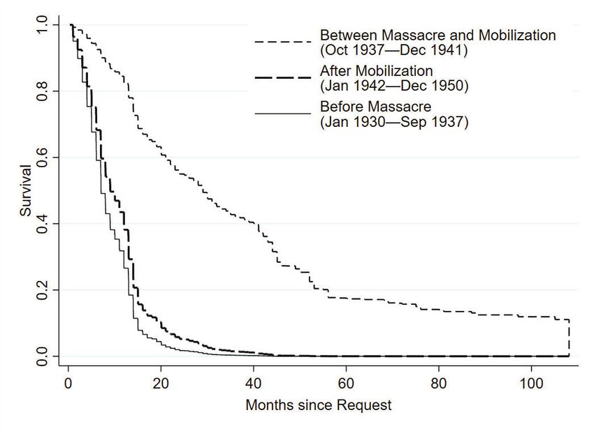
17Figure 4. Probability that property is still pending given the number of months since requested
Notes: Survival curves derived from a Cox proportional hazard model that controlled for property
type, the number of properties in the program’s queue at the time of the request, and dummy
variables for when the massacre and reform occurred.
18the processing time for requests. From the hazard model, we can derive survival curves (where
death means the property was processed) evaluated at three different points: before the massacre,
between the massacre and U.S. mobilization, and after U.S. mobilization.3 The three survival
curves are plotted in Figure 4. Note that a decrease in survival rates indicates the government is
processing requests faster, while an increase in survival rates indicates the government is struggling.
Before the massacre, the solid line indicates there was a 20% chance approval would take longer than
eight months. Between the massacre and U.S. mobilization, survival rates increased substantially.
The probability that approval would take longer than eight months increased to 85%, and there
was a 20% chance it would take longer than four years. But once external revenues dropped due
to U.S. mobilization, the curve returned to pre-massacre levels. The return to the pre-massacre
survival curve, even as more requests enter, suggests there might be an equilibrium level of state
capacity relative to the demands placed on it. The massacre moved the government away from this
equilibrium, but U.S. mobilization pushed the government to return to it.
The survival curves show the refugees strained the government’s capacity and that the external
revenue shock led to increased capacity. Before the refugees arrived, the government was in a
capacity-request equilibrium. But the refugee shock pushed the government out of the equilibrium
by flooding it with requests. Because the government did not expand capacity, delays increased.
But once World War II altered external revenues, the government invested in expanding capacity.
The government returned to the pre-refugee capacity-request equilibrium.
An additional piece of evidence that legal capacity increased after U.S. mobilization comes from
the demarcation of property. A key aspect of protecting property rights is demarcating the property
so that the state knows what it is protecting. While some countries demarcate properties through
geographic coordinates, the most common system is metes and bounds, which defines properties by
their local environment. HIRS used the metes and bounds system, defining properties by features
such as roads and, most commonly, by who occupied adjacent properties. The metes and bounds
system already suffers from worse property protections because of its dependence on local knowledge
and its vague definitions of property boundaries (Libecap and Lueck 2011). But, as Dimitruk et al.
(2021) show, the metes and bounds system can be even worse when low state capacity impedes a
proper demarcation of the property.
One of the main purposes of the Le Moniteur notifications was to demarcate properties. But
3
Note that these three points correspond to three combinations of dummy variables. Before the massacre, both
dummy variables equal zero. Between the massacre and the reform the massacre dummy equals 1 but the reform
dummy equals zero. And for after the reform both the massacre and reform dummies equal one.
19Figure 5. Proportion of property boundaries with incomplete demarcation, 1930-1949
Notes: A neighbor is unknown if the notification in Le Moniteur names the neighbor as “Qui de
droit” or “Whoever owns it.” Each property has four neighbors (one for each cardinal direction).
The gray area indicates the 95% confidence interval for proportion of neighbors who are unknown.
Confidence intervals come from a pooled regression with the proportion of unknown neighbors as
the dependent variable and year-dummies as the only explanatory variable.
throughout the notifications, we observe times when HIRS provided incomplete descriptions. The
most common incomplete description was to say that the adjacent property was occupied by “Qui
de droit,” that is, “Whoever owns it.” This could be an admission that the HIRS agent could
not find the property’s owner. But it also could indicate that the agent decided that the benefit
of finding the owner was not worth the effort. This decision, however, creates insecurity for the
tenant. Greater legal capacity, then, means more properties have complete demarcations.
Figure 5 shows the proportion of property boundaries with incomplete demarcation by request
year. Demarcation is incomplete if the boundary’s occupant is described as “Qui de droit,” and
each property has four boundaries. Figure 5 shows that before the massacre, between 1 and 2%
of boundaries were incompletely demarcated. After the massacre, we see this figure peak at 4%.
These properties, as seen in Figure 2, were the ones with the longest delay between request and
approval, providing further evidence that legal capacity was strained during this period. But after
U.S. mobilization, the proportion of incomplete boundaries rapidly decreases until it approaches
zero. Thus, not only did the state reduce processing delays after U.S. mobilization, it defined
20properties better, which should increase property right security. These are good indicators that
legal capacity increased.
The third piece of evidence in favor of greater legal capacity comes from rents collected on the
properties. Rental revenues can only increase if the state protects the property. One could object
and say that revenues increase if fiscal capacity increases. Indeed, we know from Table 3 that
the state was inefficient at collecting rents, and higher fiscal capacity should increase collection
efficiency. But for property, if the state tried to improve its efficiency by collecting rents without
protecting claims, the state would fail. That is because tenants were not obligated to remain on
the rental plots. If tenants felt that the rent they were paying did not justify the protections they
received, they could exercise their outside option and squat on unoccupied land. This is especially
true for refugees who had waited years to get their requests approved. Rental revenue could only
increase if the property was protected; i.e. if the state had sufficient legal capacity.
To see how U.S. mobilization affected rental revenues, we can use the fact that the rented
properties were disproportionately in areas with refugees. If legal capacity improved, then we would
expect rent collection to increase in these areas. To test this hypothesis, I compare rent collections
in tax precincts with and without refugees using a synthetic control analysis. The data on rent
collections are available only at the tax precinct level, of which there are ten in the country during
this period. Of those ten, only two hosted refugee camps (see Figure 1). Thus, the small sample size
makes a difference-in-differences approach difficult. Fortunately, a generalized version of difference-
in-differences is available in the synthetic control approach (Abadie et al. 2010). Synthetic control
and difference-in-differences are similar, except in difference-in-differences the analysis attributes
equal weight to all control observations whereas the synthetic control analysis weights control
observations to best match the treatment group. Although I focus on the results from the synthetic
control analysis, the Appendix contains the results from a difference-in-differences analysis and
compares them to the synthetic control, revealing similar results.
Because I have limited data, constructing the synthetic control is straightforward. The goal is to
compare rent collections in precincts with refugees (treated precincts) to precincts without refugees
(control precincts). Because the precincts are treated by the refugees before U.S. mobilization, I
use October 1937 as the treatment date. The analysis, then, will look at how the precincts behave
when the refugees arrive and if there was a change in 1942. The synthetic control weights are
estimated from taxes collected from October 1933 to September 1937. Receipts are transformed
with a logarithmic transformation and normalized to zero in 1937 (the financial year before the
21refugees arrived).
The synthetic control analysis shows that the refugees had a large and sustained impact on
public land rental receipts, and the effect was magnified by the U.S. mobilization’s effect on capacity.
Figure 6a plots the treatment and synthetic control. From 1933 to 1937, the two groups followed
similar patterns. But after 1937, the precincts diverged. Between the refugees’ arrival in 1938 and
mobilization at the end of 1941, rental revenues in refugee precincts were about 20% higher than
non-refugee precincts (p-values are significant and reported in Table A1). After U.S. mobilization,
refugee precincts increased yet again by about 20%, widening the gap between the two types. As
non-refugee districts collected more, the gap narrowed, but stayed large in 1949.
The evidence in Figure 6a is consistent with the U.S. mobilization increasing legal capacity.
But one factor that could confound the analysis is if there was a separate economic shock that also
increased land values and was coincident with both the timing of the reform and the location of
the refugees. For instance, U.S. mobilization may have increased demand for goods produced in
the refugee precincts, which subsequently increased land values. Such a concern is valid but fails
to explain why there are unmistakable shifts not just when the U.S. mobilized but also when the
refugees first came. Regardless, to address the concern, I do a placebo synthetic control analysis,
replacing the dependent variable with documentary recording fees; i.e. fees collected from recording
mortgages and property transfers. Looking at recording fees is a great placebo test because, like
the rental receipts, the fees are related to the value of land, but the refugees did not have the assets
to get mortgages or buy property. Thus, we should not see a difference between precincts.
Figure 6b displays the treatment and synthetic control units using property transfer receipts as
the dependent variable. The patterns in property transfer receipts are distinct from the patterns
found for land rental receipts. There were no shocks in recording fees that were unique to refugee
precincts, neither following the refugees’ entrance nor after U.S. mobilization. The post-1942 in-
crease affected all precincts equally. I address this increase in the next section.
The evidence makes a convincing case that legal capacity increased after U.S. mobilization.
After the drop in external revenues, the state processed requests quicker, provided a more complete
demarcation of property, and collected more rental revenues. All of this evidence runs counter to
the model, which said that the state should invest in legal capacity when external revenues are
high. What is more puzzling is that the state waited until 1942 to increase legal capacity even
though there was clear demand for greater legal capacity with the refugees’ arrival at the end of
1937 when customs revenues were 16% higher. Together, the evidence suggests that the model of
22Figure 6. The effect of refugees and U.S. mobilization on receipts from public land rentals, 1930-
1949
Notes: Figures display the treatment and synthetic control units. Panel (a) displays land rental
receipts, the variable of interest, and (b) shows property transfer receipts, the placebo. The dark
red line indicates when treatment was assigned in the synthetic control analysis (when the refugees
arrived). The light dashed line indicates the 1942 U.S. mobilization, though the analysis did nothing
to account for it.
23Figure 7. Budget, expenditures, and wages for the internal revenue service, 1930-1948
Notes: Data come from the Annual Reports of the Fiscal Representative.
investing in fiscal and legal capacity is incomplete.
6 Why Did Legal Capacity Increase?
The effect of U.S. mobilization on Haiti’s legal capacity suggests the model is missing key features
of how states invest in capacity. Using the institutional history of Haiti, I suggest two reasons why
the model is incomplete. I also examine their implications for other developing countries.
First, the model assumes that revenues from income tax and customs are fungible. But, at
least in Haiti, the appropriations law treated them differently. The appropriations law gave HIRS
15% of the government’s internal revenues (Banque nationale de la Republique d’Haiti 1942 p 15).
None of HIRS’s budget came from customs revenue. Table 1 shows that internal revenues were
relatively constant in the pre-reform period. As such, from 1934 to 1941, the nominal budget for
the IRS was flat, as shown in Figure 7. In that same figure, expenditures before 1942 are almost
indistinguishable from the budget because HIRS spent its entire allocation. This provides a partial
answer for why the state did not invest in legal capacity when the refugees started coming at the
end of 1937: HIRS was already spending all of its budget and could not make room for investing
in state capacity.
24Figure 8. Difference in delay between urban and rural properties before and after the massacre
Notes: Omitted month is three months after the massacre (January 1938). No agricultural prop-
erties were requested in November or December 1937 (1 and 2 months after the massacre).
We can test the budget constraint hypothesis by looking at property requested immediately
around the massacre. Refugees primarily demanded agricultural plots, which required more re-
sources to survey and appraise than urban properties: before 1938, the average delay for urban
properties was 4.7 months while agricultural properties had to wait 6.3 months. Comparing the ru-
ral and urban properties allows us to observe the immediate effect of refugees on delays. I estimate
the following regression
ln Delayit = βt (Agi × δt ) + δc + δt + εit (12)
where Delayit indicates the processing delay for property i in month t; Agi indicates whether
property i was an agricultural property; and δj and δt are district and time fixed effects. The
coefficient βt gives the difference in delays between agricultural and urban properties in month t.
The sample period is limited to requests made from November 1937 to October 1939, a two year
window centered on the massacre.
Figure 8 plots the βt s from the regression. The difference in delays between agricultural and
urban properties stays consistent through most of the surrounding months, except for an anomaly
for plots requested in the four months before the massacre. For such requests, delays for agricultural
25properties spiked: instead of waiting six months, tenants had to wait five years.
The pre-massacre spike in delays can be explained by the government diverting its limited
capacity to address the needs of the refugees. When the refugees arrived in October 1937, the
government was still processing plots requested in July, and it had few employees to administer
the program and survey properties. With constrained legal capacity, resources moved to where it
would provide the greatest value. The urgency of the refugee crisis required the government to
send its few employees to help with the requested plots. Thus, the non-refugee requests that were
still being processed were put on hold until the government could cover the refugees’ needs. The
timing of when these pre-massacre requests were finally fulfilled suggests that U.S. mobilization
triggered an investment in legal capacity. The government took five years to approve the shelved
requests, meaning they were finally addressed in 1942, just after U.S. mobilization. Only then was
legal capacity relaxed enough to reallocate resources to the low-priority requests.
This institutional understanding also explains why the government invested in legal capacity
after U.S. mobilization. The external revenue shock did not directly affect legal capacity. The
external revenue shock triggered the income tax reform, and income taxes were the largest source
of internal revenues. Since the program received 15% of internal revenues, the income tax reform
doubled the HIRS budget by 1944. As the budget expanded, so did expenditures. Prior to the
reform, expenditures were constrained by the budget. But after the reform, as seen in Figure 7,
the budget expanded so quickly that expenditures could not keep pace. This budget expansion is
how the government could afford to invest in legal capacity.
A second reason legal capacity increased after U.S. mobilization was because the same admin-
istration collected taxes and processed land rentals. Much of the increase in HIRS expenditures
seems to have gone towards improving fiscal capacity through personnel. Figure 7 shows HIRS
spent a significant share of its budget on wages, and that expenditures for wages increased after the
reform. When the government expanded personnel to collect income taxes, those same personnel
could be used to run the land rental program. This explains why revenues for registration fees
increased as seen in Figure 6b: more personnel were available to collect them.
This complementarity is similar to what we saw in preindustrial France when increased fiscal
capacity induced investments in legal capacity (Johnson and Koyama 2014), but the mechanism
here is more because of economies of scope. While this particular arrangement is unique to Haiti,
it highlights just one way in which the model’s generalizations can differ from institutional reality.
These institutional constraints are unique to Haiti, but do they have general lessons? If insti-
26tutional constraints tie investments in legal capacity to investments in fiscal capacity, then such
countries have to decide if the benefit of increasing legal capacity is worth the cost of investing
in fiscal capacity. A state might want to improve property rights by giving clearly defined titles
to land. But to support that program it levies a property tax. For individuals, is a title to land
worth paying a land tax? In some cases it could be, but in other cases the marginal gain from
protected property might not justify the loss in consumption. For the state, both titling property
and collecting a property tax require investing in legal and fiscal capacity, but it might avoid such
investments if the individual cannot even justify the trade-off.
7 Conclusion
This paper provides evidence that external revenues may indirectly impede investments in legal
capacity through their direct effect on limiting fiscal capacity. Rather than investing in legal
capacity when customs revenues were high, the Haitian government waited to invest in legal capacity
until after low customs revenues forced it to invest in fiscal capacity. The combined investment in
legal and fiscal capacity can be explained by institutional constraints and complementarity between
the two investments.
The results from Haiti prompt questions about the independence of investments in other con-
texts. One trouble investigating it further is that legal capacity is difficult to measure. Evidence
from France, one of the few places where we can measure both fiscal and legal capacity, suggests
that investments had to occur together (Johnson and Koyama 2014). Since many other Latin
American countries had a similar reliance on customs revenues, it could be promising to look at
such countries for further evidence.
Regarding Haitian history, this paper points to fruitful directions to pursue. The land rental
data show that HIRS improved its ability to process property requests, but we do not have concrete
details on how the program achieved this. HIRS likely used the new personnel to help with pro-
cessing, but administrative records could clarify the microfoundations of expanding state capacity.
27Figure A1. The Trujillo Massacre’s effect on land requests for districts within 20 km of a refugee
camp
Notes: The shaded area represent 95% confidence intervals.
A Appendix
A.1 Confirming refugee effect on property requests
Palsson (2021) shows the Trujillo refugees increased requests for government land rentals, but the
analysis was limited to only agricultural properties. Since this paper expands the sample to urban
and unknown properties, I repeat the difference-in-differences analysis. The treatment group in the
difference-in-differences analysis is districts that are close to a refugee camp (i.e., within 20 km).
The data are condensed into six-month periods, and the following regression estimated:
sinh−1 (Reqit ) = δi + βt Dit + εit (13)
where Reqit is the number of requests per 1,000 inhabitants in commune i in the six-month period
t, δi is a commune fixed effect, and δt is a period fixed effect. The Dit is an interaction between
treatment status (district is within 20 km of a refugee camp) and the six-month period t; hence,
the βt are the difference in requests between treatment and control districts in period t. The
coefficients are estimated for each period before and after the massacre to test for pre-treatment
28trends. Because in many years Reqit equals 0, the dependent variable is transformed using the
inverse hyperbolic sine, which is similar to the logarithmic transformation but evaluated at zero
(Burbidge et al. 1988). To account for serial correlation, standard errors are clustered at the
commune level. The results are plotted in Figure A1 and confirm (a) there were no pre-treatment
differences in request trends and (b) the refugees had a large, causal impact on requests.
A.2 Comparing Synthetic Control to Event Study
The synthetic control analysis presented in Section 4 provides convincing evidence that the refugees
and the capacity expansion had significant effects on tax revenues. But a weakness of the synthetic
control analysis is that researchers have some degrees of freedom in selecting the synthetic control.
To assuage concerns about researcher bias, I also estimate a difference-in-difference event study
and compare the estimated treatment effects to the synthetic control. To test for refugee effects on
tax receipts, I run the following regression
ln Tit = δi + δt + βt (Ref ugeei × δt ) + εit (14)
where Tit is, for tax precinct i in year t, the tax receipts from land rentals (though in other situations
below, the dependent variable will be taxes in other categories). The regression includes fixed effects
for the year (δi ) and the precinct (δt ). The Ref ugeei variable is an indicator for whether the tax
precinct hosted a refugee camp, and the βt gives, for year t, the difference in receipts between refugee
and non-refugee tax precincts. Because there are only 10 precincts, I obtain confidence intervals
for βt using the wild bootstrap-t methods described in Cameron et al. (2008) and implemented in
Stata by Judson Caskey.
29You can also read