SURPRISE! and When to Schedule It.
←
→
Page content transcription
If your browser does not render page correctly, please read the page content below
arXiv:2106.02851v1 [cs.MA] 5 Jun 2021

                                                         SURPRISE! and When to Schedule It.
                                            Zhihuan Huang∗1,2 , Shengwei Xu∗1,2,4 , You Shan3 , Yuxuan Lu1,2 , Yuqing
                                                    Kong†,‡1,2 , Tracy Xiao Liu§3 , and Grant Schoenebeck¶ 4
                                                         1 Departmentof Computer Science, Peking University
                                                   2 Center
                                                          on Frontiers of Computing Studies, Peking University
                                                  3 School of Economics and Management, Tsinghua University
                                                         4 School of Information, University of Michigan
                                            1 {zhihuan.huang, shengwei.xu, yx_lu, yuqing.kong}@pku.edu.cn
                                                               3 shany19@mails.tsinghua.edu.cn
                                                                 3 liuxiao@sem.tsinghua.edu.cn
                                                                       4 schoeneb@umich.edu

                                                                                   June 8, 2021

                                                                                      Abstract
                                                    Information flow measures, over the duration of a game, the audience’s belief of
                                                who will win, and thus can reflect the amount of surprise in a game. To quantify the
                                                relationship between information flow and audiences’ perceived quality, we conduct a
                                                case study where subjects watch one of the world’s biggest esports events, LOL S10.
                                                In addition to eliciting information flow, we also ask subjects to report their rating
                                                for each game. We find that the amount of surprise in the end of the game plays a
                                                dominant role in predicting the rating. This suggests the importance of incorporating
                                                when the surprise occurs, in addition to the amount of surprise, in perceived quality
                                                models. For content providers, it implies that everything else being equal, it is better
                                                for twists to be more likely to happen toward the end of a show rather than uniformly
                                                throughout.

                                        1       Introduction
                                        The live streaming industry has been burgeoning around the world in recent years. This
                                        includes live streaming games which, in turn, encompasses content like esports (e.g., League
                                        of Legends, Dota2, CS:GO, Apex Legends), sports games (e.g., football, tennis), and other
                                            ∗
                                             Equal contribution
                                            †
                                             Corresponding author
                                           ‡
                                             Supported by National Natural Science Foundation of China award number 62002001
                                           §
                                             Supported by the National Key Research and Development Program of China award num-
                                        ber 2018YFB1004503
                                           ¶
                                             Supported by (United States) National Science Foundation award number 2007256

                                                                                           1
games like chess, poker, and virtual casinos. Esports and its related brands occupy 24.2%
of the hours watched on Twitch.tv.1 About 609 million people spent over 5 billion hours
watching video game streams in 2016.2
    Despite the popularity of these live shows, their quality varies significantly. We hypoth-
esize an audience’s perceived quality for such live streamed content is, in part, derived from
the surprise in the content. One way to capture the effect of surprise is to solicit informa-
tion flow delivered from the show. Before the game commences, the audience might have an
imperfect idea of who will win. As the live game unfolds, the audience learns better about
who the winner is likely to be. In particular, the winner is clear by the time the game ends.
Information flow measures, over the duration of a game the audience’s belief of who will
win. Intuitively, the surprise, measures how much information flow fluctuates over time.
    A key challenge is to quantify the relationship between the audiences’ information flow
and audiences’ perceived quality. Prior studies either assume such relationship theoretically
[6] or use a statistical model to generate the theoretic information flow and indirectly mea-
sure audiences’ perceived quality (e.g., by audience size) [3, 18, 5]. We instead elicit data
directly from the audience to quantify the relationship and provide new insights for the
development of such perceived quality models. Specifically, we elicit audiences’ real-time
beliefs to compute the amount of surprise in a game. We then study the relationship both
between the amount of surprise and perceived quality and also the relationship between
when the surprise occurs and perceived quality.
    We design the Information Flow Elicitation Platform to collect the audiences’ continuous
beliefs and afterward ratings. Specifically, subjects watch live streaming games and update
their beliefs for the games’ outcomes as many times as they want. The platform monetarily
rewards agents for their information flow reports in such a way that more accurate reports
lead to higher payments. Subjects also rate the game quality afterwards.
    We use our platform to conduct a study targeting LOL S10.3

Summary of our results. We find that the second half of the game has a larger amount
of surprise compared to the first half and the amount of surprise at the end of the game has
the strongest impact on the subjects’ average ratings. Moreover, subjects’ average ratings
are significantly positively correlated with the games’ surprise amount. Interestingly, the
surprise amount in the first half of the game is negatively correlated with the average
ratings, while this correlation in the second half is positive. One conjecture is that subjects
overweight their watching experience in later time periods, which is not captured in prior
studies. In other words, our results suggest that the perceived quality model should consider
the time factor and the designers can use a better information revelation strategy such that
the game is more likely to have a twist near the end. Additionally, we conduct robustness
checks by considering alternative causes of perceived quality fluctuations, e.g., the favorite
(home) team wins, and the results are consistent.
   1
     https://www.pwc.de/en/technology-media-and-telecommunication/digital-trend-outlook-esport-
2020/media-broadcasts.html
   2
     Based on Nate Nead’s report https://investmentbank.com/esports-gaming-video-content/
   3 The 2020 League of Legends World Championship is the tenth world championship for League of

Legends, an esports tournament for the video game developed by Riot Games. It was held from 25 September
to 31 October in Shanghai, China. There were 74 rounds of games in total and each game lasts for 30 to
40 minutes.

                                                   2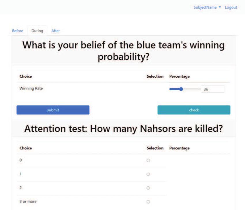
2 Belief Curves, Median Curves, and Surprise
In this section, we formally define the belief curve for each agent, and the aggregation
of agent’s beliefs into the information flow and median curve to compute the amount of
surprise in a game.
We focus on the two-team competition setting.
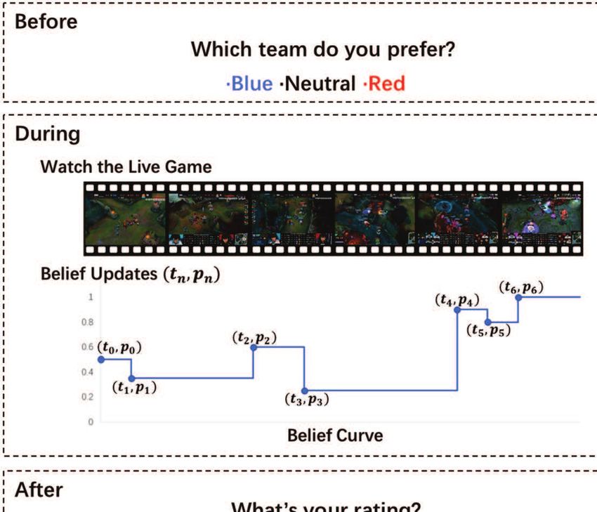
Belief curves and information flow. In game g, subject s has a sequence of belief
updates (the blue dots in Figure 2) chronologically {(t0 , p0 ), (t1 , p1 ), ..., (tn , pn )}, where n
is the number of times that subject s updates her belief in game g. Furthermore, t0 = startg
shows that she reports her prior belief p0 at the start of the game. Then she updates her
belief from p0 to p1 at time t1 and keeps updating her belief to the end. For convenience,
let tn+1 = endg . For all 0 ≤ i ≤ n, during period [ti , ti+1 ), subject s’s belief remains to be pi .
A subject s’s belief curve psg ∶ [startg , endg ) ↦ [0, 1] for a game g represents her continu-
ous belief throughout the game, where psg (t) is her belief for the winning probability of the
blue team at time t (Figure 2). The belief curve can be generated from her belief updates.
Formally,
Definition 2.1 (Belief curve). Subject s’s belief curve is psg ∶ [startg , endg ) ↦ [0, 1] where
psg (t) ∶= pi if t ∈ [ti , ti+1 ) for all 0 ≤ i ≤ n
The information flow is the collection of all the belief curves.
Median curve. To reduce the bias caused by irrational agents who always report extreme
beliefs (e.g., 0%, or 100%), we use the median curve to compute the surprise amount. See
Figure 1 for illustration of median curve and surprise amount.
Definition 2.2 (Median curve). For a game g which is watched by a set S of subjects,
we define median curve aSg ∶ [startg , endg ] ↦ [0, 1] as the median of the belief curve of all
subjects in S for game g, namely
∀t ∈ [startg , endg ], aSg (t) = median({psg (t)∣s ∈ S})
Figure 4 shows the median curves of three different games from our data set.
Surprise. Intuitively, if the median curve fluctuates severely, it suggests that this game
has a high degree of surprise. Following Ely et al. [6], we define the amount of surprise as
the sum of the change in the median curve.4 Formally,
Definition 2.3 (Surprise amount). Given a curve which is a step function in [x0 , xm+1 ]
f (t) = αi if t ∈ [xi , xi+1 ) for all 0 ≤ i ≤ m
We define the surprise amount of this curve as
m
Surp(f ) ∶= ∑ ∣αi+1 − αi ∣
i=0
4
This is seeming unrelated to the “surprisal score” sometimes used in Machine Learning.
3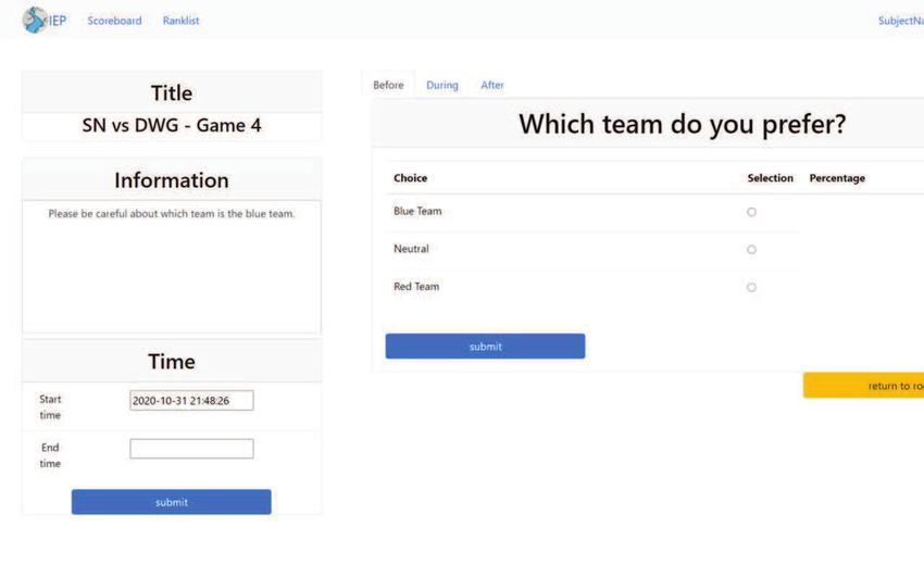
SurpSg ∶= Surp(aSg ) is the amount of surprise in game g, which is the sum of absolute
value of changes of the median curve aSg .5 We define aSg1 as aSg restricted to [startg , midg ]
and aSg2 as aSg restricted to [midg , endg ] where midg =
                                                          startg +endg
                                                                2
                                                                       . SurpSg1 ∶= Surp (aSg1 ) is
the amount of surprise in the first half of game g and Surpg2 ∶= Surp (aSg2 ) is the amount
                                                                S

of surprise in the second half of game g.

Figure 1: Surprise amount: we have three subjects s1 , s2 , s3 whose belief curves are green,
yellow and blue respectively. We aggregate their curves to a median curve which is the
median of subjects’ belief point wisely. The surprise amount is defined as the sum of
changes, which is ∣∆1 ∣ + ∣∆2 ∣.

Perceived quality vs. surprise. We estimate g’s perceived quality by its average rating
rgS over all subjects S who watch game g. To quantify the relationship both between the
amount of surprise and perceived quality and also study the relationship between when the
surprise occurs and perceived quality, we test the relationship between 1) game g’s surprise
amount SurpSg and its average rating rgS ; 2) game g’s surprise amount in the first half
SurpSg1 and rgS ; 3) game g’s surprise amount in the second half SurpSg2 and rgS .

3     Data Collection Methods
We first describe our Information Flow Elicitation Platform which was used to collect that
data. Second, we describe the data we collected.

3.1     Information Flow Elicitation Platform
A game is a competition between two teams, e.g., the red team vs. the blue team. For each
game, the study aims to collect three types of information from each subject: their team
preference, their real-time belief of the blue team’s winning probability, and their quality
rating for the game. Specifically, there are three stages for each game: before, during, and
after. Before the game, subjects report their preferences for the team. They also report
   5
     Since for all s ∈ S, psg (t) is a step function in [startg , endg ] of finite intervals, aS
                                                                                               g (t) is also a step
function in [startg , endg ] of finite intervals.

                                                        4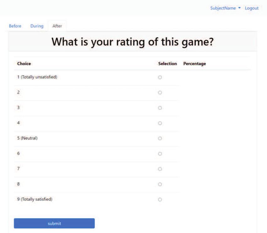
their prior belief for the blue team’s winning probability. During the game, subjects update
their real-time belief of the winning probability whenever they want. After the game, they
report their ratings for the game on a Likert scale, i.e., from 1 to 9, how much did you like
the game?

Figure 2: Workflow overview: we use a game in LOL S10 to illustrate the workflow. The
game is between two teams, blue and red. We ask subjects their team preference before the
game. Subjects view the game live and update their belief according to the game.6 After
the game, subjects rate the game.

Incentives. For each game, subjects receive a monetary reward which depends on their
overall prediction accuracy. To measure the overall prediction accuracy, we use the quadratic
scoring rule [4, 7] to measure the prediction accuracy at every t and integrate the quadratic

                                             5
(a) Before
(b) During (c) After
Figure 3: Screenshots of our platform: the above figures are subjects’ interface of our
platform.
6score over [startg , endg ].
Formally, each subject receives a score which depends on her belief curve. When the
game ends, the outcome og for the blue team is either 0 or 1. Subject s’s quadratic score
at time t is 1 − (psg (t) − og )2 . The overall quadratic score of subject s is:
1 endg
Score(psg ) = ∫ (1 − (psg (t) − og )2 )dt
endg − startg startg
For example, we consider a game where the starting time is 00:00, the ending time is
00:50, and the red team wins in the end. A subject reports her prior belief 40% for the
winning probability of the blue team at the beginning. Then she updates her belief to 80%
at 00:25, 50% at 00:30, and 0% at 00:40. Her score will be [(1 − 0.42 ) × (25 − 0) − (1 − 0.82) ×
(30 − 25) − (1 − 0.52 ) × (40 − 30) − (1 − 02 ) × (50 − 40)] × (1/50) = 0.86.
For subject s, at every time t, the expected quadratic score is maximized when psg (t)
is her true belief at time t. The expected score is maximized when ∀ t, psg (t) is her true
belief at time t. Thus, our score is incentive-compatible. However, this leads to non-fixed
cost. To fix the budget, following Lambert et al. [12], we calculate the average score over
all subjects in game g, Scoreg . Subject s’s reward is then
B
(1 + Score(psg ) − Scoreg )
Mg
where Mg denotes the number of subjects in game g. With the aforementioned reward, the
total reward for the game is fixed to B. Moreover, the reward is always non-negative and
has the same incentive properties as the original score.
3.2 Datasets
League of Legends. League of Legends is a free 5v5 online MOBA (multiplayer online
battle arena) game created and published by Riot Games. The goal of the teams is to
destroy the enemy team’s base. The match ends immediately after one teams’ base is
destroyed.
Data Properties. We use our platform to conduct a study for LOL S10 which consisted
of 76 individual games. We recruited 107 subjects from top Chinese universities. For each
game, a link to participate was sent out to all the participants. Subjects could participate
in as many or as few games as they like. Additionally, we did not restrict the number of
agents that signed up for each game.
We obtained 4,566 observations in total, where an observation consisted of one partic-
ular subject participating in one particular game. 5 subjects participated in all 76 games.
3 subjects of them only participate once. The average number of games that a subject
participated in was 42.67.
Exploratory Data Analysis. The average score for our subjects in each game was 0.817.
The average payment for our subjects in each game was 10.26 CNY (about $1.58 USD),
yielding a total payment of 46,850 CNY (about $7,230 USD).
6
The screenshots of the game is from LOL S10’s live streaming platform, https://www.bilibili.com/
7Average rating: 7.065 Rank: 12/76 Average rating: 4.564 Rank: 61/76 Average rating: 4.432 Rank: 64/76
100 100 100
80 80 80
60 60 60
belief(%)
belief(%)
belief(%)
40 40 40
20 20 20
0 0 0
0.0 0.2 0.4 0.6 0.8 1.0 0.0 0.2 0.4 0.6 0.8 1.0 0.0 0.2 0.4 0.6 0.8 1.0
time time time
(a) Likelihood that G2 beats SN (b) Likelihood that DWG beats (c) Likelihood that UOL beats
PSG DRX
Figure 4: Median curves of three games in LOL S10: the figures above shows the median
curves of three games with different ratings. The game in (a) has a very high rating:
rank 12 among all 76 games. This game is between two well matched teams. There are
several reversals in the game. The game in (b) has a low rating (rank 61/76); DWG is the
champion team, and PSG is a weak team. The subjects are confident that DWG will win
in the beginning, and the outcome fulfills their expectation. The game in (c) also has a low
rating (rank 64/76), UOL is slightly weaker than DRX. By the middle of the game, DRX
has taken control and the second half has no big surprises.
Moreover, the median frequency for belief updating is 5 and the average is 5.87. 68%
subjects are majoring in STEM. All subjects report that they have experience watching
LOL Live.
For each game, we can measure the number of subjects, the average rating, the duration,
the peak time, the surprise in the first half and the second half, the peak surprise, the end
surprise and the overall surprise. The peak time measures the most surprising time in the
game which we define as the middle of the time interval of 2.5 minutes that has the maximum
amount of surprise. The peak surprise is defined as the surprise amount generated in the
peak time. The end surprise is defined as the surprise amount generated in the last 2.5
minutes.
average min max
number of subjects 59.974 28 83
average rating 5.709 3.600 8.235
duration (min) 32.039 18.817 45.317
peak time (min) 23.950 2.600 44.042
1st half surprise 0.262 0.040 0.675
2nd half surprise 0.531 0.010 1.445
peak surprise 0.278 0.090 0.790
end surprise 0.162 0 0.725
overall surprise 0.793 0.150 1.750
Table 1: Summary statistics of our data
8Table 1 displays the average, minimum, and maximum of each of these quantities. Note
that on average, the surprise in the second half is twice the surprise in the first half.
30 30
25 25
20 20
count
count
15 15
10 10
5 5
0 0
20 30 40 50 60 70 1 3 5 7 9
number average rating
(a) The number of subjects in games (b) Average game rating
30 30
25 25
20 20
count
count
15 15
10 10
5 5
0 0
0 10 20 30 40 50 0 10 20 30 40 50
time(min) time(min)
(c) Length of the game (d) Time that peak occurs
Figure 5: Histogram of multiple statistics over all games: a) number of participating sub-
jects; b) the average ratings; c) duration d) the peak times (when surprise is the highest).
We also draw the kernel density estimation curve of these histograms.
Figure 5 shows a histogram of the first four of these quantities. Observe that the most
frequent peak times are between 20 to 30 minutes. This corresponds to a key part of the
matches, killing the first dragon (Baron Nashor), which appears exactly at the 20th minute
of the match, and is tyfiguresally killed between the 20 and 30 minute mark and grants the
successful team a lasting advantage.
91.5
8 0.8 8
2nd half surprise
7 0.6 7
end surprise
1.0
rating
rating
6 0.4 6
0.5 0.2
5 5
0.0
4 4
0.0
0.2 0.4 0.6 0.2 0.4 0.6
1st half surprise peak surprise
(a) First half vs. second half (b) Peak vs. end
Figure 6: Relationship between surprise in different time: Each point represents a game
and is colored by the game’s average rating. The figures also show the linear regression
lines.
Figure 6(a) shows a scatter plot of the surprise in the first half and second half of each
match. The points are colored by how exciting the match was, measured by the match’s
average rating. We can see that these values are negatively correlated. Figure 6(b) is a
scatter plot of the surprise in the peak time and end time of each match. These values are
positively correlated. We also find that peak is end for 19.7% games.
Figure 7 displays the amount of surprise over time. Short games, tend not to have too
much surprise, perhaps, because the teams are unevenly matched. Long games tend to start
off with less surprise, likely as the teams remain evenly matched, but have a substantial
amount of surprise toward the end.
4 Results
First, we analyze the relationship between the subjects’ ratings and the amount of surprise
in the game. We find that the average rating is significantly positively correlated with
the amount of surprise (Figure 8(a), Table 2, Column (1)). We further divide the game
into two halves and observe opposite effects between the two time windows. There is a
significantly positive correlation between the ratings and the surprise amount in the second
half (Figure 8(c), Table 2, Column (3)), while this correlation is negative in the first half
(Figure 8(b), Table 2, Column (2)). This result remains when we regress on both the first
half surprise and the second half surprise together (Figure 8(b), Table 2, Column (4)).
Importantly, the second half surprise better predicts the average rating than the overall
surprise: the coefficient value is 1.743 for second half surprise while it is 1.214 for the overall
surprise. Moreover, the adjusted R2 value is also greater when using second half surprise
than when using the overall surprise. One possibility is that subjects may overweight their
watching experiences in the second half of the game. Our result suggests that to optimize
the information revelation strategy, the optimization goal should consider time factors and
100.8
duration < 25 min
0.7 duration in 25 to 35 min
duration > 35 min
0.6
0.5
surprise
0.4
0.3
0.2
0.1
0.0
5 10 15 20 25 30 35 40 45
time(min)
Figure 7: Amount of surprise over time: We discretize time and, at each time, calculate
the surprise amount in the time interval of 2.5 minutes centered at that time. Each dot
in the figure represents the surprise amount in a certain game and a certain time interval.
The color of a dot shows the duration of the corresponding game. There are three colors in
total, red means the corresponding game lasts less than 25 minutes, green means it lasts 25
to 35 minutes, and blue means it lasts more than 35 minutes. The colored lines represent
the average surprise amount in games with the same color at a certain time.
emphasize the later surprise more.
A possible explanation for this result is the peak-end-effect [11, 2]. That is, people judge
an experience mostly based on how they felt at its peak, the most intense point, and at its
end, rather than based on the sum of their feeling at all moments of the experience. Thus,
we further analyze the effect of the peak surprise and the end surprise in our data (see
definition in Section 3.2). Our results show that both of them are highly correlated with
the average rating, while the end surprise has the highest correlation (see Table 3). Note
that the end surprise explains even more than the second half surprise (the end surprise’s
adjusted R2 value is 0.232 which is greater than the second half surprise’s adjusted R2 value
0.222).
Second, we observe a salient increase (decrease) in ratings for subjects whose preferred
team wins (loses). In a game with audiences whose preferences are homogeneous, e.g., a
popular team vs. an unpopular team, such individual rating biases lead to an unfairly
high (low) average rating for a game depending on the outcome of the game. Therefore, we
separate games into three categories: win, lose and neutral. The win (lose) category includes
games where the winning (losing) team was preferred by a majority of subjects. The neutral
category consists of games where neither team was preferred by the majority (recall that
11(1) (2) (3) (4)
Surprise 1.214∗∗∗
(0.399)
1st half -2.921∗∗∗ -2.100∗∗
surprise (0.911) (0.846)
2nd half 1.743∗∗∗ 1.533∗∗∗
surprise (0.368) (0.366)
Constant 4.746∗∗∗ 6.473∗∗∗ 4.783∗∗∗ 5.444∗∗∗
(0.340) (0.269) (0.227) (0.345)
N 76 76 76 76
adj. R2 0.099 0.110 0.222 0.273
Table 2: OLS regression of surprise and rating in different time periods. The dependent
variable is rating score. The independent variable in Columns (1), (2), (3) is surprise, 1st
half surprise, 2nd half surprise respectively, and the independent variable in Columns (4)
are the 1st half surprise and 2nd half surprise, together. The 1st and 2nd half surprise
indicates that the amount of surprise of the 1st and 2nd half of the game. The surprise
represents overall amount of surprise in the whole game. Standard errors are reported in
parentheses. ***, **, and * indicate statistical significance at the 1%, 5%, and 10% levels,
respectively.
(1) (2) (3)
Peak surprise 3.459∗∗∗ -0.582
(0.947) (1.637)
End surprise 3.146∗∗∗ 3.497∗∗∗
(0.647) (1.183)
Constant 4.746∗∗∗ 5.200∗∗∗ 5.304∗∗∗
(0.290) (0.156) (0.335)
N 76 76 76
adj. R2 0.141 0.232 0.223
Table 3: OLS regression of peak-end surprise and rating. The dependent variable is rating
score. The independent variable in Columns (1), (2) is peak surprise, end surprise, respec-
tively. The independent variables in Column (3) are peak surprise, end surprise, together.
The peak surprise indicates the amount of surprise in peak time. The end surprise indicates
the amount of surprise generated in the last 2.5 minutes. Standard errors are reported in
parentheses. ***, **, and * indicate statistical significance at the 1%, 5%, and 10% levels,
respectively.
subjects can also be neutral in their team preference). The results are in Figure 8(f) to 8(j)
and Table 4. Again, we observe similar results across all three categories of games.
In addition to the amount of surprise, we also explore other factors that may affect the
audience’s average rating.
Comeback size. It is defined as one minus the minimum winning probability of the winner
during the game. This feature characterizes how big the surprise of the outcome is.
12(1) (2) (3) (4)
all win game lose game neutral game
Surprise 1.692∗∗∗ 1.211∗∗∗ 2.088∗∗∗ 1.760∗∗∗
(0.293) (0.489) (0.557) (0.507)
Win 1.498∗∗∗
(0.198)
Lose -0.376
(0.232)
Constant 3.928∗∗∗ 5.783∗∗∗ 3.162∗∗∗ 3.879∗∗∗
(0.251) (0.389) (0.585) (0.385)
N 76 27 19 30
adj. R2 0.575 0.165 0.420 0.276
Table 4: OLS regression of surprise and rating in different games. Column (1) is the pooling
result. Column (2) refers to games where the majority preferred team wins. Column (3)
refers to games where the majority preferred team loses, and Column (4) is for games
where no team is preferred by the majority. The dependent variable is the rating score. The
independent variable in Column (1) is the amount of surprise, a dummy for winning (losing),
i.e., whether the game is won (lost) by the majority preferred team. The independent
variable in Columns (2), (3), (4) is the amount of surprise, respectively. Standard errors
are reported in parentheses. ***, **, and * indicate statistical significance at the 1%, 5%,
and 10% levels, respectively.
The coefficient value is 1.737 and the adjusted R2 value is 0.029.
Number of leader changes. It is defined as the number of times when the team with
more than 50% winning probability changes. This feature characterizes the team
with advantage changes. The coefficient value is −0.677 and the adjusted R2 value is
0.017.
Rubbish time. Given a threshold p, the rubbish time is defined as the proportion of time
period between the last time that the winner’s winning probability ≥ p and the end of
the match. p is a parameter from 0.5 to 1. This feature characterizes the unsurprising
time before the end. Intuitively, rubbish time is correlated with the end surprise and
negatively correlated with the rating. Our results show that p = 0.7 has the best
performance which has the coefficient value as −1.524 and the adjusted R2 value as
0.175.
Among the above three factors, the rubbish time is the most relevant factor but is still less
effective than the end surprise.
5 Related Work
Surprise vs. perceived quality. Starting from Ely et al. [6], a growing literature ex-
amines the relationship between the surprise and the perceived quality in different games,
such as tennis games [3], soccer games [5] and rugby games [18].
13Uncategorized
8 8 8 8 8
7 7 7 7 7
rating
rating
rating
rating
rating
6 6 6 6 6
5 5 5 5 5
4 4 4 4 4
0.0 0.5 1.0 1.5 0.0 0.5 1.0 1.5 0.0 0.5 1.0 1.5 0.0 0.5 1.0 1.5 0.0 0.5 1.0 1.5
surprise 1st half surprise 2nd half surprise peak surprise end surprise
(a) whole game (b) 1st half (c) 2nd half (d) peak time (e) end time
Categorized
8 8 8 8 8
7 7 7 7 7
rating
rating
rating
rating
rating
6 6 6 6 6
5 neutral 5 neutral 5 neutral 5 neutral 5 neutral
lose lose lose lose lose
4 win 4 win 4 win 4 win 4 win
0.0 0.5 1.0 1.5 0.0 0.5 1.0 1.5 0.0 0.5 1.0 1.5 0.0 0.5 1.0 1.5 0.0 0.5 1.0 1.5
surprise 1st half surprise 2nd half surprise peak surprise end surprise
(f) whole game (g) 1st half (h) 2nd half (i) peak time (j) end time
Figure 8: Relationship between surprise amount and rating: In the figures above, each
point represents a game and the y-axis is the average rating of the subjects. The x-axis
is the surprise amount of the whole game (a,f), the first half (b,g), the second half (c,h),
the peak time (d,i), and the end time (e,j) correspondingly. In the second row, the games
are classified into three categories. The red points represent the game won by the majority
preferred team, the blue dots is the game where the majority preferred team failed, and the
gray dots represent the game where no team is preferred by the majority (most of them are
neutral.). The second row analyses the relationship between surprise amount and rating
using data of only one category. The results are similar to the above row which suggests
the robustness of the conclusion.
However, instead of eliciting belief curves, this literature tyfiguresally constructs them
from existing data. For example, Bizzozero et al. [3] model the probability of a certain side
winning by explicitly using tennis’s scoring systems. Similarly, Buraimo et al. [5] use an in-
play model which additionally exploits the information on team strength which is embedded
in the pre-match odds. Buraimo et al. [5] and Scarf et al. [18] both use the Poisson model
to estimate the number of goals scored by the participating teams in order to calculate the
probability of the final outcome of the game. Lucas et al. [13] analyze the tweets during
the World Cup and use the emotional changes to measure the surprise. In contrast to these
studies which estimate surprise using statistical models, our study measures the perceived
surprise amount by dynamically eliciting subjects’ beliefs.
These works also use different proxies for perceived quality. Buraimo et al. [5] analyze
the relationship between surprise and the real-time audience size for both halves of soccer
games. Instead, we focus on the relationship between surprise and the overall rating. Thus,
prior studies do not observe how the timing effects of surprise affect perceived quality.
In addition to surprise, massive literature also studies suspense, which is defined as
14how much the belief curve is expected to move in the very near future. Since measuring
suspense requires the ability to predict what might happen in the near future, the analysis
for suspense is beyond the scope of the paper. In the future, it might be possible to learn
a model from the data which enables the analysis of suspense.
Prediction markets and polls. Prediction markets are designed to elicit continuously
updated forecasts about uncertain events. Prior studies have proved that prediction market
can outperform internal sales projections [15], journalists’ forecasts of Oscar winners [14],
and expert economic forecasters [9].
In prediction polls, forecasters express their beliefs by answering questions like "how
likely is this event?". In both prediction markets and polls, forecasters can update their
predictions whenever they wish. In contrast to prediction markets, in prediction polls,
forecasters update their predictions individually. Rothschild and Wolfers [17]’s work shows
that using prediction polls in elections can achieve better accuracy than opinion polls.
A few studies have compared the performance of prediction markets and polls, though
there is no conclusive answer [8, 16, 1]. Both Goel et al. [8] and Rieg and Schoder [16]
find no significant differences between these two methods. Atanasov et al. [1] find that the
aggregation rules in prediction polls affect its accuracy level. For example, simply averaging
all polls performs worse than a prediction market, while weighting the polls properly leads
to a better performance than a prediction market. Our elicitation method is more similar
to prediction polls.
6 Conclusion
We study the relationship between a game’s surprise amount and its perceived quality. We
develop a platform that collects audiences’ real-time beliefs and ratings of the LOL S10.
Our empirical analysis suggests that the level of surprise in the later time of a game has a
stronger impact on subjects’ ratings. This indicates that the audience would prefer surprise
to occur in the end of a game. A future direction is to define a new perceived quality model
that considers time factors and theoretically analyze the optimal way to reveal information
over time in this model. Future work could similarly optimize suspense.
Moreover, we expect that belief polls could be embedded in live streaming games as an
entertainment feature. Last but not least, we can collect other information such as the text
in bullet comments to better construct the information flow.
Acknowledgments
We would like to thank our anonymous reviewers for their insightful suggestions which
substantially improved the paper. We also thank Kening Ren, Jialun Yang, Xinlun Zhang,
Fan Yan and Zheng Zhong for their help and useful discussions. Finally, we thank our
participants in our LOL S10 study for their time, attention and effort. Some of the figures
are generated with Python Matplotlib [10].
15References
[1] Pavel Atanasov, Phillip Rescober, Eric Stone, Samuel A Swift, Emile Servan-Schreiber,
Philip Tetlock, Lyle Ungar, and Barbara Mellers. Distilling the wisdom of crowds:
Prediction markets vs. prediction polls. Management Science, 63(3):691–706, 2017.
[2] Alan D Baddeley and Graham Hitch. The recency effect: Implicit learning with explicit
retrieval? Memory & Cognition, 21(2):146–155, 1993.
[3] Paolo Bizzozero, Raphael Flepp, and Egon Franck. The importance of suspense and
surprise in entertainment demand: Evidence from wimbledon. Journal of Economic
Behavior & Organization, 130:47–63, 2016.
[4] G. W. Brier. Verification of forecasts expressed in terms of probability. Monthly
Weather Review, 78:1–3, 1950.
[5] Babatunde Buraimo, David Forrest, Ian G McHale, and JD Tena. Unscripted drama:
soccer audience response to suspense, surprise, and shock. Economic Inquiry, 58(2):
881–896, 2020.
[6] Jeffrey Ely, Alexander Frankel, and Emir Kamenica. Suspense and surprise. Journal
of Political Economy, 123(1):215–260, 2015.
[7] Tilmann Gneiting and Adrian Raftery. Strictly proper scoring rules, prediction, and
estimation. Journal of the American Statistical Association, 102:359–378, 03 2007. doi:
10.1198/016214506000001437.
[8] Sharad Goel, Daniel M Reeves, Duncan J Watts, and David M Pennock. Prediction
without markets. In Proceedings of the 11th ACM conference on Electronic commerce,
pages 357–366, 2010.
[9] Refet Gurkaynak and Justin Wolfers. Macroeconomic derivatives: An initial analysis
of market-based macro forecasts, uncertainty, and risk. Technical report, National
Bureau of Economic Research, 2006.
[10] J. D. Hunter. Matplotlib: A 2d graphics environment. Computing in Science & Engi-
neering, 9(3):90–95, 2007. doi: 10.1109/MCSE.2007.55.
[11] Daniel Kahneman, Barbara L Fredrickson, Charles A Schreiber, and Donald A Re-
delmeier. When more pain is preferred to less: Adding a better end. Psychological
science, 4(6):401–405, 1993.
[12] Nicolas S. Lambert, John Langford, Jennifer Wortman Vaughan, Yiling Chen,
Daniel M. Reeves, Yoav Shoham, and David M. Pennock. An axiomatic char-
acterization of wagering mechanisms. Journal of Economic Theory, 156:389 –
416, 2015. ISSN 0022-0531. doi: https://doi.org/10.1016/j.jet.2014.03.012. URL
http://www.sciencedirect.com/science/article/pii/S0022053114000520. Com-
puter Science and Economic Theory.
16[13] Gale M. Lucas, Jonathan Gratch, Nikolaos Malandrakis, Evan Szablowski, Eli
Fessler, and Jeffrey Nichols. Goaalll!: Using sentiment in the world cup to
explore theories of emotion. Image and Vision Computing, 65:58–65, 2017.
ISSN 0262-8856. doi: https://doi.org/10.1016/j.imavis.2017.01.006. URL
https://www.sciencedirect.com/science/article/pii/S0262885617300148.
Multimodal Sentiment Analysis and Mining in the Wild Image and Vision Computing.
[14] David M Pennock, Steve Lawrence, Finn Årup Nielsen, and C Lee Giles. Extracting
collective probabilistic forecasts from web games. In Proceedings of the seventh ACM
SIGKDD international conference on Knowledge discovery and data mining, pages 174–
183, 2001.
[15] Charles R Plott and Kay-Yut Chen. Information aggregation mechanisms: Concept,
design and implementation for a sales forecasting problem. Working paper No. 1131,
California Institute of Technology, Division of the Humanities and Social Sciences,
2002.
[16] Robert Rieg and Ramona Schoder. Forecasting accuracy: Comparing prediction mar-
kets and surveys-an experimental study. Journal of Prediction Markets, 4(3), 2010.
[17] David Rothschild and Justin Wolfers. Forecasting elections: Voter intentions versus
expectations. Available at SSRN 1884644, 2011.
[18] Phil Scarf, Rishikesh Parma, and Ian McHale. On outcome uncertainty and scoring
rates in sport: The case of international rugby union. European Journal of Operational
Research, 273(2):721–730, 2019.
17You can also read