SWIRL: A Sequential Windowed Inverse Reinforcement Learning Algorithm for Robot Tasks With Delayed Rewards - Stanford University
←
→
Page content transcription
If your browser does not render page correctly, please read the page content below
Journal Title
                                                                                                   XX(X):1–18
SWIRL: A Sequential Windowed Inverse                                                               ©The Author(s) 0000
                                                                                                   Reprints and permission:
Reinforcement Learning Algorithm for                                                               sagepub.co.uk/journalsPermissions.nav
                                                                                                   DOI: 10.1177/ToBeAssigned

Robot Tasks With Delayed Rewards                                                                   www.sagepub.com/

Sanjay Krishnan1 , Animesh Garg1,3 , Richard Liaw1 , Brijen Thananjeyan1 ,
Lauren Miller1 , Florian T. Pokorny2 , Ken Goldberg1

Abstract
We present Sequential Windowed Inverse Reinforcement Learning (SWIRL), a three-phase algorithm that automatically
partitions a task into shorter-horizon sub-tasks based on transitions that occur consistently across demonstrations.
SWIRL then learns a sequence of local reward functions using Maximum Entropy Inverse Reinforcement Learning.
Once these reward functions are learned, SWIRL applies Q-learning to compute a policy that maximizes the rewards.
SWIRL leverages both expert demonstrations and exploration to find policies for robotic tasks with delayed rewards.
Experiments suggest that SWIRL requires significantly fewer rollouts than pure RL and fewer expert demonstrations
than behavioral cloning to learn a policy. We evaluate SWIRL in two simulated control tasks, parallel parking and a
two-link pendulum. On the parallel parking task, SWIRL achieves the maximum reward on the task with 85% fewer
rollouts than Q-Learning, and 33% fewer rollouts than Q-Learning where the rewards were shaped by IRL. We also
consider physical experiments on surgical tensioning and cutting deformable sheets using the da Vinci surgical robot.
On the deformable tensioning task, SWIRL achieves a 36% relative improvement in reward compared to a baseline of
behavioral cloning with segmentation.

1     Introduction                                                et al. 2014). Often these segments are manually designed or
                                                                  derived from a dictionary of motion primitives, but recently,
An important problem in robot learning is defining a reward       there are several approaches for learning segmentation
function that accurately reflects a robot’s ability to perform    criteria automatically by identifying locally similar structure
a task. However, in many cases, the natural reward function       in demonstration data (Barbič et al. 2004; Chiappa and
for a task is delayed, where the consequences of an action are    Peters 2010; Alvarez et al. 2010; Calinon et al. 2010; Krüger
only observed long after it is taken. Such reward functions       et al. 2012; Niekum et al. 2012; Wächter and Asfour 2015;
are difficult to directly optimize with exploration-based         Lee et al. 2015). While prior work has mostly considered
techniques like Reinforcement Learning (RL). For example,         segmentation to reduce the complexity of deterministic
in a multi-step assembly task, one might have a classifier that   planning problems, this paper explores how segmentation
can determine if the full part is correctly assembled. In this    can inform reward derivation in the Markov Decision Process
problem, RL would have to rely on random exploration to           setting.
achieve the assembled state by chance at least once, before it       We model a task as a sequence of quadratic reward
can learn a more efficient policy.                                functions Rseq = [R1 , ..., Rk ] and transition regions G =
  One approach is to use expert demonstrations to learn           [ρ1 , ..., ρk ] such that R1 is the reward function until ρ1
a smoother reward function that gives the robot a stronger        is reached, after which R2 becomes the reward and so
reward signal at intermediate steps. This idea is related to      on. We assume that we have access to a supervisor that
apprenticeship learning (Kolter et al. 2007a; Coates et al.       provides demonstrations that are optimal w.r.t an unknown
2008; Abbeel and Ng 2004). In apprenticeship learning, a          Rseq , and reach each ρ ∈ G (also unknown) in the same
supervisor provides a small number of initial demonstrations,     sequence. Sequential Windowed Inverse Reinforcement
and there is a two-phase approach that first applies Inverse      Learning (SWIRL) is an algorithm to recover Rseq and
Reinforcement Learning (IRL) to infer the supervisor’s            G from the demonstration trajectories. SWIRL applies
implicit reward function, and then optimizes for this reward      to tasks with a discrete or continuous state-space and a
function using RL. We explore whether we can leverage             discrete action-space. The state space can represent spatial,
the same basic apprenticeship learning framework to learn         kinematic, or sensory states (e.g., visual features), as long as
reward functions for tasks with a sequence of state-space
sub-goals that must be reached.
                                                                  1
   Segmentation is a well-studied problem, and it facilitates       AUTOLAB, UC Berkeley automation.berkeley.edu
                                                                  2
learning localized control policies (Murali* et al. 2015;           RPL/CSC, KTH Royal Institute of Technology, Stockholm, Sweden
                                                                  3
                                                                    Stanford University
Niekum et al. 2012; Konidaris et al. 2011), adaptation to
unseen scenarios (Ijspeert et al. 2002; Ude et al. 2010),         Corresponding author:
and demonstrator skill-assessment (Reiley et al. 2010; Gao        Sanjay Krishnan sanjay@eecs.berkeley.edu

Prepared using sagej.cls [Version: 2016/06/24 v1.10]
2                                                                                                           Journal Title XX(X)

the trajectories are smooth and not very high-dimensional.               one such algorithm, and we describe extensions that
The discrete actions are not a fundamental restriction, but              account for non-linearities and discontinuities. For this
relaxing that constraint is deferred to future work. Finally,            class of segmentation algorithms, policy learning can
Rseq and G can be used in an RL algorithm to find an optimal             be efficiently done on an augmented state-space with
policy for a task.                                                       indicators tracking the previously reached segments.
   SWIRL segments the demonstrations using a variant
of a segmentation algorithm proposed in our prior                     3. We apply SWIRL to two simulated control tasks, a
work (Krishnan* et al. 2015; Murali* et al. 2016), called                noisy non-holonomic car and a two-link pendulum,
Transition State Clustering (TSC). TSC identifies locally                and two physical experiments on the da Vinci surgical
similar dynamical segments in a trajectory and fits a                    robot.
Gaussian Mixture Model to the endpoints of the segments
to learn a model to determine when and where a segment
terminates. While our original motivation was to improve          2    Related Work and Background
the robustness of kinematic segmentation algorithms by
pruning sparse clusters, TSC can also be interpreted as           Apprenticeship Learning:         Abbeel and Ng (2004)
inferring the subtask transition regions G. SWIRL extends         argue that the reward function is often a more concise
TSC by (1) formalizing a broader class of Markov                  representation of task than a policy. As such, a concise
segmentation algorithms that apply to the IRL setting where       reward function is more likely to be robust to small
TSC is a special case, and (2) combining TSC with a               perturbations in the task description. The downside is that
kernel embedding to handle certain types of non-linearities       the reward function is not useful on its own, and ultimately
and discontinuities in the state-space. Once the segments         a policy must be retrieved. In the most general case, an
are found, SWIRL applies Maximum Entropy Inverse                  RL algorithm must be used to optimize for that reward
Reinforcement Learning (MaxEnt-IRL) (Ziebart et al. 2008)         function (Abbeel and Ng 2004). It is well-established that
to each segment to find Rseq . Segmentation further simplifies    RL problems often converge slowly in complex tasks when
the estimation of dynamics models, which are required             rewards are sparse and not “shaped” appropriately (Ng et al.
for inference in MaxEnt-IRL, since locally many complex           1999; Judah et al. 2014). Our work re-visits this two-phase
systems can be approximated linearly in a short time horizon.     algorithm in the context of sequential tasks and techniques
   Learning a policy from Rseq and G is nontrivial because        to scale such an approach to longer time horizons. Related
solving k independent problems neglects any shared structure      to SWIRL, Kolter et al. studied Hierarchical Apprenticeship
in the value function during the policy learning phase (e.g.,     Learning to learn bipedal locomotion (Kolter et al. 2007a),
a common failure state). Jointly learning over all segments       where the algorithm is provided with a hierarchy sub-
introduces a dependence on history, namely, any policy            tasks. We explore automatically inferring a sequential task
must complete step i before step i + 1. Learning a memory-        structure from data.
dependent policy could lead to an exponential overhead of         Motion Primitives: The LfD and planning communities
additional states. SWIRL exploits the fact that TSC is a          studied the problem of leveraging motion primitives,
Markov segmentation algorithm and shows that the problem          or libraries of temporally extended action sequences,
can be posed as a proper MDP in a lifted state-space that         to improve generalization. Dynamic Motion Primitives
includes an indicator variable of the highest-index {1, ..., k}   construct new motions through a composition of dynamical
transition region that has been reached so far.                   building blocks (Ijspeert et al. 2002; Pastor et al. 2009;
   The basic model follows from a special case of                 Manschitz et al. 2015). Much of the work in motion
Hierarchical Reinforcement Learning (Sutton et al. 1999).         primitives considered manually identified segments, but
In hierarchical reinforcement learning, multi-step skills are     recently, Niekum et al. (Niekum et al. 2012) proposed
composed of local policies called “options”. Each option          learning the set of primitives from demonstrations using the
executes until a termination condition, and a meta-policy         Beta-Process Autoregressive Hidden Markov Model (BP-
selects the next option to execute. SWIRL is an IRL               AR-HMM). Similarly, Calinon (2014) proposed the task-
framework for inferring termination conditions (G) and local      parametrized movement model with GMMs for automatic
reward functions that guide the agent to these termination        action segmentation. Both Niekum and Calinon considered
states Rseq , where the meta-policy is deterministic and          the motion planning setting in which analytical planning
sequential.                                                       methods are used to solve a task. To the best of our
   In summary, our contributions are:                             knowledge, SWIRL is the first to consider segmentation in
                                                                  the IRL setting, where the dynamics can be stochastic.
    1. We describe a model for sequential robot tasks, where
       rewards sequentially switch upon arrival in a transition   Segmentation: Trajectory segmentation is a well-studied
       region, and an IRL algorithm called Sequential             area of research dating back to early biomechanics and
       Windowed Inverse Reinforcement Learning to infer           robotics research. For example, Viviani and Cenzato (1985)
       the rewards and transitions from demonstrations. The       explored using the “two-thirds” power law coefficient to
       algorithm has three phases: segmentation, inverse          determine segment boundaries in handwriting. Morasso
       reinforcement learning, and policy learning.               (1983) showed that rhythmic 3d motions of a human arm
                                                                  could be modeled as piecewise linear. In a seminal paper,
    2. We describe a class of segmentation algorithms,            Sternad and Schaal (1999) provided a formal framework
       Markov segmentation algorithms, which can be used          for control-theoretic segmentation of trajectories. Botvinick
       to partition a task. Transition State Clustering is        et al. (2009) explored the reinforcement learning analog

Prepared using sagej.cls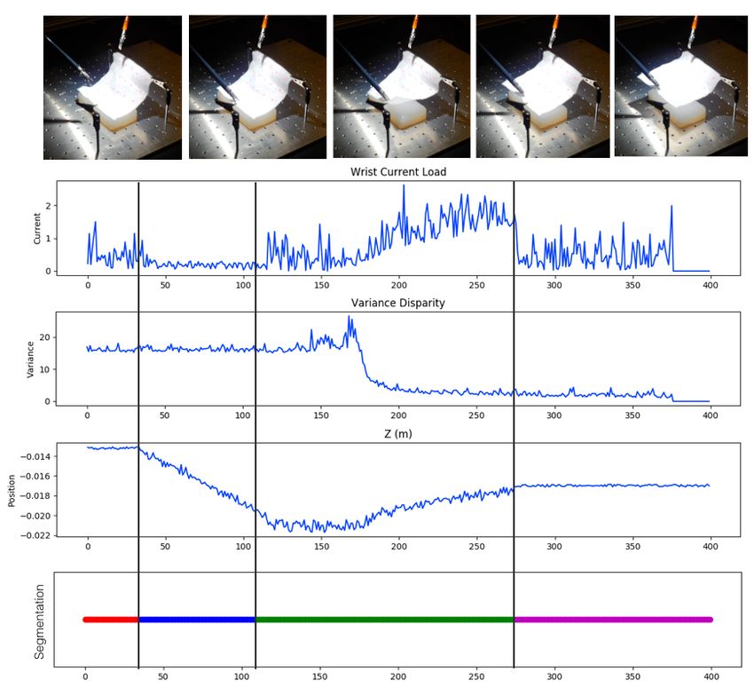
3

of the control-theoretic models. Concurrently, temporal-           S × A 7→ R. Associated with each Ri is a transition region
segmentation was developing in the motion capture                  ρi ⊆ S, which is a subset of the state-space. Each trajectory
community (Moeslund and Granum 2001). Recently,                    accumulates a reward Ri until it reaches the transition ρi ,
some Bayesian approaches have been proposed for the                then the robot switches to the next reward and transition pair.
segmentation problem (Asfour et al. 2006; Calinon and              This process continues until ρk is reached. A robot is deemed
Billard 2004; Kruger et al. 2010; Vakanski et al. 2012;            successful when all of the ρi ∈ G are reached in sequence.
Tanwani and Calinon 2016). One challenge is collecting                Inverse Reinforcement Learning (IRL) Ng and Russell
enough data to employ these techniques and tuning the              (2000) describes the problem of observing an agent’s
hyperparameters. In prior work, we observed that under             behavior and inferring a reward function that best explains
the assumption that the task is sequential (same order of          the agent’s actions (assuming the agent is behaving
primitives in each demonstration) the inference could be           optimally). Let D = {di } be a set of demonstrations of a
modeled as a two-level clustering problem (Krishnan* et al.        robotic task. Each demonstration of a task d is a discrete-time
2015). This results in improved accuracy and robustness for        sequence of T feature vectors. In this paper, we consider the
a small number of demonstrations. Another relevant result is       sequential version of this problem, where we have to infer k
from Ranchod et al. (2015), who use an IRL model to define         reward functions and k transition regions.
the primitives, in contrast to the problem of learning a policy
                                                                   Sequential IRL Problem: Given observations of a
after IRL.
                                                                   successful robot through a set of demonstration trajectories
Hierarchical Reinforcement Learning: The field of hier-            D = {d1 , ..., dk }, infer Rseq and G.
archical reinforcement learning has a long history (Sutton
et al. 1999; Barto and Mahadevan 2003) in AI and in the               Most IRL algorithms implicitly learn an optimal policy.
analysis of biological systems (Botvinick 2008; Botvinick          However, the dynamics of the demonstration environment
et al. 2009; Solway et al. 2014; Zacks et al. 2011; Whiten         can differ from the dynamics of the execution environment
et al. 2006). Early work in hierarchical control demonstrated      in unknown ways–and the rewards might transfer but the
the advantages of hierarchical structures by handcrafting hi-      policies might not. Furthermore, we observed that in practice
erarchical policies (Brooks 1986) and by learning them given       the reward function is often more concise than the policy and
various manual specifications: state abstractions (Dayan and       more tolerant to estimation errors. If we have only observed
Hinton 1992; Hengst 2002; Kolter et al. 2007b; Konidaris           a small number of demonstrations, one might have enough
and Barto 2007), a set of waypoints (Kaelbling 1993), low-         data to learn a reasonable reward function but not a viable
level skills (Huber and Grupen 1997; Bacon and Precup              policy. Therefore, after learning Rseq and G, there needs to
2015), a set of finite-state meta-controllers (Parr and Russell    be a policy learning phase. In the most general case, we will
1997), a set of subgoals (Sutton et al. 1999; Dietterich 2000),    have to apply a technique like RL to learn a policy.
or intrinsic reward (Kulkarni et al. 2016). The key abstraction    Sequential RL: Given a new instance, Rseq , and G, learn an
used in hierarchical RL is the “options” framework, where          optimal policy π ∗ .
sub-skills are represented by local policies, termination con-
ditions, and initialization conditions. A high-level policy
switches between these options and composes them into a            3.2    Modeling Assumptions
larger task policy. In this framework, per sub-skill reward        To make these problem statements more formal and compu-
functions are called sub-goals. SWIRL is an algorithm to           tationally tractable, we make some modeling assumptions.
learn quadratic sub-goals and termination conditions, where
the high-level policy is deterministic and sequentially iterates   Assumption 1. Reward Transitions are Identifiable: The
through the sub-skills.                                            key challenge in this problem is determining when a
                                                                   transition occurs–identifying the points in time in each
                                                                   trajectory at which the robot reaches a ρi and transitions
3     Model and Problem Statement                                  the reward function. The natural first question is whether
3.1      Basic Setup                                               this is identifiable, that is, whether it is even theoretically
                                                                   possible to determine whether a transition ρi → ρi+1 has
Consider a finite-horizon Markov Decision Process (MDP):
                                                                   occurred after obtaining an infinite number of observations.
                           M = hS, A, P(·, ·), R, T i,             Trivially, this is not guaranteed when Ri+1 = Ri , where it
                                                                   would be impossible to identify a transition purely from
where S is the set of states (continuous or discrete), A is
                                                                   the supervisor’s behavior (i.e., no change in reward, implies
the set of actions (finite and discrete), P : S × A 7→ Pr(S)
                                                                   no change in behavior). Perhaps surprisingly, this is still
is the dynamics model that maps states and actions to a
                                                                   not guaranteed even if Ri+1 6= Ri due to policy invariance
probability density over subsequent states, T is the time-
                                                                   classes Ng et al. (1999). Consider a reward function Ri+1 =
horizon, and R is a reward function that maps trajectories
                                                                   2Ri , which functionally induce the same optimal behavior.
of length T to scalar values. At every state s, we also observe
                                                                   Therefore, we consider a setting where all of the rewards in
a vector of perceptual features x ∈ X . The feature space
                                                                   Rseq are distinct and are not equivalent w.r.t optimal policies.
can be a concatenation of kinematic features Xk (e.g., robot
                                                                   There are known necessary and sufficient conditions, see
position) and sensory features Xs (e.g., visual features from
                                                                   Theorem 1 in Ng et al. (1999).
the environment). We assume that this feature space is low-
dimensional.                                                       Assumption 2. Myopic Optimality: Next, to be able
   Sequential tasks are tasks defined in terms of a sequence       to infer the reward function we have to assume that the
of reward functions, Rseq = [R1 , ..., Rk ], where each Ri :       supervisor is behaving optimally. However, in the sequential

Prepared using sagej.cls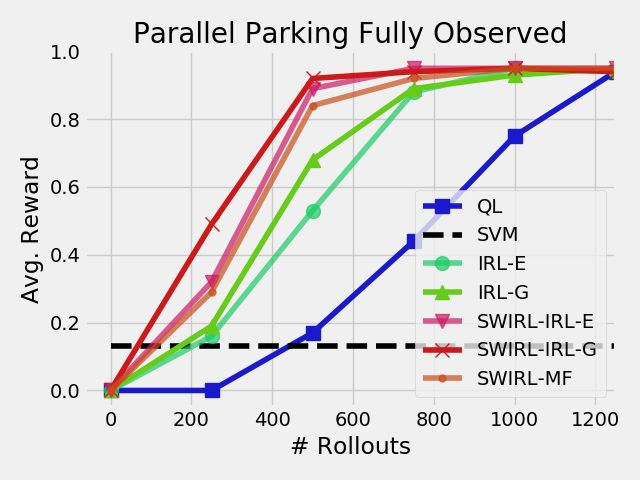
4                                                                                                              Journal Title XX(X)

problem, the globally optimal solution (maximizes the                During the online phase (Policy Learning), the algorithm
cumulative reward of all sub-tasks) is not necessarily locally    only observes the partial trajectory up to the current time-step
optimal. For example, it might be advantageous to be sub-         and does not observe which segment is active. In this sense,
optimal in an earlier sub-task if it leads to a much higher       segmentation introduces a problem of partial observation
reward in a later sub-task. We make the assumption that the       even if the original task is fully observed. The segmentation
supervisor’s behavior is myopic, i.e., the supervisor applies     needs to be estimated from the history of the process.
the optimal stationary policy with respect to its current            Trivially, some algorithms are not applicable since they
reward function ignoring all future rewards.                      might require knowledge of future data (e.g., a forward-
                                                                  backward HMM algorithm). Even if the algorithm is causal,
Assumption 3. Successful Demonstrations: We also need
                                                                  it might have an arbitrary dependence on the past leading
conditions on the demonstrations to be able to infer G. We
                                                                  to inefficient estimation of the currently active segment. To
assume that all demonstrations are successful, that is, they
                                                                  address this problem, we formalize the following condition:
visit each ρi ∈ G in the same sequence.
Assumption 4. Quadratic Rewards: We assume that each              Definition 1. Segmentation. A segmentation of a task is
reward function Ri can be expressed as a quadratic of the         a function F that maps every state-time tuple to an index
form (x − x0 )T Q(x − x0 ) for some positive semi-definite Q,     {1, ..., k}:
some feature vector x that is a function of the current state,                     F : X × Z+ 7→ {1, ..., k}
and a center point x0 with x0T Qx0 = 0. This means that for          A Markov segmentation function is a task segmentation
a d-dimensional feature space there are O(kd 2 ) parameters       where the segmentation index of time t + 1 can be completely
that describe the reward function.                                determined by the featurized state xt at time t and the index
Assumption 5. Ellipsoidal Approximation: Finally, we              it at time t:
assume that the transition regions in G can be approximated                             it+1 = M(xt , it )
by a set of disjoint ellipsoids over the perceptual features.
                                                                  4.2    General Framework
3.3      Algorithm Description                                    We now describe a general framework that takes a
Let D be a set of demonstration trajectories {d1 , ..., dN } of   segmentation algorithm and extracts a Markov segmentation
a task with a delayed reward. SWIRL can be described in           criteria. Suppose, we are given a function that does the
terms of three sub-algorithms:                                    following:
Inputs: Demonstrations D                                          Definition 2. Transition Indicator Function. A transition
1. Sequence Learning: Given D, SWIRL segments the task            indicator function T is a function that maps each featurized
   into k sub-tasks whose start and end are defined by arrival    state x ∈ X in a demonstration d to {0, 1}:
   at a sequence of transitions G = [ρ1 , ..., ρk ].
2. Reward Learning: Given G and D, SWIRL associates                                        T : X 7→ {0, 1}
   a local reward function with each segment resulting in a
   sequence of rewards Rseq .                                        This function just marks candidate segment endpoints,
3. Policy Learning: Given Rseq and G, SWIRL applies               called transitions, in a trajectory. The above definition
   reinforcement learning for I iterations to learn a policy      naturally leads to a notion of transition states, the states and
   for the task π.                                                times at which transitions occur.
Outputs: Policy π                                                 Definition 3. Transition States. For a demonstration set D,
   The transition regions G provide a way to verify that          Transition States are the set of state-time tuples where the
the learned policy is viable. We can rollout the policy and       indicator is 1:
observe whether it reaches all of the ρi ∈ G in the right
sequence. If this is not the case, we can report a failure.                         Γ = {(x,t) ∈ D : T(x) = 1}

                                                                     We model the set Γ as samples from an underlying
4     Phase 1: Sequence Learning
                                                                  distribution over the state-space and time.
The first phase of SWIRL is to segment the demonstrations.
                                                                                             Γ ∼ f (x,t)
4.1      Formalizing Segmentation
                                                                  We approximate this distribution with a GMM:
While there are some different algorithms for segmenting
a set of demonstrations into sub-sequences, not all are                    f (x,t) ≈ GMM(π, {µ1 , ..., µk }, {Σ1 , ..., Σk })
directly applicable to the Sequential IRL problem setting.
In our problem, segments are used in two different ways.          This approximation works in practice when the state-space
During the offline phases of the algorithm (Sequence              is low dimensional and the densities are often relatively
Learning and Reward Learning), the algorithm observes             smooth. The interpretation of this distribution is π describes
the full demonstration trajectory. These segments are used        the fraction of transitions assigned to each mixture compo-
to generate the local reward functions. Since it is offline,      nent, µi describes the centroid of the mixture component,
the segmentation is fully observed, and all of the learning       and Σ describes the covariance. While for some distributions
components know which segment is active at any given time         GMMs are a poor approximation, they have shown empirical
step.                                                             success for trajectory segmentation (Calinon 2014). Our

Prepared using sagej.cls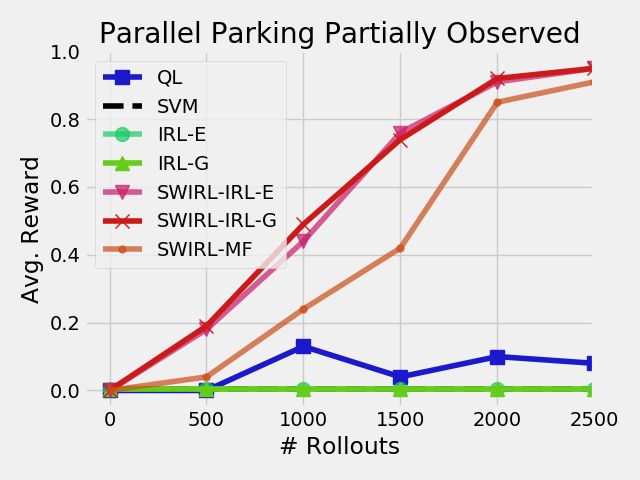
5

prior work (Krishnan* et al. 2015; Murali* et al. 2016), de-            Algorithm 1: Sequence Learning
scribes a number of practical optimizations such as pruning              Data: Demonstration D
low-confidence mixture components.                                  1    Fit a DP-GMM model to D and identify the set of transitions
   For each mixture component, we can define ellipsoids                   Θ, defined as all (xt ,t) where (xt+1 ,t + 1) has a different
by taking the confidence level-sets in the state-space and                cluster.
time that characterize regions where transitions occur.             2    Fit a DP-GMM to the states in Θ.
These regions are ordered since they are also defined over          3    Prune clusters that do not have one transition from all
                                                                          demonstrations.
time, since we make the assumption that the confidence
                                                                    4    The result of is G = [ρ1 , ρ2 , ..., ρm ] where each ρ is a disjoint
threshold for the level sets is tuned so that the regions                 ellipsoidal region of the state-space and time interval.
are disjoint. Thus, reaching one of these regions defines                Result: G
a testable condition based on the current state, time, and
previously reached regions–which is a Markov Segmentation
Function. The result is exactly the set of transition regions:      et al. 1998). By changing the kernel function (i.e., the
G = [ρ1 , ρ2 , ..., ρk ], and segmentation of each demonstration    similarity metric between states), we can essentially change
trajectory into k segments.                                         the definition of local linearity.
   In typical GMM formulations, one must specify the                   Let κ(xi , x j ) define a kernel function over the states.
number of mixture components k before hand. However, we             For example, if κ is the radial basis function (RBF),
apply results from Bayesian non-parametric statistics and                                    −kxi −x j k2
                                                                                                        2
jointly solve for the component parameters and the number           then: κ(xi , x j ) = e 2σ . κ naturally defines a matrix M
of components using a Dirichlet Process (Kulis and Jordan           where: Mi j = κ(xi , x j ). The top p0 eigenvalues define a new
                                                                                                                    0
2011). The DP places a soft-prior on the number of clusters.        embedded feature vector for each ω in R p . We can now
During inference, the number of components grows with               apply the algorithm above in this embedded feature space.
the complexity of the observed data (we denote this as DP-
GMM). The DP has hyper-parameters which we tune once
for all domains, we use a uniform base measure and a prior          5      Phase 2: Reward Learning
weight of 0.1.                                                      After the sequence learning phase, each demonstration is
                                                                    partitioned into k segments. The reward learning phase
4.3      GMM-based Segmentation                                     uses the learned [ρ1 , ..., ρk ] to construct the local rewards
As an instance of the general framework, we use                     [R1 , ..., Rk ] for the task. Each Ri is a quadratic cost
Gaussian Mixture Models to segment demonstrations in our            parametrized by a positive semi-definite matrix Q. The
experiments. This technique is quite general and applies to a       Algorithm is summarized in below in Phase 2.
large class of linear and non-linear systems.
   A popular approach for transition identification is to use       5.1       Primer on Maximum Entropy Inverse
Gaussian Mixture Models (Calinon 2014), namely, cluster                       Reinforcement Learning
all state observations and identify times at which xt is in a
different cluster than xt+1 . For a given time t, we can define     To fit the local rewards, we apply Maximum Entropy Inverse
a window of length ` as:                                            Reinforcement Learning (MaxEnt-IRL) (Ziebart et al. 2008).
                                                                    The goal of MaxEnt-IRL is to find a reward function such
                            (`)                                     that an optimal policy w.r.t that reward function is close to
                           nt = [xt−` , ..., xt ]|
                                                                    the expert demonstration. In the MaxEnt-IRL model, “close”
Then, for each demonstration trajectory we can also generate        is defined as matching the first moment of the expert feature
a trajectory of Ti − ` windowed states:                             distribution:
                                                                                                        N
                            (`)      (`)      (`)
                                                                                                   1 XX
                           di = [n` , ..., nTi ]                                         γexpert =         xi ,
                                                                                                   Z
                                                                                                            d∈D i=1
Over the entire set of windowed demonstrations, we collect a        where Z is an appropriate normalization constant (total
                        (`)
dataset of all of the nt vectors. We fit GMM model to these         number of states in all demonstrations). MaxEnt-IRL uses
vectors. The GMM model defines m multivariate Gaussian              the following linear parametrized representation:
                                                            (`)
distributions and a probability that each observation nt is
sampled from each of the m distributions. We annotate each                                           R(x) = xT θ ,
observation with the most likely mixture component. Times
            (`)      (`)
such that nt and nt+1 have different most likely components         where x is a feature vector representing the state of the
are marked as transitions. This has the interpretation of fitting   system. The agent is modeled as nosily optimal, where it
a locally linear regression to the data (refer to (Moldovan         takes actions from a policy π:
et al. 2015; Khansari-Zadeh and Billard 2011; Kruger et al.
2010; Krishnan* et al. 2015; Murali* et al. 2016) for details).                           π(a | s, θ ) ∝ exp{Aθ (s, a)}.
   If the system’s local dynamics are non-linear or
discontinuous, we can smooth out the dynamics with a                Aθ is the advantage function (Q function minus the Value
kernel embedding of the trajectories. The basic idea is             function) for the reward parameterized by θ . The objective
to apply Kernelized PCA to the features before learning             is to maximize the log-likelihood that the demonstration
the transitions–a technique used in Computer Vision (Mika           trajectories were generated by θ .

Prepared using sagej.cls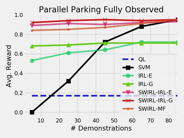
6                                                                                                                     Journal Title XX(X)

  Under the exponential distribution model, it can be shown             Algorithm 2: Reward Learning
that the gradient for this likelihood optimization is:                   Data: Demonstration D and sub-goals [ρ1 , ..., ρk ]
                           ∂L                                       1    Based on the transition states, segment each demonstration di
                              = γexpert − γθ ,                            into k sub-sequences where the jth is denoted by di [ j].
                           dθ
                                                                    2    Apply MaxEnt-IRL or Equation 1 to each set of sub-sequences
where γθ is the first moment of the feature distribution of an            1...k.
optimal policy under θ .                                                 Result: Rseq
   SWIRL applies MaxEnt-IRL to each segment of the task
but with a small modification to learn quadratic rewards
instead of linear ones. Let µi be the centroid of the next          applies MaxEnt-IRL to the sub-sequences of demonstrations
transition region. We want to learn a reward function of the        between 0 and ρ1 , and then from ρ1 to ρ2 and so on. The
form:                                                               result is an estimated local reward function Ri modeled as a
                Ri (x) = −(x − µi )T Q(x − µi ).                    linear function of states that is associated with each ρi .
for a positive semi-definite Q (negated since this is a negative    5.2.3 Model-free: Local Quadratic Rewards Sometimes
quadratic cost). With some re-parametrization (dropping µi          estimating the local dynamics can be unreliable if there
for convenience and without loss of generality), this reward        isn’t sufficient demonstration data. As a baseline, we also
function can be written as:                                         considered a much simpler reward learning approach that
                                  d X
                                  X d                               just estimates the covariance in each feature. Interestingly
                     Ri (x) = −             qi j x[ j]x[l].         enough, this approach worked reasonably well empirically
                                  j=1 l=1                           in many problems.
                                                                       The role of the reward function is to guide the robot to the
which is linear in the feature-space y = x[ j]x[l]:                 next transition region ρi . A straight forward thing approach
                               Ri (x) = θ T y.                      is for each segment i, we can define a reward function as
                                                                    follows:
5.2      Two Inference Settings: Discrete and                                            Ri (x) = −kx − µi k22 ,
         Continuous                                                 which is just the Euclidean distance to the centroid.
In MaxEnt-IRL gradient can be estimated reliably in two               A problem with using Euclidean distance directly is that it
cases, discrete and linear-gaussian systems, since it requires      uniformly penalizes disagreement with µ in all dimensions.
an efficient forward search of the policy given a particular        During different stages of a task, some features will likely
reward parametrized by θ . In both these cases, we have to          naturally vary more than others–this is learned through
estimate the system dynamics within each segment.                   IRL. To account for this, we derive a reasonable Q that is
                                                                    independent of the dynamics:
5.2.1    Discrete Consider the case when the state-space is
discrete (with cardinality N) and the action-space is discrete.                                Q[ j, l] = Σ−1
                                                                                                           x ,
To estimate the dynamics, we construct an N × N matrix
of zeros for each action and each of the components of              which is the inverse of the covariance matrix of all of the
this matrix corresponds to the transition probability of a          state vectors in the segment:
pair of states. For each, (s, a, s0 ) observation in the segment,                                        end
we increment (+1) the appropriate element of the matrix.
                                                                                                         X
                                                                                          Q[ j, l] = (         xxT )−1 ,              (1)
Finally, we normalize the elements to sum to one across the                                          t=start
set of actions. An additional optimization could be to add
smoothing to this estimate (i.e., initialize the matrix with        which is a p × p matrix defined as the covariance of all of
some non-zero constant value), we found that this was not           the states in the segment i − 1 to i. Intuitively, if a feature has
necessary on the sparse domains in our experiments. The             low variance during this segment, deviation in that feature
result is an estimate for the P(s0 | s, a). Given this estimate,    from the desired target it gets penalized. This is exactly the
γθ can be efficiently calculated with the forward-backward          Mahalonabis distance to the next transition.
technique described in (Ziebart et al. 2008).                          For example, suppose one of the features j measures the
                                                                    distance to a reference trajectory ut . Further, suppose in
5.2.2  Linear The discrete model is difficult to scale to           step one of the task the demonstrator’s actions are perfectly
continuous state-spaces. If we discretize, the number of            correlated with the trajectory (Qi [ j, j] is low where variance
bins required would be exponential in the dimensionality.           is in the distance) and in step two the actions are uncorrelated
However, linear models are another class of dynamics                with the reference trajectory (Qi [ j, j] is high). Thus, Q will
models for which the estimation and inference is tractable.         respectively penalize deviation from µi [ j] more in step one
We can fit local linear models to each of the segments              than in step two.
discovered in the previous section:
                               N seg
                               X   X j end
                                                    (i)       (i)
                                                                    6      Phase 3: Policy Learning
              A j = arg min                      kAxt − xt+1 k
                           A                                        SWIRL uses the learned transitions [ρ1 , ..., ρk ] and Rseq as
                               i=1 seg j start
                                                                    rewards for a Reinforcement Learning algorithm. In this
With A j known, γθ can be analytically solved with                  section, we describe learning a policy π given rewards Rseq
techniques proposed in (Ziebart et al. 2012). SWIRL                 and an ordered sequence of transitions G. However, this

Prepared using sagej.cls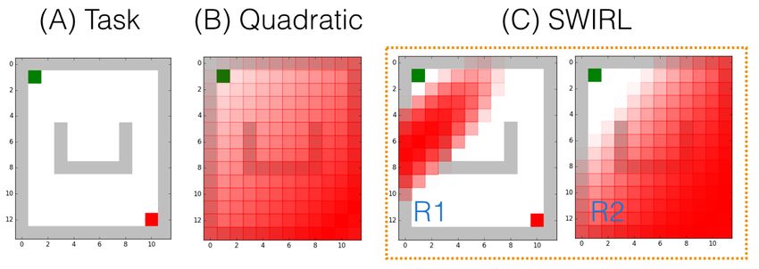
7

problem is not trivial since solving k independent problems         lifted space, the problem is a fully observed MDP. Then, the
neglects potential shared value structure between the local         additional complexity of representing the reward with history
problems (e.g., a common failure state). Furthermore,               over S × [k] is only O(k) instead of exponential in the time
simply taking the aggregate of the rewards can lead to              horizon.
inconsistencies since there is nothing enforcing the order
of operations. We show that a single policy can be learned          6.3    Segmented Q-Learning
jointly over all segments over a modified problem where the         At a high-level, the objective of standard Q-Learning is to
state-space with additional variables that keep track of the        learn the function Q(s, a) of the optimal policy, which is the
previously achieved segments.                                       expected reward the agent will receive taking action a in state
                                                                    s, assuming future behavior is optimal. Q-Learning works
6.1      Off Policy RL Algorithms                                   by first initializing a random Q function. Then, it samples
There are two classes of RL algorithms, on-policy algorithms        rollouts from an exploration policy collecting (s, a, r, s0 )
(e.g., Policy Gradients, Trust Region Policy Optimization)          tuples. From these tuples, one can calculate the following
and off-policy algorithms (e.g., Q-Learning). An on-policy          value:
algorithm learns the value of the policy being carried out by                         yi = R(s, a) + arg max Q(s0 , a)
                                                                                                           a
the agent and incrementally optimizes this policy. On policy
are often more efficient since the robot learns to optimize the     Each of the yi can be used to define a loss function since if
reward function in states that it is likely to visit, however,      Q were the true Q function, then the following recurrence
it requires that exploration is done with a specific policy         would hold:
that is continuously updated. On the other hand, off-policy
                                                                                  Q(s, a) = R(s, a) + arg max Q(s0 , a)
algorithms learn the value of the optimal policy regardless                                                    a
of the policy used to collect the data, as long the robot
                                                                    So, Q-Learning defines a loss:
sufficiently explores the space. This is highly beneficial for
our problem setting. A single fixed exploration policy can be                               X
                                                                                   L(Q) =       kyi − Q(s, a)k22
used to collect a large batch of data up front, which we can
                                                                                                  i
use to refine our model. This is the motivation for using a
Q-Learning approach in SWIRL.                                       This loss can be optimized with gradient descent. When
                                                                    the state and action space is discrete, the representation
6.2      Segmentation Introduces Memory                             of the Q function is a table, and we get the familiar Q-
                                                                    Learning algorithm–where each gradient step updates the
In our sequential task definition, we cannot transition to
                                                                    table with the appropriate value. When Q function needs
reward Ri+1 unless all previous transition regions ρ1 , ...ρi are
                                                                    to be approximated, then we get the Deep Q Network
reached in sequence. This introduces a dependence on the
                                                                    algorithm.
history which violates the MDP structure.
                                                                       SWIRL applies a variant of Q-Learning to optimize the
   Naively addressing this problem can lead to an exponential
                                                                    policy over the sequential rewards. This is summarized
cost in the state-representation. Given a finite-horizon MDP
                                                                    in Algorithm 3. The basic change to the algorithm is to
M as defined in Section 3, we can define an MDP MH
                                                                    augment the state-space with indicator vector that indicates
as follows. Let H denote set of all dynamically feasible
                                                                    the transition regions that have been reached. So each of the
sequences of length smaller than T comprised of the
                                                                    rollouts, now records a tuple (s, v, a, r, s0 , v’) that additionally
elements of S. Therefore, for an agent at any time t, there
                                                                    stores this information. The Q function is now defined over
is a sequence of previously visited states Ht ∈ H. The MDP
                                                                    states, actions, and segment index–which also selects the
MH is defined as:
                                                                    appropriate local reward function:
                MH = hS × H, A, P0 (·, ·), R(·, ·), T i.
                                                                               Q(s, a, v) = Rv (s, a) + arg max Q(s0 , a, v0 )
                                                                                                               a
For this MDP,        P0
                     not only defines the transitions from the
current state s 7→ s0 , but also increments the history sequence    We also need to define an exploration policy, i.e., a stochastic
Ht+1 = Ht ts. Accordingly, the parametrized reward function         policy with which we will collect rollouts. To initialize the
R is defined over S, A, and Ht+1 . MH allows us to address          Q-Learning, we apply Behavioral Cloning locally for each
the sequentiality problem since the reward is a function of         of the segments to get a policy πi . We apply an ε-greedy
the state and the history sequence. However, without some           version of these policies to collect rollouts.
parametrization of Ht , directly solving this MDPs with RL is       Remarks: Initializing with a Behavioral Cloning policy
impractical since it adds an overhead of O(eT ) states.             is not strictly necessary, and a random initialization would
   We can leverage the definition of the Markov Segmen-             suffice. In practice, we found that this was much more
tation function formalized earlier to avoid this exponential        efficient on problems where the difference between the
complexity. We know that the reward transitions (Ri to Ri+1 )       demonstration domain and execution domain was small.
only depend on an arrival at the transition state ρi and not
any other aspect of the history. Therefore, we can store an
index v, that indicates whether a transition state i ∈ 0, ..., k    7     Experiments
has been reached. This index can be efficiently incremented         We evaluate SWIRL on two standard RL benchmarks and in
when the current state s ∈ ρi+1 . The result is an augmented       deformable cutting and tensioning on the da Vinci surgical
state-space vs to account for previous progress. In this            robot.

Prepared using sagej.cls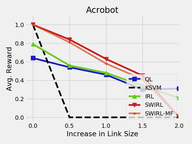
8                                                                                                              Journal Title XX(X)

     Algorithm 3: Policy Learning
      Data: Transition States G, Reward Sequence Rseq , exploration
              policy π
 1    Initialize Q( vs , a) randomly
 2    foreach iter ∈ 0, ..., I do
 3         Draw s0 from initial conditions
 4         Initialize v to be [0, ..., 0]
 5         Initialize j to be 1
 6         foreach t ∈ 0, ..., T do
 7              Choose best action a based on π.
 8              Observe Reward R j
 9              Update state to s0 and Q via Q-Learning update
10              If s0 is ∈ ρ j update v[ j] = 1 and j = j + 1
      Result: Policy π                                                Figure 3. For a fixed number of demonstrations 5, we vary the
                                                                      number of rollouts and measure the average reward at each
                                                                      rollout. (QL) denotes Q-learning, (SVM) denotes a baseline of
                                                                      behavioral cloning with a SVM policy representation, (IRL-E)
                                                                      denotes MaxEnt-IRL with estimated dynamics, (IRL-G) denotes
                                                                      MaxEnt-IRL with ground truth dynamics, (SWIRL-E) denotes
                                                                      SWIRL with local MaxEnt-IRL and estimated dynamics,
                                                                      (SWIRL-G) denotes SWIRL with local MaxEnt-IRL and ground
                                                                      truth dynamics, and (SWIRL-MF) denotes the model-free
                                                                      version of SWIRL. SWIRL achieves the same reward as QL with
                                                                      15% of the rollouts, and the same reward as IRL with 66% of
Figure 1. (A) Simulated control task with a car with noisy            the rollouts.
non-holonomic dynamics. The car (A1 ) is controlled by
accelerating and turning in discrete increments. The task is to
park the car between two obstacles.                                   hyperparameters k = 5, σ = 0.1 respectively. The radial basis
                                                                      function hyper-parameters were tuned manually to achieve
                                                                      the fastest convergence in the experimental task.
                                                                      Behavioral Cloning (SVM): We generated N demonstra-
                                                                      tions using an RRT motion planner (assuming deterministic
                                                                      dynamics). The next baseline is to directly learn a policy
                                                                      from the generated plans using behavioral cloning. We use
                                                                      an L1 hinge-loss SVM with L2 regularization α = 5e − 3
Figure 2. (Left) the 5 demonstration trajectories for the parallel
parking task, and (Right) the sub-goals learned by SWIRL.
                                                                      to predict the action from the state. The hyper-parameters
There are two intermediate goals corresponding to positioning         were tuned manually using cross-validation by holding out
the car and orienting the car correctly before reversing.             trajectories.
                                                                      Single-Step IRL (MaxEnt-IRL): We generated N demon-
                                                                      strations using an RRT motion planner (assuming determin-
7.1       Fully Observed Parallel Parking                             istic dynamics). We use the collected demonstrations and
We constructed a parallel parking scenario for a robot car            infer a quadratic reward function using MaxEnt-IRL (both
with non-holonomic dynamics and two obstacles (Figure 1a).            using estimated dynamics and ground truth dynamics). The
The car can accelerate or decelerate in discrete ±0.1 meters          learned reward function is optimized using Q-learning with
per second increments (the car can reverse), and change its           a radial basis function representation with the same hyper-
heading by 5◦ degree increments. The car’s speed (kẋk+kẏk)          parameters as the RL approach.
and heading (θ ) are inputs to a bicycle steering model which         SWIRL: Finally, we apply SWIRL to the N demonstrations,
computes the next state. The car observes its x position, y           learn segmentation, and quadratic rewards (Figure 2). We
position, orientation, and speed in a global coordinate frame.        apply SWIRL with a DP-GMM based segmentation step
The car’s dynamics are noisy and with probability 0.1 will            with no kernel transformation (as described in Section
randomly add or subtract 2.5◦ degrees to the steering angle.          4.3). For the local IRL approach, we consider three
If the car parks between the obstacles, i.e., 0 speed within          approaches: MaxEnt with ground truth dynamics, MaxEnt
a 15◦ tolerance and a positional tolerance of 5 meters, the           with locally estimated dynamics, Model-Free. The learned
task is a success and the car receives a reward of 1. If the          reward functions and transition regions are used in the policy
car collides with one of the obstacles or does not park in 200        learning phase with Q-learning with a radial basis function
timesteps, the episode ends with a reward of 0.                       representation with the same hyper-parameters as the RL
   We call this domain Parallel Parking with Full Observation         approach.
(PP-FO). We consider the following approaches:
RL (Q-Learning): The baseline approach is modeling the                7.1.1   Fixed Demonstrations, Varying Rollouts In the first
entire problem as an MDP with the sparse delayed reward.              experiment, we fix the number of initial demonstrations
We apply Q-Learning to learn a policy for this problem with           N = 5, and vary the number of rollouts (Figure 3). The
a radial basis function representation for the Q-function with        baseline line Q-Learning approach (QL) is very slow because

Prepared using sagej.cls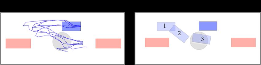
9

it relies on random exploration to achieve the goal at least
once before it can start estimating the value of states and
actions. However, given enough exploration (1250 rollouts),
Q-Learning converges to a solution with a 95% success rate.
In this problem, there will always be some failure cases
to the noise in the system. We collect five demonstrations
and directly learn a policy with an SVM. This policy has
a very poor success rate of 13%. Q-Learning and the SVM
define two extremes, no demonstrations, and no rollouts,
respectively.
   Next, we consider combinations of rollouts and demon-
strations. We apply MaxEnt-IRL to the five demonstrations
and learn reward functions. Since the MaxEnt-IRL inference
                                                                Figure 4. For 500 rollouts, we vary the number of
procedure requires a dynamics model, we consider two
                                                                demonstration trajectories given to each technique. (QL)
variants: (1) estimate the dynamics from the demonstrations,    denotes Q-learning, (SVM) denotes a baseline of behavioral
and (2) use the known dynamics model of the car directly.       cloning with a SVM policy representation, (IRL-E) denotes
We found that both IRL methods surpassed the SVM policy         MaxEnt-IRL with estimated dynamics, (IRL-G) denotes
after only 250 rollouts, and attained the same final reward     MaxEnt-IRL with ground truth dynamics, (SWIRL-E) denotes
as Q-Learning in 250 fewer rollouts. Surprisingly, we found     SWIRL with local MaxEnt-IRL and estimated dynamics,
that there was little difference between using the estimated    (SWIRL-G) denotes SWIRL with local MaxEnt-IRL and ground
                                                                truth dynamics, and (SWIRL-MF) denotes the model-free
dynamics model and the ground truth model.
                                                                version of SWIRL. SWIRL is less sensitive to the number of
   Finally, we considered three variants of SWIRL. (SWIRL-      demonstrations observed than the SVM. With only 5
E) is SWIRL with local MaxEnt-IRL and estimated                 demonstrations, SWIRL is within 10% of its reward if it observed
dynamics, (SWIRL-G) is SWIRL with local MaxEnt-IRL              100 demonstrations.
and ground truth dynamics, and (SWIRL-MF) denotes the
model-free version of SWIRL. SWIRL achieves the same
reward as QL with 15% of the rollouts, and the same
reward as IRL with 66% of the rollouts. SWIRL learns
three segments for this task (Figure 2), and places quadratic
rewards that guide the car to each of these segments. There
are two intermediate goals corresponding to positioning the
car and orienting the car correctly before reversing. With a
single quadratic reward (as in IRL), the car has to learn to
make a sequence of actions that move away from the goal
(pulling up). In the segmented problem, the car can always
move monotonically towards each of the goals.

7.1.2   Fixed Rollouts, Varying Demonstrations Next, we
fix the number of rollouts to 500 and vary the number           Figure 5. For 500 rollouts and 100 demonstrations, we
of demonstration trajectories each approach observes.           measure the robustness of the approaches to changes in the
The baseline line Q-Learning approach (QL) takes no             execution dynamics. (QL) denotes Q-learning, (SVM) denotes a
                                                                baseline of behavioral cloning with a SVM policy representation,
demonstrations and has a success rate of 17% after 500
                                                                (IRL-E) denotes MaxEnt-IRL with estimated dynamics, (IRL-G)
rollouts. The behavioral cloning approach (SVM) is sensitive    denotes MaxEnt-IRL with ground truth dynamics, (SL-E)
to the number of demonstrations it observes. For five           denotes SWIRL with local MaxEnt-IRL and estimated dynamics,
demonstrations, it achieves a success rate of only 13%. But     (SL-G) denotes SWIRL with local MaxEnt-IRL and ground truth
if it observes 100 demonstrations it can achieve nearly the     dynamics, and (SL-MF) denotes the model-free version of
maximum 95% success rate.                                       SWIRL. While the SVM is 95% successful on the original
                                                                domain, its success does not transfer to the perturbed setting.
   On the other hand, the IRL approaches and SWIRL are
                                                                On the other hand, SWIRL learns rewards and segments that
comparatively less sensitive–where they perform nearly as       transfer to the new dynamics since they are state-space goals.
well with a small number of demonstrations as they do with
a larger data set. With only five demonstrations, SWIRL is
within 10% of its reward if it observed 100 demonstrations.     demonstrations and learn to refine the initial policy through
In this task, the policy is more complex than the reward        exploration.
function, which is just a quadratic. It potentially requires
much less data to estimate a quadratic function.                7.1.3   Varying Task Parameters We also explored how
   The SVM approach does have the advantage that it doesn’t     well the approaches handle transfer if the dynamics
require any further exploration. However, SWIRL and the         change between demonstration and execution. We collect
SVM approach are not mutually exclusive. As we show in          demonstrations N = 100 on the original task, and then used
our physical experiments, we can initialize Q-learning with     the learned rewards or policies on a perturbed task. In the
a behavioral cloning policy. The combination of the two         perturbed task, the system dynamics are coupled in a way
approaches allows us to take advantage of a small number of     that turning right causes the car to accelerate forward by 0.05

Prepared using sagej.cls
10 Journal Title XX(X)
(x, y, θ ). As before, if the car collides with one of the obstacle
or does not park in 200 timesteps the episode ends. We call
this domain Parallel Parking with Partial Observation (PP-
PO).
This form of partial observation creates an interesting
challenge. There is no longer a stationary policy that can
achieve the reward. During the reversing phase of parallel
parking, the car does not know that it is currently reversing.
So there is ambiguity in that state whether to pull up or
reverse. We will see that segmentation can help disambiguate
the action in this state.
As before, we generated 5 demonstrations using an
RRT motion planner (assuming deterministic dynamics) and
Figure 6. We hid the velocity state from the robot, so the robot
applied each of the approaches. The techniques that model
only sees (x, y, θ ). For a fixed number of demonstrations 5, we
vary the number of rollouts and measure the average reward at this problem with a single MDP all fail to converge. The
each rollout. (QL) denotes Q-learning, (SVM) denotes a Q-Learning approach achieves some non-zero rewards by
baseline of behavioral cloning with a SVM policy representation, chance. The learned segments in SWIRL help disambiguate
(IRL-E) denotes MaxEnt-IRL with estimated dynamics, (IRL-G) dependence on history, since the segment indicator tells the
denotes MaxEnt-IRL with ground truth dynamics, (SWIRL-E) car which stage of the task is currently active (pulling up or
denotes SWIRL with local MaxEnt-IRL and estimated dynamics, reversing) After 250000 time-steps, the policy learned with
(SWIRL-G) denotes SWIRL with local MaxEnt-IRL and ground
model-based SWIRL has a 95% success rate in comparison
truth dynamics, and (SWIRL-MF) denotes the model-free
version of SWIRL. SWIRL converges will the other approaches to a11
Figure 7. We plot the centroids of the learned segments in SWIRL to visualize how SWIRL is partitioning the task. Qualitatively,
SWIRL constructs evenly-spaced way points along the swing up trajectory.
Figure 8. For a fixed number of demonstrations 5, we vary the Figure 9. For a number of rollouts 3000, we vary the number of
number of rollouts and measure the average reward at each demonstration trajectories given to each technique. QL)
rollout. (QL) denotes Q-learning, (KSVM) denotes a baseline of denotes Q-learning, (KSVM) denotes a baseline of behavioral
behavioral cloning with a Kernel SVM policy representation, cloning with a Kernel SVM policy representation, (IRL) denotes
(IRL) denotes MaxEnt-IRL using linearized dynamics learned MaxEnt-IRL using linearized dynamics learned from the
from the demonstrations, (SWIRL) denotes SWIRL with local demonstrations, (SWIRL) denotes SWIRL with local
MaxEnt-IRL and estimated linear dynamics, and (SWIRL-MF) MaxEnt-IRL and estimated linear dynamics, and (SWIRL-MF)
denotes the model-free version of SWIRL. SWIRL converges denotes the model-free version of SWIRL. SWIRL is less
with 2000 fewer rollouts than Q-learning and IRL. senstive to the number of demonstrations observed than the
SVM. With only 15 demonstrations, SWIRL is able to achieve
the maximum reward. In comparison, the SVM requires 250
α = 5e − 3 to predict the action from the state. The hyper- demonstrations.
parameters were tuned manually using cross-validation by
holding out trajectories.
significantly faster than Q-Learning. This is because it mod-
Single-Step IRL (MaxEnt-IRL): We generated N els the reward function as a single quadratic, but there are
demonstrations using the Q-Learning baseline (i.e., run to multiple steps required to swing the pendulum up. The single
convergence and sample from the learned policy). We use quadratic potentially misleads learner in early episodes.
the collected demonstrations and infer a quadratic reward Finally, we see that SWIRL converges with 2000 fewer
function using MaxEnt-IRL. In the acrobot, we only use rollouts than Q-learning and IRL. The model-free method
estimated dynamics because the underlying system is non- converges with 1000 more rollouts. This experiment suggests
linear. The estimated dynamics are a linearization. The that SWIRL is applicable to certain types of non-linear
learned reward function is optimized using Q-learning with systems. We defer a more formal study of this problem to
a radial basis function representation with the same hyper- future work.
parameters as the RL approach.
SWIRL: Finally, we apply SWIRL to the N demonstrations, 7.2.2 Varying Demonstrations, Fixed Rollouts Next, we
learn segmentation, and quadratic rewards (Figure 2). We fix the number of rollouts to 3000, and vary the number of
apply SWIRL with a DP-GMM based segmentation step demonstration trajectories each approach observes (Figure
with a kernel transformation σ = 0.1 (as described in 9). This task is substantially harder to learn than the
Section 4.3). For the local IRL approach, we consider parallel parking task. More demonstration data is required
two approaches: MaxEnt with locally estimated dynamics, to learn the segments, rewards, and policies. The basline
Model-Free. The learned reward functions and transition line Q-Learning approach (QL) takes no demonstrations
regions are used in the policy learning phase with Q-learning and has a success rate of 58% after 3000 rollouts. As
with a radial basis function representation with the same before, the behavioral cloning approach (KSVM) is sensitive
hyper-parameters as the RL approach. to the number of demonstrations it observes. For 50
demonstrations, it acheives a success rate of 0%. It requires
7.2.1 Fixed Demonstrations, Varying Rollouts We gen- 250 demonstrations to have a 100% success rate. Again,
erated N = 15 demonstrations for the Acrobot task and the IRL approaches and SWIRL are less sensitive–where
compared the different approaches (Figure 8). The baseline they perform nearly as well with a small number of
behavioral cloning policy with a kernel svm failed to suc- demonstrations as they do with a larger dataset. With only
ceed. Q-learning required 5000 rollouts to acheive a policy 15 demonstrations, SWIRL is able to achieve the maximum
that was successful 100% of the time. IRL did not converge reward.
Prepared using sagej.cls12 Journal Title XX(X)
7.3 Physical Experiments with the da Vinci
Surgical Robot
In the next set of experiments, we evaluate SWIRL on
two tasks on the da Vinci Surgical Robot. The da Vinci
Research Kit is a surgical robot originally designed for tele-
operation, and we consider autonomous execution of surgical
subtasks. Based on a chessboard calibration, we found that
the robot has an RMSE kinematic error of 3.5 mm, and thus,
requires feedback from vision for accurate manipulation. In
our robotic setup, there is an overhead endoscopic stereo
camera that can be used to find visual features for learning,
and it is located 650mm above the workspace. This camera
Figure 10. For a number of rollouts 3000 and 250 is registered to the workspace with a RSME calibration error
demonstrations, we measure the transfer as a function of of 2.2 mm.
varying the link size. (QL) denotes Q-learning, (KSVM) denotes
a baseline of behavioral cloning with a Kernel SVM policy 7.3.1 Deformable Sheet Tensioning: In the first experi-
representation, (IRL) denotes MaxEnt-IRL using linearized ment, we consider the task of deformable sheet tensioning.
dynamics learned from the demonstrations, (SWIRL) denotes The experimental setup is pictured in Figure 11. A sheet
SWIRL with local MaxEnt-IRL and estimated linear dynamics, of surgical gauze is fixtured at the two far corners using a
and (SWIRL-MF) denotes the model-free version of SWIRL.
pair of clips. The unclipped part of the gauze is allowed to
The KSVM policy fails as soon the link size is changed. SWIRL
is robust until the change becomes very large. rest on soft silicone padding. The robot’s task is to reach
for the unclipped part, grasp it, lift the gauze, and tension
the sheet to be as planar as possible. An open-loop policy
typically fails on this task because it requires some feedback
of whether gauze is properly grasped, how the gauze has
deformed after grasping, and visual feedback of whether the
gauze is planar. The task is sequential as some grasps pick
up more or less of the material and the flattening procedure
has to be accordingly modified.
The state-space is the 6 DoF end-effector position of the
robot, the current load on the wrist of the robot, and a visual
feature measuring the flatness of the gauze. This is done by a
set of fiducial markers on the gauze which are segmented
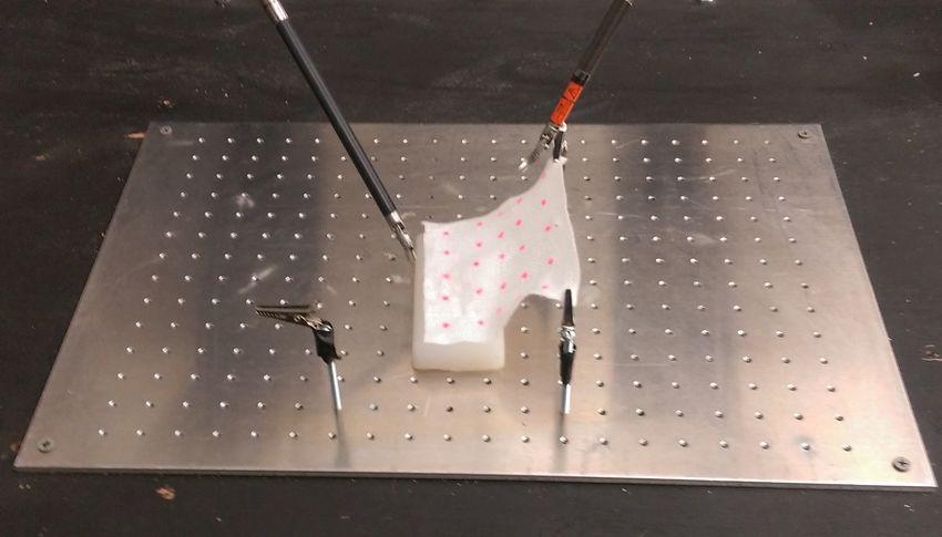
Figure 11. A sheet of surgical gauze is fixtured at the two far by color using the stereo camera. Then, we correspond
corners using a pair of clips. The unclipped part of the gauze is
the segmented contours and estimate a z position for each
allowed to rest on soft silicone padding. The robot’s task is to
reach for the unclipped part, grasp it, lift the gauze, and tension marker (relative to the horizontal plane). The variance in
the sheet to be as planar as possible. An open-loop policy the z position is a proxy for flatness and we include this
typically fails on this task because it requires some feedback of as a feature for learning (we call this disparity). The action
whether gauze is properly grasped, how the gauze has space is discretized into an 8 dimensional vector (±x, ±y,
deformed after grasping, and visual feedback of whether the ±z, open/close gripper) where the robot moves in 2mm
gauze is planar.The fiducial markers used to track the gauze are increments.
seen in red.
We provided 15 demonstrations through a keyboard-based
tele-operation interface. The average length of the demon-
strations was 48.4 actions (although we sampled observa-
7.2.3 Varying Task Parameters As in the parallel parking tions at a higher frequency about 10 observations for every
scenario, we evaluate how the different approaches handle action). From these 15 demonstrations, SWIRL identifies
transfer if the dynamics change between demonstration and four segments. Figure 12 illustrates the segmentation of a
execution. With N = 250 demonstrations, we learn the representative demonstration with important states plotted
rewards, policies, and segments on the standard pendulum, over time. One of the segments corresponds to moving to
and then during learning, we vary the size of the second link the correct grasping position, one corresponds to making the
in the pendulum. We plot the success rate (after a fixed 3000 grasp, one lifting the gauze up again, and one corresponds
rollouts) as a function of the increasing link size (Figure 10). to straightening the gauze. One of the interesting aspects of
As the link size increases the even the basline Q-learning this task is that the segmentation requires multiple features.
becomes less successful. This is because the system becomes Figure 12 plots three signals (current load, disparity, and
more unstable and it is harder to learn a policy. The z position), and segmenting any single signal may miss an
behavioral cloning SVM policy immediately fails as the link important feature.
size is increased. IRL is more robust but does not offer much Then, we tried to learn a policy from the rewards
of an advantage in this problem. SWIRL is robust until the constructed by SWIRL. In this experiment, we initialized
change in the link size becomes large. This is because for the the policy learning phase of SWIRL with the Behavioral
larger link size, SWIRL might require different segments (or Cloning policy. We define a Q-Network with a single-layer
one of the learned segments in unreachable). Multi-Layer Perceptron with 32 hidden units and sigmoid
Prepared using sagej.clsYou can also read