The Economic Burden of Pension Shortfalls: Evidence from House Prices

The Economic Burden of Pension Shortfalls:
 Evidence from House Prices∗
 Darren Aiello† Asaf Bernstein‡ Mahyar Kargar§ Ryan Lewis¶
 Michael Schwert∥

 October 26, 2021

 Abstract
 U.S. state pensions are underfunded by trillions of dollars, but their economic burden is un-
 clear. In a model of inefficient taxation, real estate fully reflects the cost of pension shortfalls
 when it is the only form of immobile capital. We study the effect of pension shortfalls on real
 estate values at state borders, where labor and physical capital could more easily relocate to
 a state with a smaller shortfall. Using plausibly exogenous variation driven by pension asset
 returns, we find that one dollar of pension underfunding reduces house prices near state bor-
 ders by approximately two dollars. Our estimates imply a deadweight loss associated with
 addressing pension shortfalls that is consistent with prior research in settings with high re-
 turns to public spending and costs of taxation.

 Keywords: Public finance, pensions, deadweight loss, real estate.
 JEL Classification: R3, H41, H55, H74.

 ∗ We thank Jeff Brown, Don Fullerton, Dan Garrett, Sean Myers, Taylor Nadauld, Robert Novy-Marx, Bill Schwert,
Qiping Xu, Jinyuan Zhang; and seminar participants at 2019 Financial Research Association (FRA) conference, Red
Rock Finance Conference 2021, SFS Cavalcade 2021, CU Boulder, Penn State, and UIUC for comments and sugges-
tions. We are very grateful to Lina Lu, Matt Pritsker, and Andrei Zlate for sharing their data on the sensitivity of
pension funds’ liabilities to interest rate changes. We also thank the UCLA Ziman Center’s Rosalinde and Arthur
Gilbert Program in Real Estate, Finance, and Urban Economics for their generous support. The first version of this
paper was circulated on November 4, 2019. All errors are our own responsibility.
 † Brigham Young University; d.a@byu.edu
 ‡ University of Colorado at Boulder - Leeds School of Business, and NBER; asaf.bernstein@colorado.edu
 § University of Illinois at Urbana-Champaign; kargar@illinois.edu
 ¶ University of Colorado at Boulder - Leeds School of Business; ryan.c.lewis@colorado.edu
 ∥ Corresponding Author; University of Pennsylvania; schwert@wharton.upenn.edu

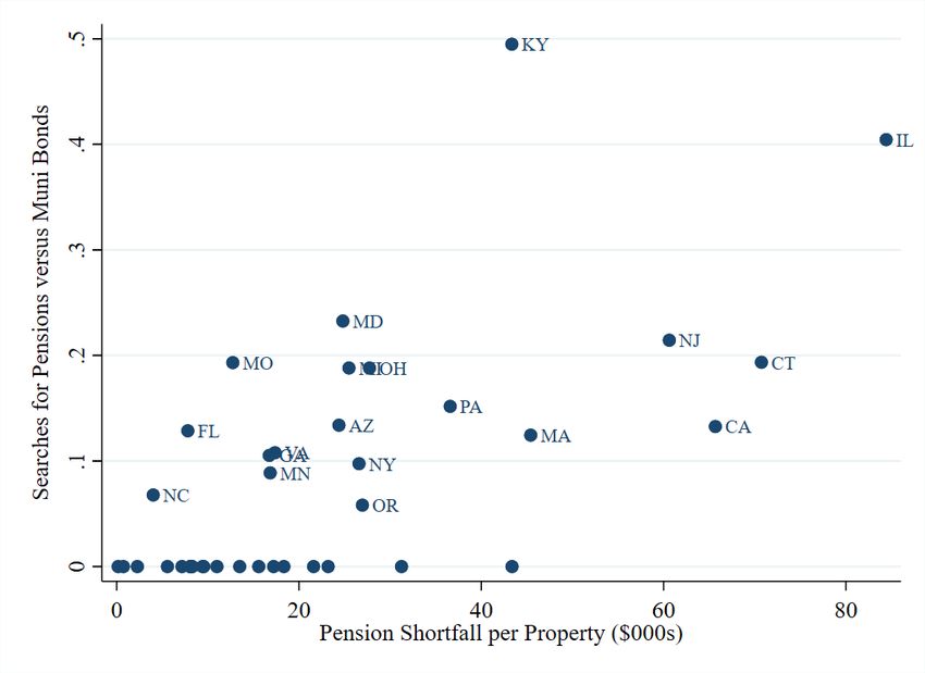
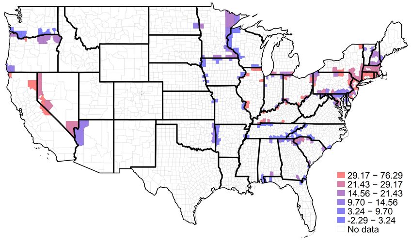
“Moody’s Investors Service estimates state and local pensions have unfunded liabilities of about $4
 trillion, roughly equal to the economy of Germany, the world’s fourth-largest economy.”
 — The Wall Street Journal, July 30, 20181

Underfunded public pensions in the U.S. represent an implicit household liability larger than
auto loans, student debt, and credit card balances combined.2 Despite popular concern about
pension shortfalls, little is known about the economic costs associated with addressing them.3
Several factors complicate the estimation of these costs, including the long maturity of pension
liabilities, the uncertain nature of pension asset returns, and the complex politics affecting the
size of pension promises and fund contributions.
 A model of inefficient taxation motivates our empirical strategy to identify the economic bur-
den of pension shortfalls. In an open economy, where capital and labor are mobile but real estate
is not, house prices reflect the total cost of pension shortfalls including any inefficiencies or dead-
weight loss generated in honoring the obligations (e.g., Oates, 1969; Bradford, 1978; Kotlikoff and
Summers, 1987; Harberger, 1995). Conversely, if all forms of capital face a high cost of relocation,
then the burden is unclear and the price on any individual asset is unlikely to reflect the true im-
plied cost. Motivated by this insight, we focus our analysis on locations near state borders where
immobile factors, such as real estate, should bear the burden and thus reflect the implied cost of
pension shortfalls. Since the level of pension underfunding may be affected by local economic
conditions and the endogenous response to past contributions and investment decisions, we use

 1 “The Pension Hole for U.S. Cities and States is the Size of Germany’s Economy”, available from: https://www.
wsj.com/articles/the-pension-hole-for-u-s-cities-and-states-is-the-size-of-japans-economy-1532972501.
 2 The state and local pension systems in the U.S. reported $1.378 trillion in unfunded liabilities in fiscal year 2015,
but according to Rauh (2016), who discounts cash flows using the Treasury curve to reflect the low risk of pension
promises, the accumulated deficit is $3.846 trillion. According to the Federal Reserve Bank of New York, as of the
fourth quarter of 2020, outstanding amounts of student loan, auto loan, and credit card debt are $1.55, $1.37, and
$0.82 trillion, respectively, totaling to $3.74 trillion.
 3 As evidence that the general public is interested in pension funding, Figure 1 shows a correlation of 0.65 between
state pension underfunding and state-level Google search intensity for “public pension” and “pension crisis.”

 1

plausibly exogenous variation in pension asset returns or “windfalls” to identify the causal effect
of pension shortfalls on house prices.
 Our main findings illustrate a consistent pattern: changes in pension funding pass through
to house prices in border counties and reflect a deadweight loss of addressing shortfalls. We es-
timate that the marginal home buyer is willing to pay approximately two dollars for each dollar
of additional pension funding per property. This house price pass-through is comparable to the
estimated impact of public spending on infrastructure and school salaries (e.g., Cellini, Ferreira,
and Rothstein, 2010; Bayer, Blair, and Whaley, 2020).4 Our theoretical framework shows that this
pass-through can be interpreted as a tax multiplier with respect to the funding of future liabilities
– for each additional dollar that states will have to raise through future taxes or amenity reduc-
tions, households perceive an economic burden of approximately two dollars. Controlling for
rental prices slightly decreases our pass-through estimates, which suggests that pension short-
falls affect house prices primarily through the capitalization of future costs and only partially
through the current quality of amenities.
 We face two major challenges in our empirical analysis. First, where businesses and indi-
viduals cannot easily avoid the future taxation associated with pension shortfalls, the burden of
taxes will be spread across all assets (i.e., human and physical capital as well as real estate). Thus,
we conduct our analysis at state borders, where businesses and individuals face a much lower
cost of relocating to a state with a smaller pension shortfall.5 This allows us to measure the eco-
nomic cost of pension shortfalls in areas where landowners are expected to bear the brunt of any
changes to taxes and the provision of government services.
 4 These estimates reflect spending on potentially “high value” projects. In this paper we study windfalls, so the
estimated pass-through reflects the marginal value of the best unfunded projects or the total burden of taxation.
 5 According to Rauh (2016), state pension plans account for $4.05 trillion (84%) of the $4.80 trillion total reported
pension liability, so our analysis captures most of the U.S. public pension burden. City and county borders would
also be natural settings if not for a lack of data on local government pensions, except for the largest municipalities,
that precludes our empirical strategy.

 2

This focus on state borders is one of the key features that distinguishes our paper from earlier
studies on the relation between pension funding and house prices in individual cities or states
(e.g., Epple and Schipper, 1981; Leeds, 1985; Hur, 2008; Albrecht, 2012; MacKay, 2014; Stadelmann
and Eichenberger, 2014). These studies do not focus on border areas where real estate is the only
immobile asset, so their estimates do not reflect the full economic cost of pension shortfalls. Thus,
we answer a fundamentally different question from these earlier papers, using housing markets
as a laboratory to measure an economic primitive rather than as the outcome of interest.6
 Second, pension underfunding is likely to be correlated with omitted variables. If shortfalls
were accrued in efforts to improve amenities for state residents, then states with high shortfalls
would provide better services than states with low shortfalls. Alternatively, if generous pensions
are the result of overinvestment in poorly performing projects, shortfalls may be associated with
worse quality of life. Our question requires exogenous variation to identify the causal effect of
shortfalls, so we focus on the effect of pension asset returns on house prices. We refine this
approach to account for potential “home bias” or “familiarity bias” in pension investments by
restricting attention to benchmark returns or unexpected excess returns over these benchmarks.
 In our baseline analysis, we compare the pension asset returns in the early part of our sample
(2002–2014) with home prices thereafter for properties in county clusters across state borders.
We find that increases in raw returns, excess returns, and benchmark returns implied by asset
allocations are all associated with increased house prices. To quantify the effect of pension short-
falls, we calculate cumulative dollar pension returns based on 2001 pension assets and find a
pass-through of approximately two – for each dollar of pension asset returns, house prices in-
crease by approximately two dollars. Nonparametric analysis of the border discontinuity reveals

 6 In fact, in an analysis of properties in the interior of the state, we find disperse and inconsistent estimates,
which is exactly what we would expect. In such settings the relative burden should be split among various forms of
capital in a way that depends on their relative mobility and elasticities and is likely to vary across regions.

 3

a clear increase in prices when moving from a low-return state to a high-return state.
 Our estimates are robust to a battery of alternative specifications. First, we consider asset
returns between 2002 and a property’s sale year, instead of using the same return horizon for
all houses, and find a similar pass-through of approximately two. The benefit of this approach
is that it allows us to include property fixed effects among properties with repeat sales. This
alleviates the concern that our findings could be driven by time-invariant factors at the state,
local, or property level. Focusing on the sub-sample of repeat sales provides a slightly lower
pass-through estimate. This is not surprising as requiring repeat sales on a property moves the
average transaction date forward in time, leaving less time on average between 2002 and the sale.
Prior work has shown it can take several years for even things like public spending on schools
to be fully realized in house prices (e.g., Bayer, Blair, and Whaley, 2020). More importantly, the
inclusion of property fixed effects has little effect on the overall pass-through in the repeat sales
sample, which suggests that unobservable time-invariant factors are not biasing our estimates.
 In supporting our focus on windfalls from pension returns instead of the level of pension
shortfalls, we provide novel evidence that pension investment returns “crowd out” pension fund
contributions. Specifically, we show that each dollar of excess pension returns is associated with
a 55 cent reduction in contributions. To our knowledge, we are the first to document this mecha-
nism in the academic literature. This finding highlights both the benefits of our empirical strategy,
which would be biased by a focus on the level of shortfalls, as well as the political incentives that
are likely responsible for the pension underfunding crisis.
 To shed light on the economic channels driving our results, we turn our attention to the
quality of government amenities and find that higher state-level pension shortfalls correlate with
less educational spending and poorer road quality. This raises a question: do our estimates reflect
worse current amenities in places with low pension asset returns, or an expectation of future costs

 4

that are capitalized in housing prices? To address this, we add time-varying local rental prices to
the set of control variables and find slightly attenuated results when measuring windfalls over
the entire sample period. While reaffirming that our results are not endogenously related to
economic conditions, this test also narrows the interpretation of our pass-through estimates: the
economic burden of pension shortfalls primarily reflects expectations about future increases in
taxes or decreases in the quality of amenities.7 Finally, we show that the estimated economic
burden is significantly higher in states that currently have higher income tax rates, consistent
with these states facing larger distortions associated with increasing tax rates to fund pension
obligations in the future.
 This paper contributes to the literature on the real effects of public finance. An emerging seg-
ment of this literature focuses on the condition of state and local pensions in the United States.
Earlier work in this area has focused on the measurement of the pension underfunding (Brown
and Wilcox, 2009; Novy-Marx and Rauh, 2011; Novy-Marx and Rauh, 2014), the political econ-
omy of pension funding (Brinkman, Coen-Pirani, and Sieg, 2018; Myers, 2021), and the impact
of pension funding on municipal borrowing costs (Novy-Marx and Rauh, 2012; Boyer, 2020), the
precautionary savings of households (Zhang, 2021), and the economic recovery after the financial
crisis (Shoag, 2013). We complement this work by estimating the effect of pension shortfalls on
house prices near state borders to quantify the current economic impact of this future burden.
 Our theoretical model highlights the analogy between this paper and earlier studies of ineffi-
cient taxation. In equilibrium, the effect of an exogenous increase in pension assets is equal to the
 7 An implication of this argument is that marginal home buyers are aware of the condition of local government
finances to the extent that they anticipate future tax hikes or reduced service provision. Since prices are based on
common signals such as comparable recent property transactions, this does not require that all households are aware
but only that marginal ones are. Although we cannot provide direct evidence on how households become informed
about pension underfunding, Google search trends (Figure 1) reveal that residents of states with worse pension
shortfalls are more interested in the issue. Underprovision of maintenance (e.g., poor roads) might signal information
about future conditions even though it provides little disamenity in the present. More directly, homeowners could
become informed from news coverage of state fiscal issues.

 5

present value of the tax multiplier, which means the pass-through of pension shortfalls to house
prices is comparable to other estimates of the economic burden of raising taxes. Consistent with
our estimates, Cellini, Ferreira, and Rothstein (2010) and Bayer, Blair, and Whaley (2020) find
economic costs between one and two dollars per dollar of tax revenue in the context of public
school spending.
 The empirical finding that unfunded pension liabilities are capitalized in house prices is in-
dicative of households’ forward-looking behavior. This evidence is also relevant to the applica-
bility of Ricardian equivalence (Barro, 1974). Although our goal is not to test whether Ricardian
equivalence holds, our findings are consistent with households internalizing the government’s
future budget constraint in their optimization problems.
 Finally, our results have implications for the political economy of public sector employee com-
pensation. Fitzpatrick (2015) estimates that public school employees in Illinois are willing to pay
20 cents on average for a one dollar increase in the present value of retirement benefits. We find
that households perceive substantial deadweight loss associated with addressing pension short-
falls. In combination, these findings question the efficiency of governments promising generous
retirement benefits to employees who do not value them and imposing the burden of funding
those promises on households who view them as costly.
 The remainder of the paper is organized as follows. Section 1 presents a model of tax burden
to motivate our empirical analysis. Section 2 describes our data on public pension funding and
house transaction prices. Section 3 explains our identification strategy. Section 4 presents the
main results. Section 5 concludes.

 6

1 Theoretical Framework

 In this section, we present a theoretical framework that motivates our research question and
identification strategy. We first show that in an open economy, landowners of a state within a
country are likely to bear the burden of a tax levied on a domestically mobile factor, motivating
our empirical design. We then show that the pass-through of pension shortfalls to house prices
is theoretically ambiguous and therefore an empirical question that reflects inefficiency in the
public provision of goods and capital raising.

1.1 Tax burden in an open economy

 Harberger (1962) argues that in a closed economy, the burden of the corporate income tax
tends to fall entirely on physical capital. Importantly, in a closed economy, untaxed factors al-
ways bear some burden of the tax if the taxed factor’s supply (demand) is not perfectly inelastic
(elastic).8 Relaxing the closed-economy assumption, most studies argue that in an open econ-
omy, immobile factors bear most, if not all, of the long-run burden of the tax in the economy
due to capital mobility across borders.9 Thus, it is critical for our empirical design to focus on an
open-economy setting at state borders to measure the burden of pension shortfalls.
 In Appendix A.2, we provide a simple framework based on Kotlikoff and Summers (1987)
to illustrate this point. There are two factors of production for the single good in the economy:
capital and land. Following Harberger (1962), we assume perfect competition and a fixed national
capital stock that is perfectly mobile within the country. For simplicity, we assume that the
factor complementary to capital, here labeled land, is supplied inelastically and is immobile. Since

 8 In Appendix A.1, we present a simple closed-economy framework to illustrate this point.
 9 Notableexamples include Bradford (1978), Kotlikoff and Summers (1987), Mutti and Grubert (1985), Harberger
(1995), and Gravelle and Smetters (2001). See Gravelle (2013) for a review of tax burden in general equilibrium.

 7

capital is mobile, rental rates on capital must be equalized across states: a tax imposed on income
earned by capital in a state is not fully borne by the capital initially located in the state imposing
the tax. In contrast, landowners in the two states are differentially impacted: there is a loss of
rental income in the state imposing the tax on capital and a gain in the other state. We summarize
the main takeaway of the open-economy model in Proposition 1.

Proposition 1. In an open economy, the immobile factor in a state is likely to bear a significant
portion of the burden of a tax that the state levies on a domestically mobile factor.

Proof. See Appendix A.4.

1.2 Pension shortfalls, tax distortions, and property values

 The previous section establishes that an open economy is the appropriate setting for our em-
pirical analysis. In this section, we study the capitalization of future pension liabilities in current
house prices. Whereas the previous section focused on capital mobility and the elasticity of de-
mand, this section introduces a role for asset prices. The economic burden of a tax is affected by
changes in asset prices due to the discounted present values of future tax and public expenditure
changes. We argue that the magnitude of the marginal decrease in house prices from an additional
dollar of pension shortfalls is theoretically ambiguous and therefore an empirical question.
 The model presented here is based on a slight modification of the asset-price approach to tax
burden presented in Poterba (1984). The key component of the burden is the price change for
existing owner-occupied homes due to the change in the present value of future taxes associated
with the asset. The stock of houses is assumed to be fixed in the short run, so the equilibrium
rental rate equates the demanded quantity with the existing housing services flow. Denote the
market-clearing rental rate by ( ) with ′ < 0, where is the inverse demand function for
housing services. ( ) represents the marginal benefit of housing services.

 8

Households consume housing services until the marginal value of these services equals their
marginal cost. We assume all houses incur depreciation at a constant rate per period, mainte-
nance costs equal to a fraction of the current value, and property taxes at a rate . All households
face a marginal income tax rate , can deduct property taxes from taxable income, and can bor-
row and lend at the nominal interest rate . The cost also includes any capital gain or loss of
holding the asset. Let , be the house price at the start of period , so ( , +1 − , ) represents
the capital gain or loss during period . In equilibrium, homeowners equalize the marginal cost
and marginal benefit of housing services:

 ( ) = , − ( , +1 − , ) , (1)

where ≡ + + (1 − )( + ).
 Consider a tax on each house that takes the form of a lump-sum payment to cover the
unfunded pension liability in period .10 We assume taxes induce a deadweight loss,

 = (1 + ) , (2)

where > 0. This means that to fund each additional dollar of pension liability in period , the
state has to raise more than one dollar in taxes. Parameter reflects the cost of raising revenues,
which we later estimate empirically.
 Because houses are durable assets, future taxes can still depress prices today. In each period
when the tax is levied, the equilibrium condition (1) becomes

 ( ) − = , − ( , +1 − , ) . (3)

 10 The tax payment is isomorphic to reducing current amenities to cover the liability .

 9

Since , +1 is unknown at time , we can solve the price , forward by rewriting (3) as

 ( ) − + , +1
 , = . (4)
 1+ 

Iterating Equation (4) forward and applying the no-bubble condition11 , the distortionary tax as-
sumption in (2) gives
 ∞ ∞
 ( + ) (1 + ) + 
 , = ∑ +1 − ∑ +1 . (5)
 =0 (1 + ) =0 (1 + )

The second term in Equation (5) is the present value of current and future tax payments to cover
pension liabilities. It is clear from (5) that if two states face the same housing demand curves but
have different levels of liabilities , all else equal, the one with a higher present value of pension
obligations will have lower house prices today.
 If the stock of housing is fixed12 (i.e., + = for all ), then from Equation (5) we can
determine the impact of an unfunded liability periods ahead on house prices today:

 , 1+ 
 =− < 0. (6)
 + (1 + ) +1

With reasonable parameter values for income and property tax rates, depreciation, and main-
tenance costs, the capitalization of future pension liabilities in house prices today can have a
magnitude of less or greater than one. It depends on how large the distortion is and how far in
the future the tax is imposed. We summarize the main message in Proposition 2.

 11 The transversality (no-bubble) condition in our setting is lim , + 
 →∞ (1+ ) +1 = 0, which rules out exploding house
prices. This condition is consistent with Giglio, Maggiori, and Stroebel (2016), who find no evidence of violations of
the transversality condition in the U.K. and Singapore housing markets, even during periods when housing bubbles
were thought to be present.
 12 With an endogenous housing stock, changes in future taxes induced by future pension liabilities will also affect
current and future investment in housing construction and the stock of housing { + }∞ =0 . In general, the effect of
housing stock adjustments can mitigate the effect of taxes on house prices. See Poterba (1984) for more details.

 10

Proposition 2. The magnitude of the marginal decrease in current house prices from an additional
dollar of pension shortfalls is ambiguous; it can be smaller or larger than one.

Proof. See Appendix A.4.

2 Data

2.1 State and local public pension plans database

 We obtain accounting and actuarial data for state and local pension plans from the Public
Plans Database (PPD) from the Center for Retirement Research at Boston College. PPD contains
annual plan-level data from 2001 through 2019 for 190 pension plans: 114 administered at the
state level and 76 administered locally. This sample covers 95% of public pension membership
and assets nationwide.13 The PPD is updated each spring from data available in the most recent
Comprehensive Annual Financial Reports (CAFRs) and Actuarial Valuations (AVs). Intermediate
updates may occur when new variables are added or data errors are corrected.
 We use the PPD data to calculate the plan-level pension shortfall defined as the actuarial ac-
crued liabilities less the market value of assets. Actuarial accrued liabilities, measured under tra-
ditional Governmental Accounting Standards Board (GASB) 25 standards, are equal to the present
value of future benefits, discounted using the plan’s assumed long-term investment return.

2.2 Detailed investment data by asset class

 The PPD includes detailed annual data on each plan’s specific asset allocations, returns by
asset class, and the associated benchmark returns. The asset classes in the PPD are based on the
 13 ThePPD sample is carried over from the Public Fund Survey (PFS), which was constructed with an emphasis
on the largest state-administered plans in each state, but also includes some large local plans such as New York City
ERS and Chicago Teachers. See https://publicplansdata.org/ for more details.

 11

categories reported by plans. We use these data to calculate the cumulative pension plan returns
used as instruments for pension shortfalls.14
 Table 1 reports descriptive statistics on the PPD data. On average across time and funds, the
largest asset holdings were equities and fixed income (53% and 28% of total assets, respectively),
followed by real estate and private equity (6% and 5% of total assets, respectively). The value of
assets is 79% of the actuarial value of liabilities for the mean observation, indicative of substantial
underfunding. Appendix Figure A.1 shows that the average ratio of pension assets to liabilities
declined from just above 100% in 2001 to 76.4% in 2019, reflecting an increase in underfunding
over the period we study.
 As discussed in Novy-Marx and Rauh (2011) and Rauh (2016), public pension liabilities are ef-
fectively risk-free, so the appropriate discount rate for valuing them is the yield on a zero-coupon
Treasury bond with the same duration. To discount pension liabilities using Treasury rates, we
need to calculate the duration and convexity of each plan. Unfortunately, the information neces-
sary for this calculation is unavailable in the PPD database prior to changes in pension reporting
standards in 2014.15 Therefore, to adjust the liability discount rate we use the aggregate adjust-
ment factor in Rauh (2016) and inflate unfunded liabilities by a constant factor of 2.86.16 While
we acknowledge this is an imperfect adjustment method, any resulting bias would affect only our
analysis of shortfalls and not the analysis that exploits variation in pension asset returns.

 14 The pension return data in the PPD have been used in academic research by Lu, Pritsker, Zlate, Anadu, and
Bohn (2019), among others.
 15 Under new GASB 67 guidelines, plans are required to disclose their total pension liabilities (TPL) under alter-
native scenarios of the discount rate being 100 bps higher (TPL +1% ) and 100 bps lower (TPL −1% ). However, this
information is only available starting in fiscal year 2014, when GASB 67 became effective.
 16 In fiscal year 2014, the state and local pension systems in the United States reported aggregate unfunded pension
liabilities of $1.19 trillion under GASB 67. Rauh (2016) applies a correction on a plan-by-plan basis that results in
aggregate unfunded accumulated benefits of $3.41 trillion under Treasury yield discounting. This implies an average
adjustment factor of 3.412/1.191 = 2.864.

 12

2.3 Zillow transaction and assessment database

 We obtain property-level data from the Zillow Transaction and Assessment Dataset (ZTRAX).
ZTRAX is, to the best of our knowledge, the largest national real estate database, with informa-
tion on more than 374 million detailed public records across 2,750 U.S. counties. It also includes
detailed assessor data including property characteristics, geographic information, and valuations
on over 200 million parcels in over 3,100 counties. These data have been used by Bernstein,
Gustafson, and Lewis (2019), among others.
 We filter the Zillow data in three ways. First we retain only residential property transactions
for which the price of the transaction is verified by the closing documents as being between the
typical home values in the the bottom and top market tiers as calculated at the county-month level
by the Zillow Home Value Index (ZHVI).17 Second, we focus only on single-family residences.
Third, in our primary empirical analysis we restrict attention to properties located in counties
sharing a border with an adjacent state and are located within 50 miles of the border.

3 Empirical Methodology

 The objective of this paper is to estimate the economic burden of temporally distant and un-
certain public liabilities. We focus on state pension shortfalls because of the growing concern
about their magnitude (Rauh, 2016). We examine the impact on real estate values near state bor-
ders because according to theory, they should reflect the perceived economic burden of shortfalls.
 First, property values provide a parsimonious and direct measure of the perceived present

 17 The ZHVI provides separate time series for the bottom market tier (33rd percentile and below of home values)
and for the top market tier (67th percentile and above of home values), representing typical home values in these
tiers. We impose an additional floor of $30,000 on the bottom tier and an additional ceiling of $2,000,000 on the top
tier to avoid data quality issues. Given that Zillow obtains prices from a variety of third-party sources and anecdotal
evidence suggests that these prices are occasionally incorrect, this filter improves the quality of our data.

 13

value of all future costs and benefits for homeowners. Unlike many assets, long-run discount
rates in housing tend to be quite low, increasing the plausibility that temporally distant costs
could significantly impact current prices (Giglio, Maggiori, and Stroebel, 2014). Also, for many
households their home is the largest financial investment, and prices are likely to reflect percep-
tions when the stakes are highest.
 Second, real estate is effectively immobile. As detailed in Section 1, property bears the full
brunt of inefficiencies in public capital raising in settings where other capital, consumers, and
labor can easily move, such as near state borders. While prior studies have looked at the cor-
relation between pension underfunding and house prices (e.g., Leeds, 1985; Hur, 2008; Albrecht,
2012; MacKay, 2014; Stadelmann and Eichenberger, 2014; Brinkman, Coen-Pirani, and Sieg, 2018),
none focus on border regions. We argue that this is critical for properly measuring the economic
burden of pension shortfalls. In addition, these earlier studies suffer from endogeneity in the
determinants of shortfalls, which preclude a causal interpretation.
 Therefore, we investigate how variation in net pension liabilities per capita, all else equal,
translates into variation in property values in regions near state borders. Consider the following
border discontinuity design (BDD) regression:

 = ℎ + + + + ′ + , (7)

where is the transaction price of house and ℎ 
is the estimated pension shortfall per property in state , in thousands of dollars, in year . 
are border county pairs interacted with time fixed effects that allow us to compare properties
transacting in physically adjacent regions, just across the state border from each other, in the
same time period. This approximates the empirical design suggested by our theoretical frame-

 14

work for an open economy. is the distance to the state border from the property’s centroid. If
the pension burden is reflected in property values, we would expect prices to jump suddenly at
the state border, when shortfalls also jump, even after the inclusion of this distance control. are
location fixed effects that capture time-invariant differences by region and region interacted with
property characteristics. These include zip code, zip code interacted with property characteris-
tics, and property fixed effects. Therefore, we obtain identification not only from cross-sectional
differences across state borders, but from variation in state pension funding status and house
prices over time in a border county relative to an adjacent county across the border. Finally, 
is a vector of time-varying continuous economic controls at the state-year or county-year level.
 Figure A.2 illustrates the counties involved in the discontinuity design along with the aver-
age shortfall throughout the sample. Our analysis requires sufficient population density to have
contemporaneous transactions on either side of the border among comparable property types.
 Our theoretical framework suggests that the BDD on shortfalls is an improvement over ex-
isting work because of its focus on border regions. However, we still face endogeneity concerns
similar to those present in the prior literature. Suppose a state chose to increase local spend-
ing on public services instead of funding its pension plans. These sorts of expenditures have
been shown to raise property values (e.g., Cellini, Ferreira, and Rothstein, 2010; Bayer, Blair, and
Whaley, 2020) and would mechanically increase net pension liabilities per capita. In this case,
the estimated pass-through between shortfalls and house prices would understate the economic
burden borne by households and could even have the wrong sign. Conversely, if shortfalls are
the result of poorly performing expenditures that have negative economic consequences for the
state, then the estimated burden may be biased upward.
 An ideal empirical setting supplies exogenous, as good as random, shocks to pension short-
falls that allow us to compare real estate transactions before and after the shocks. We therefore

 15

focus our analysis on pension asset returns, which cause immediate changes in unfunded pension
liabilities driven by factors that are plausibly exogenous to state expenditures. We implement the
same empirical design as Equation (7), substituting pension shortfalls with asset performance
“windfalls:”

 = + + + + ′ + , (8)

where is the compounded cumulative return for the pension
plans of state from the beginning of the sample (2002) to the transaction date or interim period
of interest (as explained in Section 4.1) multiplied by the assets per property in that state at the
beginning of the sample. This can be interpreted as the additional pension assets available per
property caused by performance of that state’s investment portfolio over that period. The regres-
sion coefficient represents the economic burden, which is equal to one plus the deadweight loss,
 , from our theoretical model in Equation (2). The economic interpretation is consistent with the
pass-through in our theoretical motivation because one dollar lower windfall per property implies
one dollar of additional pension shortfall per property.
 We also consider two-stage least squares (2SLS) designs that recover the economic burden of
pension underfunding while alleviating some remaining identification concerns. While our focus
on asset returns in border counties reduces many concerns about endogeneity, it is still possible
that pension funds’ home or familiarity biases (Hochberg and Rauh, 2013) could induce mechan-
ical relations between pension returns and local economic conditions. First, pension managers
may buy shares in local firms so that when the local economy does well, both the pension assets
and home prices appreciate (home bias). Second, pension managers may overallocate to indus-
tries or asset classes that are relatively abundant in a state, inducing a positive correlation between

 16

those industries, local economic conditions, and pension returns (familiarity bias). Conversely,
pension funds may be used to hedge a state’s fundamental risks, resulting in a negative correlation
between state economic activity and returns. For example, Texas-based managers with home bias
(hedging concerns) might overweight (underweight) both Texan firms and energy-related assets
generally.
 To alleviate these concerns, we estimate the following 2SLS regression:

 ̂
 = ′
 + + + + + ,

 = + + + + ′ + , (9)

where is an instrumental variable that exploits plausibly exogenous
variation in pension asset performance. First, we instrument for pension returns using returns in
excess of listed benchmarks, which mitigates the familiarity bias concern about the asset category
composition of the pension portfolio. However, this first approach leaves open the possibility
of home bias where outperformance of local firms drives excess pension returns and provides
spoils for the entire state. To alleviate concerns of home bias, we instrument for pension returns
using the returns of benchmark assets. To address both concerns simultaneously, we multiply
allocations to asset classes that have less potential to be localized (i.e., bonds and equities, and
funds that invest in them, rather than commodities, private debt, and real estate) by the relevant
benchmark returns from all pensions in the country.18 In this setup, returns should be unrelated
to both local economic conditions and state governance.

 18 Appendix Table A.1 details the asset classes reported in the PPD and delineates which are included in the
restricted benchmark return calculations.

 17

4 Results

4.1 Pension windfalls and property values near state borders

 In this section we exploit variation in pension funding coming from windfalls caused by the
realized performance of invested pension assets. Our analysis follows the baseline regression in
Equation (8), including border county group by year fixed effects that effectively compare the
property value at sale of houses in adjacent counties transacting in the same year but in states
with different pension windfalls. The group by time fixed effects absorb local trends in economic
activity. We control for income per capita at the state level to further alleviate concerns that
differential trends in economic activity across the state border affect our estimates. Lastly, we
include a continuous measure of distance to the border and a set of fixed effects that controls
flexibly for property characteristics.
 Within this framework, we begin by using cross-sectional variation in pension asset perfor-
mance over most of the sample period. In particular, we compare property transaction prices
from 2015 to 2018 occurring near state borders where one state had higher pension asset returns
from 2002 to 2014 than the other. We focus on this specification for two reasons. First, unless
homebuyers are perfectly rational and pay close attention to the evolution of pension funding
ratios, short-term variation in asset values is unlikely to impact home prices.19 Second, to the ex-
tent that observable degradation or improvement in public amenities operates as a signal about
the financial position of the state government, these effects would likely accumulate over long
periods of time.
 The pass-through of pension performance to house prices requires that home buyers have
some awareness of pension funding. However, it is only necessary that a subset of residents be
 19 Bayer,
 Blair, and Whaley (2020) find it can take several years for property values to reflect the underprovision
of educational public goods.

 18

aware of pension funding for it to have an impact on the housing market equilibrium. In support
of this prerequisite, Figure 1 presents Google Trends data showing that internet search volume
related to public pensions is higher in states with larger pension shortfalls. In particular, there
is a correlation of 0.65 between state level pension shortfalls per household and Google search
activity for “pension crisis” and “public pension”. States like Illinois, Kentucky, and New Jersey
have some of the worst-funded pensions and the most local interest in this issue. This suggests
that homeowners are likely aware of the financial problems plaguing their state governments,
especially in states with the largest shortfalls.
 Table 3 presents formal evidence of how such concerns are reflected in property values. We
estimate a BDD that compares house values in adjacent regions just across state borders with
varying levels of pension funding caused by pension asset performance from 2002 to 2014. We
construct the independent variable of interest as the product of the cumulative pension portfolio
return from 2002 to 2014 and the 2001 pension assets per property, which represents the dollar
windfall per property. Column (1) reports a positive and statistically significant coefficient of
2.42, which suggests a rise of about two dollars in property values for each dollar of additional
pension funding caused by state pension investment outperformance.
 Our theoretical framework shows that in a perfectly rational setting with otherwise equiv-
alent circumstances across borders, the coefficient on pension asset returns can be mapped di-
rectly to the cost of raising revenues in our model, denoted by . For instance, a coefficient of 2.42
suggests that the marginal cost of raising one dollar to pay back pension obligations is $2.42 of
total economic burden, including a deadweight loss of $1.42. As discussed in Section 1.2, a pass-
through larger than one is not surprising. In a related context, the effect of investment in public
education on house prices is also estimated to be large, implying a pass-through in our frame-
work of between one and two (Cellini, Ferreira, and Rothstein, 2010; Bayer, Blair, and Whaley,

 19

2020). In this light, our pass-through estimates are consistent with an underprovision of public
goods or services, perhaps driven by severe underfunding of pensions, which is relaxed by higher
returns on pension investments.

4.2 Addressing identification concerns

 This section examines potential biases in the estimate presented above. As noted previously,
the relative performance of pension assets still has the potential to be endogenously related to
state-level outcomes due to familiarity or home bias. We work to alleviate these concerns by re-
stricting variation in pension returns using an instrumental variables framework. An alternative
concern with the above approach is that it relies on a single measure of pension windfalls for
each state, which could be correlated with unobservable time-invariant state characteristics. We
address this concern by constructing a time-varying measure of pension returns and employing
property fixed effects. Finally, we present nonparametric estimates of the border discontinuity to
ensure the results are not an artifact of our linear regression specification.
 In the case of familiarity bias, invested asset composition could be driven by familiarity with
the sectors prevalent in a region (e.g., timber in Minnesota), inducing a correlation between pen-
sion returns and local economic outcomes. Column (2) of Table 3 includes the same sample and
control variables as column (1) but incorporates an instrumental variable for the pension windfall
in the 2SLS specification of Equation (9) using the initial assets per property in 2001 multiplied
by the cumulative pension fund performance from 2002–2014 in excess of the mean benchmark
performance for each asset class. This restricts variation to relative outperformance within each
asset class, rather than variation in allocation across asset classes or sectors. If familiarity bias
were driving our results, then using excess returns should eliminate any composition effect on
portfolio returns as long as the benchmarks are well specified. Column (2) reports a similar esti-

 20

mate for the economic burden (2.53) that is statistically significant with a strong first stage. This
suggests that familiarity bias is unlikely to drive our findings.
 However, this still leaves the possibility that home bias could be affecting our estimates. In
this case, even within an asset class a pension fund might be more likely to invest in local firms
(e.g., Minnesota equities in the Minnesota pension fund). To address this possibility, column (3)
takes the pension portfolio composition and applies the benchmark returns of each asset class to
calculate implied portfolio returns and reports a similar estimate of the economic burden (2.39).
To simultaneously shut down the familiarity channel, in column (4) we collapse the benchmarks
into major categories and omit niche asset classes to form our Restricted Benchmarks. Specifi-
cally, we restrict attention to assets that have less potential to be localized (i.e., bonds and equities,
and funds that invest in them, rather than commodities, private debt, and real estate). Again, we
find a similar estimate of the economic burden (2.39), suggesting little evidence of home bias in
our primary specification.
 One remaining concern with the evidence presented thus far is that it relies on purely cross-
sectional variation, so any time-invariant differences across state borders that correlate with pen-
sion asset performance could confound identification. To help alleviate this concern, we adjust
the independent variable of interest to be the cumulative return between 2002 and the transaction
date of the property. This specification allows us to control for unobservable time-invariant con-
founds, but has a downside relative to our baseline model. Since the sample includes transactions
with a shorter window over which pension returns are measured, the regression estimates could
be attenuated if it takes time for pension performance to be reflected in property values. This is
especially true when we require a house to have repeat sales, which mechanically tilts the sample
towards earlier observations.
 The first column of Table 4 replicates the regression in column (1) of Table 3 using the rolling

 21

measure of cumulative pension returns. This specification yields a positive and significant coeffi-
cient of 2.16, quantitatively similar to our baseline estimate. The point estimate is slightly lower
in this setup, perhaps reflecting the attenuation bias discussed above.
 After establishing similar findings with the rolling measure of cumulative returns, we explore
whether time-invariant confounds are biasing our estimates. One possibility is that property
values are correlated with 2001 pension assets in a manner unrelated to pension shortfalls (e.g.,
generous pensions are associated with better or worse public amenities). To address this, we
instrument for windfalls using only the public benchmark returns (not multiplied by initial assets
per property) from our most restrictive specification in Table 3 (i.e., the first stage is a regression
of dollars on returns). Column (2) of Table 4 reports a coefficient estimate based on this approach
that is slightly lower (1.83) but similar to column (1).
 Next, we restrict attention to properties with repeat sales and add property fixed effects to
rule out the possibility that other unobservable time-invariant local factors affect our results. In
column (3), we focus on the sub-sample of properties with repeat transactions during our sample
period, requiring at least four years between transactions. Unsurprisingly, since this sample al-
lows even less time for property values to reflect pension performance, the coefficient estimates
are lower than the full-sample estimates. More importantly, we obtain nearly identical estimates
after adding property fixed effects in column (4), which suggests that time-invariant omitted vari-
ables at the state, local, and property level do not bias our estimates of the economic burden.
 Finally, we show that our findings are driven by neither the construction of windfalls per
property nor the functional form of the BDD. In Appendix Tables A.2 and A.3, we present coef-
ficients with the same sign and statistical significance using a simpler specification that focuses
on cumulative pension returns without scaling by 2001 pension assets.
 We apply this simple form of variation to confirm our main result in a nonparametric border

 22

discontinuity design. For each border pair, we determine the state that has the larger pension
asset return between 2002 and the sale date of the property and label this a “treated” state, with
 taking a value of 1 for treated states and -1 for non-treated states, restricting attention
to properties within 20 miles of the border. We estimate the following regression to obtain a
vector of coefficients that reflect the total sales price increase for a house that trades in each
one-mile bucket on either side of the border:

 20
 = ∑ × 1( = ) + + + ′ + . (10)
 =1

Figure 2 plots the coefficients for five miles on either side of the border. Circular dots repre-
sent the coefficient estimates, diamonds are the differences between the treated and untreated
coefficients, and lines are the 95% confidence intervals for the differences.
 Two distinct patterns are visible. First, for properties very close to the border, we observe
a fairly stable premium in states with higher pension returns. Second, as we move across the
border there is a sudden jump in the value of the properties in states with higher pension outper-
formance. This is consistent with our predictions and suggests that our findings are not driven
by the functional form assumptions of the BDD.

4.3 External validity

 Since our analysis restricts attention to a subset of the housing market near state borders, it
is worthwhile to assess whether our estimates are likely to apply more generally. As explained
above, we focus on state borders because theory suggests that the burden of addressing pension
shortfalls should accrue to real estate when labor and physical capital can be relocated to another
state at low cost. In contrast to prior work on pensions and house prices, our primitive of interest

 23

is the economic burden of pension shortfalls, not a more general average effect on house prices
that can be observed across all counties. As we move further away from state borders, the cost of
moving other types of capital increases, which disperses the pension burden among other forms
of capital and precludes us from making clear predictions about the effect on house prices.
 Along these lines, Appendix Table A.4 reports a much smaller, but statistically significant,
coefficient when applying our main specification to interior counties.20 Since we cannot recover
the coefficient of interest directly in interior counties, we evaluate whether there is something
different about border counties by comparing the observable characteristics of interior and bor-
der counties. Our estimates reflect the deadweight loss associated with raising funds or cutting
amenities to address pension shortfalls, so we focus our comparison on differences in local gov-
ernment finances and costs of fundraising across these regions. Appendix Table A.5 shows that
border counties are similar to interior counties on these dimensions. This analysis uses local gov-
ernment financial data aggregated to the county level by the U.S. Census Bureau for fiscal years
2007 and 2012. We make statistical comparisons for 15 different financial ratios in these two years
and find that only four out of 30 differences are statistically significant at the 10% level, none of
which hold across both observation years for a given ratio. This suggests that border counties
are fairly representative in terms of their financial position.
 Nevertheless, to examine whether the observed differences in county characteristics are corre-
lated with the estimated economic burden, Appendix Table A.6 reproduces our main specification
using weighted least squares regressions in which the weights are chosen such that border coun-

 20 We use a linear specification in column (1) of Appendix Table A.4 to reveal a statistically significant decline in
the coefficient of interest based on distance to the border, suggesting a diffusion of the burden across other forms
of capital that precludes identification in interior regions. We also show a larger economic burden when separately
estimating effects in border (column 2) relative to interior counties (column 3) with the same specification. For
counties internal to a state, we impute the county border group to which it belongs by finding the county border
group of the county whose centroid is closest to its own centroid.

 24

ties match interior counties on each characteristic.21 The results of this approach are identical
to those of column (1) in Table 3. In sum, the evidence in Tables A.5 and A.6 suggests that our
estimates of the economic burden are likely to apply more generally.
 Although modeling the general equilibrium implications of our findings is beyond the scope
of this paper, a simple linear aggregation highlights the overall magnitude of the economic bur-
den imposed by pension underfunding. As noted in the introduction, Rauh (2016) estimates that
the unfunded portion of U.S. state and local pension promises exceeds $3.8 trillion. Our esti-
mated economic burden of approximately two implies a deadweight loss of approximately one
dollar per dollar of shortfall. Since there are about 121 million households in the United States,
the 95% confidence interval around the estimate from column (1) of Table 3 corresponds to an
average deadweight loss of between $25,611 and $63,422 per household, or between 37% and 92%
of median household income.22

4.4 Crowding out contributions: The shortfall of shortfalls

 Although we have motivated the use of a border discontinuity design, we have not fully
explained why we use windfalls from variation in pension returns rather than the level of pension
shortfalls as the explanatory variable of interest. As a starting point, it is important to note that
there is an inverse relation between windfalls and shortfalls that must hold instantaneously. By
definition, an additional dollar of assets reduces the net pension shortfall by one dollar. However,
at longer horizons the change in the pension funding ratio in response to an exogenous one dollar
windfall depends on whether the state reduces pension contributions in response. This “crowding

 21 In particular, we follow prior work (e.g., Jacob, Michaely, and Müller, 2018) in using the entropy-balancing
method developed by Hainmueller (2012) to obtain weights that would set the weighted average of the border coun-
ties to be the same as those in the interior for multiple variables.
 22 Based on 2019 median household income, available from https://www.census.gov/content/dam/Census/library/
publications/2020/demo/p60-270.pdf

 25

out” between windfalls and contributions would lead observed shortfalls to fall by less than one
dollar after a one dollar windfall in equilibrium, since the state responds by contributing less to
the pension fund than it otherwise would have.
 For direct evidence that the observed pension shortfall is an equilibrium outcome, Appendix
Table A.7 shows that pension shortfalls are positively correlated with contributions to the pension
system by both the state and its employees. If pension fund outperformance leads to a reduction in
contributions and a shift in government spending to value-improving projects, then even a 2SLS
regression that instruments for shortfalls would understate the effects of pension funding. On the
other hand, if such expenditures are value-destroying, the same regression would be biased up-
wards. Ultimately, this is an empirical question that demands variation in pension funding that is
unaffected by the substitution between pension contributions and local government expenditures
and the relative value of those expenditures.
 While it does not recover the economic primitive of interest, we can learn something inter-
esting about crowding out and the benefits of our empirical design by considering windfalls as an
instrumental variable for the observed level of pension shortfalls in the following 2SLS regression:

 ̂
 = ℎ ′
 + + + + + ,

 ℎ = + + + + ′ + . (11)

 Relating this system of equations to the system in Equation (7), the economic interpretation
of the first-stage regression here is that 1 − = 1 − / represents the crowding out per dollar of
windfall. If there is no crowding out, then = 1 and = , and the second-stage estimates are
equal whether we use the windfalls or shortfalls as the explanatory variable of interest.
 Table 5 presents estimates of Equation (11). Column (2) reports the first-stage regression, in

 26