THE ECONOMIC EFFECTS OF CLIMATE CHANGE ON SETTLEMENTS - WORKSTREAM 4: RESEARCH REPORT - Amazon S3
←
→
Page content transcription
If your browser does not render page correctly, please read the page content below
THE ECONOMIC EFFECTS OF
CLIMATE CHANGE ON
SETTLEMENTS
WORKSTREAM 4: RESEARCH REPORT

2019
Nicholas Ngepah and Charles R. Djemo (African Institute of
 Authors
                            Inclusive Growth)
 Date                       2019
 ToDB reference             CSIR/BE/SPS/ER/2019/0007/C
                            Ngepah, N & Djemo, C. R. 2019. Green Book – The economic
 Suggested citation         effects of climate change on settlements. Technical report, Pretoria:
                            CSIR & AIIG

Disclaimer and acknowledgement: This work was carried out with the aid of a grant from the CSIR Long-term
Thematic Programme, Pretoria, South Africa and the International Development Research Centre, Ottawa,
Canada. The views expressed herein do not necessarily represent those of the IDRC or its Board of Governors.

                                                                                                               2
TABLE OF CONTENTS tents
1 INTRODUCTION ............................................................................................. 5
2 BACKGROUND .............................................................................................. 5
2.1 Economics of climate change in literature .............................................................. 8
3 METHODOLOGY ............................................................................................ 9
3.1 Econometric modelling ........................................................................................ 10
3.2 Variables and Data .............................................................................................. 11
3.3 Robustness check ............................................................................................... 14
4 RESULTS ...................................................................................................... 16
4.1 National picture.................................................................................................... 16
4.1.1 Key municipal findings ................................................................................. 20
5 RECOMMENDATIONS ................................................................................. 21
6 CONCLUSION .............................................................................................. 22
7 BIBLIOGRAPHY ........................................................................................... 23
3TABLE OF FIGURES
Figure 1: Climate scenario projections ................................................................................ 14
Figure 2: Average losses of national GDP due to climate change ....................................... 16
Figure 3: Box plot of the distribution of sector-level effects .................................................. 18
Figure 4: Box plot of the distribution of provincial effects ..................................................... 20
Figure 5: Municipalities with extreme negative and positive effects ..................................... 21
LIST OF TABLES
Table 1: Trend of South Africa’s economic structure by value addition* ................................ 8
Table 2: Long-run and short-run coefficients based on the regression output ..................... 13
Table 3: T-test on mean difference between the forecast and actual values ....................... 14
Table 4: National average effects of economic losses of climate change ............................ 17
Table 5: Percentage losses/gains: Scenario 4.5 versus 8.5 ................................................ 19
41 INTRODUCTION
South Africa’s socioeconomic landscape is still marred with the triple challenge of
unemployment, poverty and inequality. The National Development Plan (NDP) ambitiously set
a target of reducing unemployment from 24.9% in 2012 to less than 6% in 2030. For this to
happen, the economy’s Gross Domestic Product (GDP) has to grow by more than 2% in real
terms and about 7% if inflation is taken into account. Since the launch of the NDP, South
Africa’s economy has grown rather sluggishly compared to the rest of Africa. As the developed
world and other emerging markets are facing a somewhat positive economic outlook, South
Africa’s outlook has remained bleak due to internal governance issues. Although investor
confidence seems to be slowly returning following the early 2018 change in government,
climate change is likely to constitute a significant burden on South Africa’s projected economic
performance.
This chapter assesses the effect of climate change, captured by long-term changes in average
temperatures, on the economic output of South Africa. The estimated effects are then used
together with projected future temperature scenarios for South Africa to forecast possible
economic losses due to climate change. We have adapted provincial level estimates to the
municipal economic structures to forecast losses at a municipality level for the forecast
horizons of 2030 and 2050. In section two we present the background to South Africa’s socio-
economic and climate conditions that necessitated this analysis. Section three briefly
describes the methodology used. The output is presented and discussed in section four. We
conclude in section five and draw policy lessons in section six.
2 BACKGROUND
South Africa has already experienced the adverse impacts of climate-induced hazards.
Although the country has relatively low carbon dioxide (CO2) emissions (0.97% of world total
emissions), climate change in South Africa has led to various costly floods and droughts.
South Africa is located at 22° – 34° latitude and 16° – 32° longitude. Administratively, it is
divided into nine provinces: The Eastern Cape, the Free State, Gauteng, KwaZulu-Natal,
Limpopo, Mpumalanga, the Northern Cape, the North West, and the Western Cape. According
to Benhin (2006), the country is divided into four main climatic zones. The first zone is the
desert, covering a large part of the Northern Cape and the northeastern part of the Western
5Cape. The arid zone spans Limpopo, Mpumalanga, North West, Free State, western KwaZulu-
Natal, Eastern Cape and the northern areas of the Western Cape. The sub-tropical wet zone
covers the coastal areas of KwaZulu-Natal and the Eastern Cape. Finally, the mediterranean
or winter rainfall area spreads over the southwestern coast of the Western Cape.
South African climate is generally dry with sunny days and cool nights. Temperatures are
more influenced by variations in elevation, terrain and ocean currents than latitudes (Benhin,
2006). Bloemfontein appears as the coldest city with winter temperatures below -3°C.
According to Palmer and Ainslie (2002), the average temperature in Cape Town was 17°C in
2002. This average has increased to 19.4°C in 2014 (World Bank, 2015).
Winter temperatures on average vary across the country between 5°C and 12°C with low
levels occurring in the Eastern Cape. The highest maximum summer temperature is recorded
in the Northern Cape and Mpumalanga (49°C) whereas the coolest temperature occurs in
winter with temperatures between 0° and -2°C (US Library of Congress, 2009). Most of the
country has warm, sunny days and cool nights with rainfall occurring most often during the
summer season (November to March). However, in the southwestern parts of the Western
Cape, rainfall occurs in winter (June to August) and temperatures in that location are
influenced by variation in elevation of sea level.
At the request of the Intergovernmental Panel on Climate Change (IPCC), the climate science
community has developed a set of new guidelines for climate scenario projections known as
the Representative Concentration Pathways (RCP). Van Vuuren et al. (2011) reviews the main
RCPs commonly used in climate science. There are four RCPs each defining a specific
emission trajectory and ultimate radiative forcing. The pathways respectively lead to radiative
forcing levels of 8.5, 6, 4.5 and 2.6 Wm-2 by 2100. The baseline trajectory is the RCP8.5 which
assumes high population, low economic growth and high energy intensity with little
technological advancement. The RCP2.6 is an ambitious policy scenario leading to low levels
of forcing. At the current levels of emission cutting commitments, this scenario is implausible.
The two intermediary trajectories are the RCP6 and RCP4.5. The RCP4.5 is considered the
modal scenario with most mitigation policy projections leading to it. This project considers the
baseline (RCP8.5) and the modal mitigation (RCP4.5) scenarios.
South Africa’s average temperatures are expected to rise significantly over the rest of this
century. The RCP8.5 series shows an above 5°C increase by the end of the century relative
to the 1990-2000 average temperatures. The mitigation scenario that yields the RCP4.5 would
6result in a maximum of 2°C increase in average temperatures by 2100. Over the 2050 forecast
horizon considered in this work, the RCP8.5 will result in a 2.54°C increase compared with
1.64°C increase in the RCP4.5 scenario.
These projected changes are likely to affect South Africa’s economic output to the extent that
the output responds to changes in temperatures. One feature of the assessment of the climate
change impact on the economy is the complexity of the climate-economy relationship. Various
sector-specific studies around the world and in South Africa suggest significant effects of
climate change on agriculture (Guiteras, 2009), ocean fisheries, access to fresh water,
migration, tourism and other factors (IPCC, 2007). However, there is less evidence of a direct
link between climate change and economic growth, especially related to productivity.
Temperature changes can affect human capital through health (Deschenes and Moretti,
2007), crime (Jacob et al., 2007) and conflicts (Miguel et al., 2004). Extreme events can also
erode physical infrastructure. All of these factors can affect economic activities directly or
indirectly. Most of South Africa’s productive sectors have significant exposure to climate
change risks.
South Africa is an emerging economy with a high dependence on extractive resources such
as coal, copper, gold, and platinum. The services sector is well-developed. Financial services
dominate this sector, with a stock exchange ranking among the top 20 in the world and the
largest in Africa. The 2016 population of South Africa is estimated at 56 million, with a GDP
per capita of $13.4 in 2017. Unemployment and inequality in South Africa are among the
highest in the world with a Gini coefficient of between 0.66 and 0.70. The unemployment rate
is around 27% of the workforce; the percentage of black youth is even higher. The poverty
headcount in 2017, estimated by Statistics South Africa (Statssa, 2017) using 2015 data, is
above 50%.
Four main sectors contribute to South African value addition (see Table 1). The largest sector
is that of services, followed by the manufacturing, mining and agricultural sectors. All these
sectors are likely to be affected in one way or the other by climate change - through direct
impact in certain sectors like agriculture, fishery, forestry and water, but also indirectly through
the impact on physical and human capital inputs to production.
7Table 1: Trend of South Africa’s economic structure by value addition*
1993-1999 2004-2000 2005-2009 2010-2014
Agriculture 2.48% 2.36% 2.12% 2.19%
Forestry 0.46% 0.44% 0.42% 0.43%
Fishery 0.15% 0.12% 0.11% 0.13%
Mining 14.96% 12.96% 10.58% 8.74%
Manufacturing 15.90% 16.21% 15.88% 15.09%
Electricity and gas 2.60% 2.41% 2.37% 2.08%
Water 0.81% 0.68% 0.60% 0.64%
Services 62.65% 64.82% 67.91% 70.70%
Total value added (R Billions) 10 695.09 9 256.215 11 337.85 12 588.02
* Computed by authors using data from Quantec
2.1 Economics of climate change in literature
Based on existing literature on the impact of climate change on economic growth viewed from
the perspective of a country level, this study attempts to investigate the impact of climate
change on economic growth in South Africa at the municipal and provincial levels. In contrast
to the approach adopted by this study, Akram and Hamid (2015) investigated the impact of
climate change on Pakistan’s economic growth at a country level with temperature as a proxy
for climate change. Their study found that climate change had a negative and significant
relationship with GDP and with productivity in the manufacturing and services sectors. Climate
change had a very strong, even devastating, effect in the agricultural sector. A similar study
at country level done in Brazil by Tebaldi and Beaudin (2016) shows that climate events could
enhance inequality and have significant adverse rainfall variations that can affect GDP growth
rates in the poorest regions. In addition to this, Brown et al. (2010) argued that precipitation is
the most significant climate event that impacts GDP growth in Sub-Saharan African countries
whereas temperature variability shows a significant effect in some regions. Henceforth, using
precipitation as a proxy of climate change events is likely to produce more significant results
in Sub-Sahara African country rather than using temperature as a proxy. It is however very
important to include both climate variables for robustness analysis. Abidaye and Odusola
(2015) presented evidence that an increase of 1°C in temperature reduces GDP growth by
0.67%. This will have a significant negative impact on economic growth in Africa. Furthermore,
they argue that long term temperature variability affects long term economic growth in Africa.
Contrary to Brown et al. (2010) who argue that temperature variability has a significant impact
only in some African regions, Dell et al, (2012) pointed out that higher temperatures reduce
8economic growth in the poorest countries substantially with only little effect in the richest
countries. Furthermore, Dell et al, (2012) find evidence that higher temperatures have severe
effects in poor countries by reducing agricultural output, industrial output, aggregate
investment and by increasing political instability. As South Africa is known as a country with
high inequality indicators among some rural municipalities, this previous finding will be a key
guideline in further studies. Golub and Toman (2015) examined the impact of climate change
on productivity in the global economy. Results show that industrial transformation barriers
(posed by set-up costs) can lead to an optimal path without the uptake of less climate-sensitive
technology, without decarbonization and with stagnant growth. They emphasized that lower
set-up costs can lead to an efficient growth path that incorporates the introduction of less
vulnerable and low carbon technology. These results are based on the theory that the greater
the carbon intensity of existing production, the more damaging accumulated emissions are for
economic growth, and the lower the rate of utility discounting (which increases the present
value cost of long-term losses due to climate change).
3 METHODOLOGY
There are various modelling approaches to simulate the effects of climate change. The
approaches can also be applied at various levels: micro-local area, within-country sub-regional
level, national and cross-country levels. A choice regarding the various economic sectors to
focus on also needs to be made. Several studies have paid attention to the agricultural sector
because of its direct exposure to climatic factors. Because of inter-sector linkages of the
economy, climate change can have both direct and indirect effects on the economy. Each
approach has its strengths and weaknesses. For example, examining the effects that
encompass direct and indirect effects may require the use of the computable general
equilibrium (CGE) methodology. However, this usually relies on social accounting matrix data
that are usually obsolete. The CGE method is also very data-intensive and may lead to
implausible assumptions in the absence of the required data.
In this project, we are interested in assessing effects at municipal, provincial and national
levels for different economic sectors in South Africa. We opted for an econometric and
forecasting methodology that can optimise the available data, while also catering for certain
biases that may arise due to data issues. These are discussed below.
93.1 Econometric modelling
The model we used to develop our econometric framework is based on the well-known
theoretical foundation of neoclassical economic growth models (Solow, 1956) underpinned by
economic production functions. The motivation behind the use of this model comes from the
fact that it does not require complete knowledge of the distribution of data and also provides
a straightforward way to test a specification of the proposed model.
The starting point of the model is the usual Cobb-Douglas production function adapted for
climate factors. The model factors climate variables as arguments of total factor productivity.
In the function, climate parameters enter exogenously, affecting both the productivity of capital
and labour in economic output determination. Temperature and rainfall are controlled as
climate factors. Taking time derivatives of per-worker specifications of the function, we derived
an equation for productivity growth which is a function of capital per worker and climatic
factors. We also considered the equation for the steady state of the economy, which is a
function of initial conditions of the economy and climatic factors. A particular adjustment in this
case is that we modelled for the municipality-level neighbourhood effects – the effect that
adjacent municipalities have on your municipality - which have often been neglected in
previous analyses. It is plausible that a given municipality’s output and/or climate factors can
be significantly affected by the climate of its surrounding municipalities. We found that it was
important to control for this cross-municipality dependence to estimate the true effects of
climate change more precisely.
Equation (1) is an expression of change in technology, or total factor productivity. Replacing
the term in (2) with its expression in (1), and rearranging gives:
git gi ( 1 1 )Tit ( 2 2 ) Rit ( 3 3 ) SPTit ( 4 4 ) SPRit
( 1 Tit 1 2 Rit 1 3SPTit 1 4 SPRit 1 ) ln kit it
(1)
Or
git gi ( 1 1 )Tit ( 2 2 ) Rit ( 3 3 ) SPTit ( 4 4 ) SPRit
( 1 Tit 1 2 Rit 1 3SPTit 1 4 SPRit 1 ) ln kit it
(2)
10Where lower case letters and natural logs of the corresponding variables and γ = β + δ is a
combination of the short-run and long-run effects.
3.2 Variables and Data
The successful estimation of the true coefficient of the impact of climate change on growth
requires six sets of variables adapted to fit the underlying econometric model. These are GDP
or GDP growth rates; capital per worker; annual average temperatures; annual average
rainfall; spatial dependence indicators for temperature; and rainfall.
The main climate-related variables (temperature and rainfall) were obtained as a set of
detailed projections of future climate change generated for South Africa. The set was
developed using a variable resolution global climate model (GCM) developed by the
Commonwealth Scientific and Industrial Research Organisation (CSIRO). 8 km resolution
projections were obtained by further downscaling of the CSIR’s existing set of 50 km resolution
CORDEX (Coordinated Regional Downscaling Experiment) projections of future climate
change.
The simulations cover the period from 1960 to 2100, with RCP4.5 and RCP8.5 capturing high
and low mitigation scenarios respectively. The simulations were undertaken by a team of
experts of the Centre for High Performance Computing (CHPC) at the Meraka Institute of the
Council for Scientific and Industrial Research (CSIR) in South Africa. The specific GCM’s
ability to simulate present day Southern Africa climate has been well demonstrated in existing
literature (Van Vuuren et al., 2011). The simulations were necessary for the predictions of
future climates up to our forecast horizon. However, the data used for the estimation of the
econometric model a based on historical figures of actually observed climate data supplied by
the CSIR.
The economic growth indicator was computed using value-added measures for different
economic sectors at the municipality level in South Africa. Capital per worker was the ratio of
gross fixed capital formation to employment and was also for different economic sectors at
municipality level. Value-added figures, together with capital and labour were sourced from
QUANTEC.
11There is a great deal of econometric bias that can arise when one ignores the effect of cross
municipality dependence. In order to effectively isolate the effect of climate change, it is
necessary to control and isolate the impact of neighbouring municipalities. We generated
spatial effects variables for temperature and rainfall by computing a weighted matrix of
temperature and rainfall, where the weights are proportional to the geographic distance
between two municipalities. The econometric model allows for the isolation of short-run and
long-run effects. For this reason, we introduced the one period lag for each of our explanatory
variables to produce the autoregressive model in Equation (2).
The econometric model was estimated using a technique known as the System’s Generalised
Method of Moments. This technique is the most appropriate for the type of data we are using
because of two reasons. Firstly, it is able to correct for the bias introduced by the problem of
double causation known in econometrics as endogeneity. This is often the result of either a
regression equation specified with some relevant variables omitted or the fact that the
variables in the model might be mutually caused one another. Secondly, this technique is able
to exploit municipality-specific information to improve the estimated coefficient of the effect of
climate change.
From the estimated coefficients, the long-run (L-R) and short-run (S-R) effects can be
computed and the values are reported in Table 2. We made use of long-run coefficients for
forecasting because of the long-time horizon (2030 and 2050) in our forecasting model. For
the purpose of forecasting, the model is estimated at the provincial level, where sub-samples
have been drawn for the municipalities of a specific province. The provincial level coefficients
for each of the economic sectors are allocated to each municipality within a given province.
12Table 2: Long-run and short-run coefficients based on the regression output
EC FS GT KZN Lim. MP NW NC WC
L-R coef - - - - 0.006 - - - 0.009
0.021 0.009 0.004 0.031 0.004 0.004 0.014
Manu.
S-R coef 0.000 - - - 0.017 0.015 - 0.000 0.054
0.019 0.015 0.011 0.017
L-R coef - - - - - - - - 0.052
0.073 0.081 0.065 0.089 0.099 0.076 0.090 0.025
Mining
S-R coef - - - - - - - - 0.068
0.032 0.083 0.068 0.047 0.081 0.081 0.082 0.025
L-R coef - 0.003 - - - 0.003 0.008 0.000 -
0.008 0.006 0.012 0.004 0.014
Serv.
S-R coef 0.007 0.011 0.008 - 0.015 0.018 0.010 0.019 -
0.001 0.003
L-R coef 0.026 - 0.021 0.055 - 0.094 0.068 0.046 -
0.007 0.030 0.055
Agric.
S-R coef 0.013 0.035 0.070 0.098 0.080 0.184 0.101 0.083 -
0.069
L-R coef 0.025 0.025 0.037 0.040 0.081 0.033 0.042 0.048 -
0.042
Forest.
S-R coef 0.046 0.079 0.093 0.074 0.170 0.091 0.064 0.060 -
0.029
L-R coef 0.021 0.025 0.012 0.059 0.062 0.036 0.042 0.057 -
0.054
Fisheries
S-R coef 0.042 0.076 0.074 0.097 0.180 0.089 0.083 0.066 -
0.057
L-R coef - - 0.006 - 0.003 0.022 - 0.026 -
Elec. & 0.035 0.005 0.035 0.008 0.025
Gas
S-R coef 0.035 0.075 0.067 0.053 0.114 0.121 0.057 0.075 0.010
L-R coef 0.024 0.021 0.017 0.016 0.045 0.009 0.039 0.058 0.076
Water S-R coef 0.017 - 0.007 - 0.011 0.006 0.029 0.069 0.115
0.003 0.027
The forecasting technique uses the temperature changes in 2030 and 2050 relative to the
1995-2000 average levels to generate new values of the economy for those periods. The
forecast is based on the underlying production function from which Equation (2) is derived.
The equation links levels of output or real value added to climate variables and other inputs.
To calculate the future impact of climate change, we keep the effects of other variables
constant. As such, the projected impact of climate change is simply the long-run coefficients
(in Table 2) multiplied by the average real value added for the reference base period of 1990-
2000 and the change in temperature from the reference period to the projection horizon of
2050. It is important to note that the projection horizon is taken as a 10-year average from
2041 to 2050. Hence, the temperature change is the difference between the 2041-2050 mean
and the 1995-2000 mean.
13Figure 1 shows the evolution of mean deviations from mean temperatures of the period 1990-
2000 based on the baseline RCP8.5 and the plausible mitigation scenario RCP4.5. It is evident
from the graph that the temperature cost of inaction is significant. However, the gap between
the two scenarios in the 2050 horizon is less pronounced than in the later part of the century.
In this respect, our projections of the economic costs of climate change are conservative given
the significant gap between RCP4.5 and RCP8.5 beyond 2050. The projected economic
losses are significant nonetheless.
5.50
Temperature change relative to
5.00
1990-2000 mean value in
4.50
4.00
degrees celcius
3.50
3.00
2.50
2.00
1.50
1.00
0.50
0.00
2027
2062
2097
1961
1966
1971
1976
1982
1987
1992
1997
2002
2007
2012
2017
2022
2032
2037
2042
2047
2052
2057
2067
2072
2077
2082
2087
2092
-0.50
-1.00
RCP4.5 RCP8.5
Figure 1: Climate scenario projections
3.3 Robustness check
Before examining the results of the forecast of climate effects, we first undertook a robustness
check of the performance of the estimated model in forecasting. To do this, we used the
estimated coefficients to do an out-of-sample forecast for the span of the data. The forecast
series are compared with the actual in a t-test and fitted scatter plots. The scatter plot points
are all within the 95% confidence interval. The results of the t-test are reported in Table 3.
Table 3: T-test on mean difference between the forecast and actual values
t-stat
Mean SE Decision
(P-value)
Actual 0.025 0.001 1.614 No statistical
Overall
Forecast 0.024 0.001 (0.107) diff. in mean
Eastern Actual 0.021 0.001 0.227 No statistical
Cape Forecast 0.021 0.001 (0.821) diff. in mean
14Actual 0.033 0.003 0.801 No statistical
Free State
Forecast 0.031 0.003 (0.423) diff. in mean
Actual 0.015 0.003 -0.003 No statistical
Gauteng
Forecast 0.015 0.201 (0.998) diff. in mean
KwaZulu- Actual 0.027 0.001 1.221 No statistical
Natal Forecast 0.025 0.002 (0.223) diff. in mean
Actual 0.025 0.002 -0.634 No statistical
Limpopo
Forecast 0.027 0.002 (0.526) diff. in mean
Actual 0.022 0.002 0.663 No statistical
Mpumalanga
Forecast 0.021 0.002 (0.507) diff. in mean
Actual 0.023 0.002 1.890 Significant men
North West
Forecast 0.018 0.003 (0.060) diff. at 10%
Northern Actual 0.023 0.002 0.900 No statistical
Cape Forecast 0.021 0.003 (0.369) diff. in mean
Western Actual 0.033 0.002 1.092 No statistical
Cape Forecast 0.032 0.003 (0.275) diff. in mean
At the national level, the forecast approximates the actual series more precisely. The
municipal-level analyses are done using coefficients generated at the provincial level. Hence,
in addition to the overall forecast, we also undertook forecasts for each provincial panel. Eight
of the nine provinces perform very well with their respective forecasts closely mimicking the
actual panels. The hypothesis of zero mean difference between the forecast and the actual
was rejected at 10% significance level in the North West province. However, we still used the
estimated coefficients to perform out-of-sample forecasts for municipalities in the North West
province. This is because the mean difference is only 0.005 and the relatively weak power of
forecast arises from the fact that there are fewer observations for that province. The mean
difference for this province is however only significant at the 10% level. It is possible, however,
that the results of the forecasts are weaker for the municipalities and towns in the North West
province. With this confidence in the performance of the model, we proceed with the
discussion of the forecast effects below.
154 RESULTS
The results show that climate change will exert a significant drag on economic expansion in
South Africa by 2030 and 2050. There is a very high economic cost to doing nothing about
climate change (RCP8.5). However, even the best plausible mitigation scenario (RCP4.5) still
shows significant economic losses by 2030 and 2050. In what follows, we first present the
national picture by various sectors, comparing both the plausible mitigation scenario (RCP4.5)
with the business-as-usual (BAU) scenario (RCP8.5). The provincial results are then
discussed. We end the discussion of the economic effects of climate change with the local
(municipality-level) findings.
4.1 National picture
Our projections show that South Africa’s economy will lose significant output in GDP relative
to the 1995-2000 levels. South Africa’s economy would lose about R28.4 billion on average
due to climate change following the RCP4.5 scenario and R35.7 billion following the RCP8.5
scenario by 2030. By 2050, the losses will be R29.3 billion and R38.1 billion respectively. The
year-by-year national percentage losses are plotted in Figure 2.
4.50%
4.00%
RCP8.5
3.50%
RCP4.5
3.00%
Percentage changes
2.50%
2.00%
1.50%
1.00%
0.50%
0.00%
2039
2043
1995
1997
1999
2001
2003
2005
2007
2009
2011
2013
2015
2017
2019
2021
2023
2025
2027
2029
2031
2033
2035
2037
2041
2045
2047
2049
2051
2053
2055
2057
2059
Figure 2: Average losses of national GDP due to climate change
16Table 4 shows the average national economic losses/gains due to climate change in South
Africa comparing the 2030 and the 2050 horizons. Except in the manufacturing sector, there
are no significant differences between the losses in 2030 compared to 2050. Therefore, we
chose to continue with the 2030 projection scenarios for the rest of this project.
Overall, there is a one percentage point difference between the RCP4.5 scenario and the
RCP8.5 scenario. The main sectors with the highest percentage losses are electricity and gas;
forestry; fishery; and agriculture. South Africa would forfeit up to 12.9%, 8.5%, 7.3% and 7.1%
of its value added respectively to climate change if no mitigation action is taken. With a
mitigation scenario that leads to the RCP4.5, losses in the respective sectors are likely to drop
to 10.4%, 6.8%, 6.0% and 5.7% respectively. The manufacturing sector will lose more than
2% of its value added to climate change. The services and the mining sectors will also register
losses, though these are small relative to the other sectors (2.5% and 1.9% respectively for
the RCP8.5 scenario).
Table 4: National average effects of economic losses of climate change
Absolute changes (Rmillion) Percentage changes
2030 Horizon 2050 Horizon 2030 Horizon 2050 Horizon
Sector
RCP4.5 RCP8.5 RCP4.5 RCP8.5 RCP4.5 RCP8.5 RCP4.5 RCP8.5
Elec. & gas -3408.38 -4390.52 -3408.38 -4390.52 -10.35% -12.89% -10.35% -12.89%
Forestry -370.53 -449.56 -370.53 -449.56 -6.79% -8.47% -6.79% -8.47%
Agriculture -1654.77 -2140.36 -1654.77 -2140.36 -5.70% -7.14% -5.70% -7.14%
Fisheries -3.54 -5.6 -3.54 -5.6 -5.97% -7.26% -5.97% -7.26%
Manufacturing -3015.94 -3610.42 -3887.22 -6032.67 -2.25% -2.77% -2.89% -4.16%
Mining -84.89 -12.2 -84.89 -12.2 -1.50% -1.94% -1.50% -1.94%
Services -20085.33 -25358.62 -20085.3 -25358.6 -1.98% -2.49% -1.98% -2.49%
Water 214.14 281.6 214.14 281.6 1.78% 2.29% 1.78% 2.29%
All -28409.24 -35685.66 -29280.5 -38107.9 -4.10% -5.08% -4.11% -5.19%
Value added in the water sector is likely to expand due to climate change. The RCP4.5
scenario leads to an expansion of 1.8%, while the RCP8.5 scenario leads to an expansion of
2.3%. It is plausible that heavy investments will flow to the water sector in the future, following
the significant water scarcity that would ensue due to the warming climate.
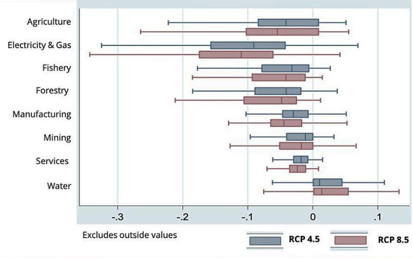
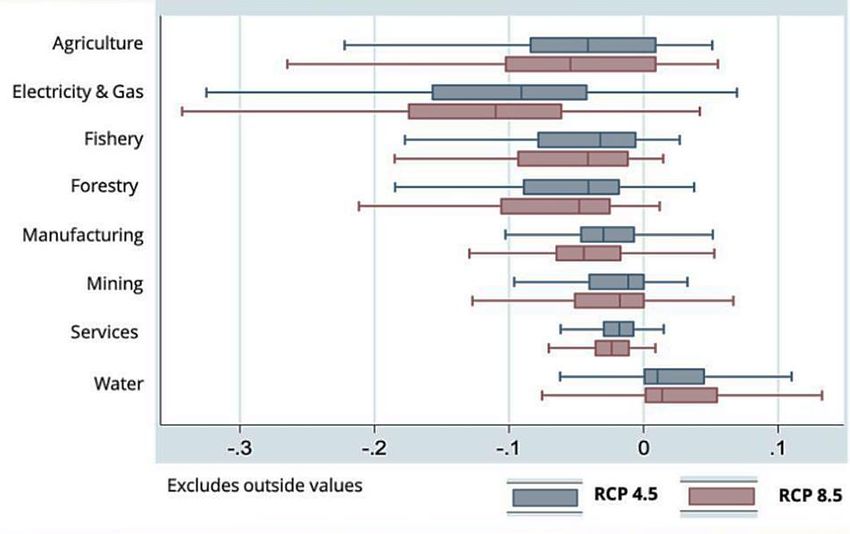
17Figure 3: Box plot of the distribution of sector-level effects
However, the projected effects for the different economic sectors and provinces vary a great
deal from municipality to municipality. A number of municipalities have a few positive extreme
values in all economic sectors. Nevertheless, apart from the water sector, the net effect for all
the sectors is negative, resulting in an average negative effect for the respective sectors and
the whole economy. From a policy point of view, watershed municipalities are therefore likely
to gain economically, while those relying on agriculture, forestry, fishery and electricity and
gas are likely to suffer the greatest losses. Policy attention should, therefore, focus on
adaptation in these sectors.
At the provincial level (shown in Table 5), the greatest impact of climate change will be felt in
Limpopo, where the RCP4.5 scenario will lead to 11% economic losses, while the RCP8.5 will
bring about 13% losses. This is in particular due to Limpopo’s high dependence on the
agriculture, forestry, fishery and electricity and gas sectors in which climate change effects will
be more severe in 2050. The next most significantly affected province is Mpumalanga, with its
main economic losses predicted to be in the agriculture (15%), forestry (12%), fishery (10%)
and electricity and gas (17%) sectors in the case of no mitigation assumptions. There is only
a 1% gain overall in Mpumalanga for the RCP4.5 mitigation scenario relative to RCP8.5. It is
worth noting that in the Western Cape, the average economic loss is predicted to be 3%, and
there is no difference between the RCP8.5 and the RCP4.5 mitigation scenarios. Of greater
18concern for this province, are the high relative losses predicted in the manufacturing sector.
Most of the provinces record positive effects in the water sector, except for the Western Cape
and the Northern Cape who will both be affected negatively in the water sector for RCP8.5,
with losses of 7% and 2% respectively. Apart from the water sector, there are a number of
other sectors that will be positively affected by climate change. For example, there will be an
8% gain in the mining sector in Mpumalanga due to climate change by 2030 for the RCP4.5
mitigation scenario (for RCP8.5 there will be a 10% gain). The Eastern Cape and Western
Cape agricultural sectors will experience a 2% increase related to climate change. In Gauteng,
the Free State, and the North West, the manufacturing sector will each expand by 2%. The
mining sector will also expand in the Free State and Gauteng by 1% each for the RCP8.5
scenario. In the Western Cape the fishery sector will expand by 1% due to climate change in
2030. The provincial findings suggest again that policy action for adaptation is most important
in the agricultural, forestry, fishery, and electricity and gas sectors in most provinces, but
particularly in Limpopo, Mpumalanga, and the Free State.
Table 5: Percentage losses/gains: Scenario 4.5 versus 8.5
Province Agri Man Min Ser For Fis E&G Wat All
Scenario RCP4.5
Eastern Cape 2 -3 -5 -2 -3 -3 -9 1 -3
Free State -6 2 1 -1 -11 -7 -12 3 -4
Gauteng -5 1 0 -2 -6 -6 -7 1 -3
KwaZulu-Natal -5 -3 -4 -2 -4 -5 -11 5 -3
Limpopo -22 -2 -4 -3 -22 -26 -18 5 -11
Mpumalanga -13 -3 8 -2 -10 -7 -14 0 -5
North West -4 2 -1 0 -4 -5 -8 1 -2
Northern Cape -6 -2 0 -3 -2 -1 -6 -1 -3
Western Cape 2 -8 -2 -2 -2 1 -6 -6 -3
National (%) -5.70 -2.25 -1.50 -1.98 -6.79 -5.97 -10.35 1.78 -4.10
Scenario RCP8.5
Eastern Cape 2 -4 -6 -3 -4 -4 -11 1 -4
Free State -7 2 1 -2 -13 -8 -15 4 -4
Gauteng -7 2 1 -3 -8 -9 -9 1 -4
KwaZulu-Natal -7 -3 -5 -2 -6 -6 -14 7 -4
Limpopo -27 -2 -5 -4 -28 -32 -23 6 -13
Mpumalanga -15 -4 10 -3 -12 -8 -17 1 -6
North West -5 2 -2 0 -5 -6 -9 1 -3
Northern Cape -7 -3 0 -4 -3 -2 -8 -2 -4
Western Cape 3 -9 -2 -3 -3 1 -7 -7 -3
National (%) -7.14 -2.77 -1.94 -2.49 -8.47 -7.26 -12.89 2.29 -5.08
19Figure 4: Box plot of the distribution of provincial effects
4.1.1 Key municipal findings
A number of individual municipalities present extreme effects in the positive and the negative
sides within specific sectors. The findings in these municipalities are summarised in Figure 5.
The most negative impact is in forestry in the Blouberg and Ephraim Mogale municipalities in
Limpopo with 50% and 48% losses respectively for the RCP4.5 scenario, and 54% and 47%
respectively for the RCP8.5 scenario. In order of decreasing magnitude of losses, key affected
municipalities are Mogalakwena in terms of fishery and agriculture, Mutale in agriculture,
forestry, and electricity and gas and Thulamela in agriculture and fishery. Other municipalities
to earmark for particular attention in adaptation policies are Elias Motsoaledi, Polokwane,
Makhuduthamaga, Greater Giyani, and Bela-Bela.
2040%
20%
0%
Blouberg
Mogalakwena
Mutale
Thulamela
Mutale
Mogalakwena
Blouberg
Makhuduthamaga
Greater Giyani
Bela-Bela
Polokwane
Mutale
Mogalakwena
Ephraim Mogale
Hlabisa
Mkhondo
Mtubatuba
Dr JS Moroka
Albert Luthuli
Mfolozi
-20%
-40%
RCP4.5 RCP8.5
-60%
Figure 5: Municipalities with extreme negative and positive effects
Positive effects are projected for a number of municipalities mainly in water and mining. In
Kwa-Zulu-Natal, uMfolozi has the highest gains in the water sector, followed by Ulundi,
Mtubatuba, and Hlabisa. A number of municipalities are projected to have positive effects in
the water sector in Limpopo. These are Ephraim Mogale and Mutale. In Mpumalanga, the
most significant positive effects are all in the mining sector for Msukaligwa, Chief Albert Luthuli,
Thembisile Hani, Dr JS Moroka, Thaba Chweu, Mkhondo, Lekwa, and Bushbuckridge.
5 RECOMMENDATIONS
Key recommendations in adapting South Africa’s settlements to climate change are:
RCP8.5 will yield significant economic losses.
Adaptation strategies have to be customised to suit specific socio-economic conditions
for a given settlement.
Settlement design has to take into account spatial inter-linkages in terms of economic
activities and anticipated climate change effects. This requires adaptation policy
coordination beyond local settlements to involve all spheres of government.
Careful human capital and skills development planning needs to account for the
structural effects of climate change and possible changes in trans-settlement linkages.
21Such plans have to be municipality- and/or province-specific, based on the anticipated
economic structural changes.
Adaptation strategies should emphasizes those settlements that rely on agriculture,
forestry and fisheries.
Settlements in the Limpopo, Mpumalanga and Free State provinces will be the most
vulnerable.
Settlement adaptation strategies should exploit opportunities that may arise in
expanding sectors, such as water in most provinces, and mining in Mpumalanga.
6 CONCLUSION
The projections of the effect of climate change have painted a picture, not only of significant
economic losses, but also of the potential to significantly alter economic structure. Certain
sectors are projected to expand in certain localities, such as mining in most of Mpumalanga
and the water sector in most of the country. However, losses outweigh gains in almost all
municipalities in South Africa. The implication of the findings is five-fold. First is that given the
international reluctance in committing to mitigation scenarios that will result in significantly low
radiation forcings, the most plausible forcing scenario will not be able to avert significant
economic losses. Therefore, adaptation strategies have to be put in place as urgently as
possible. The longer policy measures take to be implemented, the more losses are incurred
as the picture shows that we are already experiencing losses.
Given the varied effects by sector and by geography, adaptation strategies have to be
customised to suit specific conditions. Private economic agents may not be able to make
socially optimal choices in this regard, hence the need for careful public policy coordination
with significant state leadership.
The anticipated changes in economic structure imply that a number of sectors may shed jobs
in varying proportions. This highlights the need for careful human capital and skills
development planning that accounts for the economic structural effects of climate change.
Each municipality and/or provincial government will have to develop such plans based on its
anticipated economic structural change.
Climate change adaptable policies have to consider inter-municipal and inter-provincial
impacts. Our results suggest significant spatial effects of the impacts of climate change.
22Consequently, we suggest that policy measures must transcend cities to involve all tiers of
government with seamless coordination in order to deliver effective adaptation policy
implementation.
Main population groups to pay attention to in developing adaptation strategies should be those
that depend on agriculture, forestry and fisheries in most municipalities in almost all provinces,
especially in Limpopo, Mpumalanga, the Free State and the North West. Attention is to be
paid to the manufacturing sector in the Western Cape and the Eastern Cape, and to the water
sector in the Western Cape.
7 BIBLIOGRAPHY
Akram, N. and Hamid, A., 2015. Climate change: A threat to the economic growth of
Pakistan. Progress in Development Studies, 15(1), pp.73-86.
Alagidede, P., Adu, G. and Frimpong, P.B., 2016. The effect of climate change on economic
growth: evidence from Sub-Saharan Africa. Environmental Economics and Policy
Studies, 18(3), pp.417-436.
Benhin J. 2006. Climate change and South African agriculture: impacts and adaptation
options, CEEPA Discussion Paper No. 21 Special Series on Climate Change and
Agriculture in Africa ISBN 1-920160-01-09 Discussion Paper ISBN 1-920160-21-3,
July.
Brown, M.E., de Beurs, K. and Vrieling, A. 2010. The response of African land surface
phenology to large scale climate oscillations. Remote Sensing of Environment,
114(10), pp.2286-2296.
IPCC (2007) Report of the 26th session of the IPCC. Bangkok. April 30–May 4 2007.
Intergovernmental Panel on Climate Change, Geneva, Switzerland
Dell, M., Jones, B.F. and Olken, B.A., 2012. Temperature shocks and economic growth:
Evidence from the last half century. American Economic Journal: Macroeconomics,
4(3), pp.66-95.
Deschenes, O. and Moretti, E., 2007. Extreme Weather Events. Mortality and Migration.
NBER Working Paper, 14132.
23Golub, A. and Toman, M, 2015. Climate change, industrial transformation, and environment
growth traps. Environmental and Resource Economics 63(2):pp.249-263
Guiteras, R., 2009. The impact of climate change on Indian agriculture. Manuscript,
Department of Economics, University of Maryland, College Park, Maryland.
Jacob, B., Lefgren, L. and Moretti, E., 2007. The dynamics of criminal behaviour evidence
from weather shocks. Journal of Human resources, 42(3), pp.489-527.
Miguel, E., Satyanath, S. and Sergenti, E., 2004. Economic shocks and civil conflict: An
instrumental variables approach. Journal of political Economy, 112(4), pp.725-753.
National Planning Commission 2012. National Development Plan 2030 Our Future-make it
work, ISBN: 978-0-621-41180-5
OECD (2015), The Economic Consequences of Climate Change, OECD Publishing, Paris,
http://dx.doi.org/10.1787/9789264235410-en.
Statistics South Africa 2017. Gross Domestic Product, Second Quarter 2017. Statistical
Release P0441
Solow, R.M., 1956. A contribution to the theory of economic growth. The quarterly journal of
economics, 70(1), pp.65-94.
Tebaldi, E. and Beaudin, L., 2016. Climate change and economic growth in Brazil. Applied
Economics Letters, 23(5), pp.377-381.
US Library of Congress, 2006. South Africa. http://countrystudies.US/south_Africa/41.htm
and http://countrystudies.us/south-africa/67.htm
Van Vuuren, D., Edmonds, J., Kainuma, M., Riahi, K., Thomson, A. Hibbard, K., Hurtt, G.,
Kram , T., Krey, V., Jean-Francois Lamarque, J., Masui, T., Meinshausen, M.,
Nakicenovic, N., Smith, S. and Rose, S. 2011. The representative concentration
pathways: an overview, Climatic Change 109:5–31, DOI 10.1007/s10584-011-0148-z
Ziervogel, G., New, M., van Garderen, E., Midgley, G., Taylor,A., Hamann,R., Stuart-Hill,S.,
Myers, J. and Warburton, M. 2014. Climate change impacts and adaptation in South
Africa, WIREs Clim Change, 5:605–620. doi: 10.1002/wcc.295
24You can also read