The Effects of Police Violence on Inner-City Students
←
→
Page content transcription
If your browser does not render page correctly, please read the page content below
The Effects of Police Violence on Inner-City Students
                                         Desmond Ang∗
                                          June 7, 2020
                                              Abstract
           Nearly a thousand officer-involved killings occur each year in the United States.
       This paper documents the large, racially-disparate impacts of these events on the
       educational and psychological well-being of of public high school students in a large,
       urban school district. Exploiting hyperlocal variation in how close students live to a
       killing, I find that exposure to police violence leads to persistent decreases in GPA,
       increased incidence of emotional disturbance and lower rates of high school completion
       and college enrollment. These effects are driven entirely by black and Hispanic students
       in response to police killings of other minorities and are largest for incidents involving
       unarmed individuals.

   ∗
     Contact information: Harvard University, Kennedy School of Government, 79 John F. Kennedy St.,
Rubenstein 410, Cambridge, MA 02138, desmond ang@hks.harvard.edu. Word count: 14,053. I grate-
fully acknowledge financial support from the National Science Foundation. I thank Jim Andreoni, Kate
Antonovics, Julian Betts, Prashant Bharadwaj, Peter Blair, Michael Callen, Jeffrey Clemens, Gordon Dahl,
David Deming, Mitch Downey, Itzik Fadlon, Karthik Muralidharan, Charlie Sprenger and seminar partic-
ipants at UC San Diego, UC Riverside, University of Arizona, Dartmouth College, University of Chicago,
Harris, University of Illinois-Chicago, Tulane University, the National Bureau of Economic Research and
Harvard University for valuable feedback. Any errors are my own.
I       Introduction
    A central role of the state is to ensure public safety (Atkinson and Stiglitz, 2015). As
means of achieving this, American law enforcement officers are afforded broad discretion
over the use of force, and roughly a thousand individuals are killed by police each year.
In addition to protecting civilians from imminent harm, these incidents may help to deter
future criminal activity (Becker, 1968).
    At the same time, the four largest urban riots in recent American history were all triggered
by acts of police violence (DiPasquale and Glaeser, 1998).1 Experiences with aggressive
policing have been linked to unfavorable attitudes towards law enforcement, particularly
among racial minorities, whose lifetime odds of being killed by police are as high as one in
a thousand (Skolnick and Fyfe, 1993; Weitzer and Tuch, 2004; Brunson and Miller, 2005).2
These attitudes are, in turn, correlated with fear (Hale, 1996; Renauer, 2007; Boyd, 2018),
perceived discrimination (Brunson, 2007; Carr et al., 2007) and institutional distrust (Bobo
and Thompson, 2006; Kirk and Papachristos, 2011).
    Nonetheless, there exists little causal evidence of the social impacts of police use of force
on local communities. Correlational analysis of police violence and neighborhood health is
confounded by the fact that use of force is more likely to occur in disadvantaged areas, where
homicide and poverty rates are high (Kania and Mackey, 1977; Jacobs, 1998). Researchers
have attempted to address this issue by exploiting the timing of high-profile incidents: for
example, the police beatings of Rodney King in Los Angeles (Sigelman et al., 1997) and
Frank Jude in Milwaukee (Desmond et al., 2016) or the lethal shooting of Michael Brown
in Ferguson (Gershenson and Hayes, 2017).3 However, such landmark events were often
tipping points for larger social movements, like widespread riots in Los Angeles and Black
Lives Matter in Ferguson. Thus, their case studies may not be representative of the vast
majority of police killings that go unreported in the media and provide limited insight into
the day-to-day effects of use of force on nearby civilians. Furthermore, most existing studies
examine impacts on attitudes or interactions with law enforcement and are unable to shed
light on broader economic implications.
    This paper seeks to document the short and long-run consequences of police killings on the

    1
      These include: the 1965 Watts riots, the 1980 Miami riots, the 1992 Rodney King riots and the 2013
Ferguson riots. Police violence has also triggered large protests in other contexts. For example, in 2014, the
use of tear gas against students in Hong Kong sparked protests that blockaded roadways for several months.
    2
      Edwards et al. (2019) estimate that roughly one in 1,000 black men and one in 2,000 Hispanic men
will be killed by police over their life course, relative to one in 3,000 white men and one in 7,500 Asian
men. Among 25- to 29-year-old males, police violence is the sixth leading cause of death, behind accidents,
suicides, other homicides, heart disease and cancer.
    3
      Similarly, White et al. (2018) examine the impact of the Freddie Gray killing on perceptions of procedural
justice. The policy implications of those findings are discussed by Lacoe et al. (2018).

                                                       2
educational and psychological well-being of inner-city youth. I focus on high school students,
both because teenagers face crucial educational decisions and because studies suggest that
even vicarious police contact during adolescence may be influential in shaping long-run beliefs
and institutional trust (Winfree Jr and Griffith, 1977; Leiber et al., 1998; Hurst and Frank,
2000; Tyler et al., 2014).4
    To estimate these effects, I combine two highly detailed and novel datasets. The first
contains home addresses and individual-level panel data for all high school students enrolled
from 2002 to 2016 in a large urban school district in the Southwest (the “District”). The
second contains incident-level information on the universe of officer-involved killings in the
surrounding county (the “County”). By geo-coding the exact location of the 627 incidents
and over 700,000 home addresses, I am able to calculate each student’s precise geographic
proximity to police violence. Leveraging a dynamic difference-in-differences design, I then
exploit hyperlocal variation in the location and timing of police killings to compare changes
in well-being among students who lived very close to a killing to students from the same
neighborhood who lived slightly farther away.
    I find that acts of police violence have negative spillovers across a range of outcomes.
In the days immediately after a police killing, absenteeism spikes among nearby students.
Effects are largest for students who lived closest to the event and dissipate beyond 0.50
miles. This is consistent with the highly localized nature of police killings, nearly 80% of
which went unmentioned in local newspapers.
    In the medium-run, students living within half a mile of a police killing experience de-
creases in GPA as large as 0.08 standard deviations that persist for several semesters. That
these effects stem from exposure to a single officer-involved killing and that each killing af-
fects more than 300 students, on average, suggests the potentially traumatizing impact of
police violence. As corroboration, I find that exposed students are 15% more likely to be
classified with emotional disturbance – a chronic learning disability associated with PTSD
and depression – and twice as likely to report feeling unsafe in their neighborhoods the
following year.
    In the long-run, students exposed to officer-involved killings in the 9th grade are roughly
3.5% less likely to graduate from high school and 2.5% less likely to enroll in college. Though
smaller in magnitude, effects remain statistically and economically significant for students
exposed in the 10th and 11th grades.
    In unpacking the results, I document stark heterogeneity across race, both of the student
and of the person killed. The effects are driven entirely by black and Hispanic students in

   4
    Juveniles also experience far more frequent police interactions than other populations (Snyder et al.,
1996).

                                                    3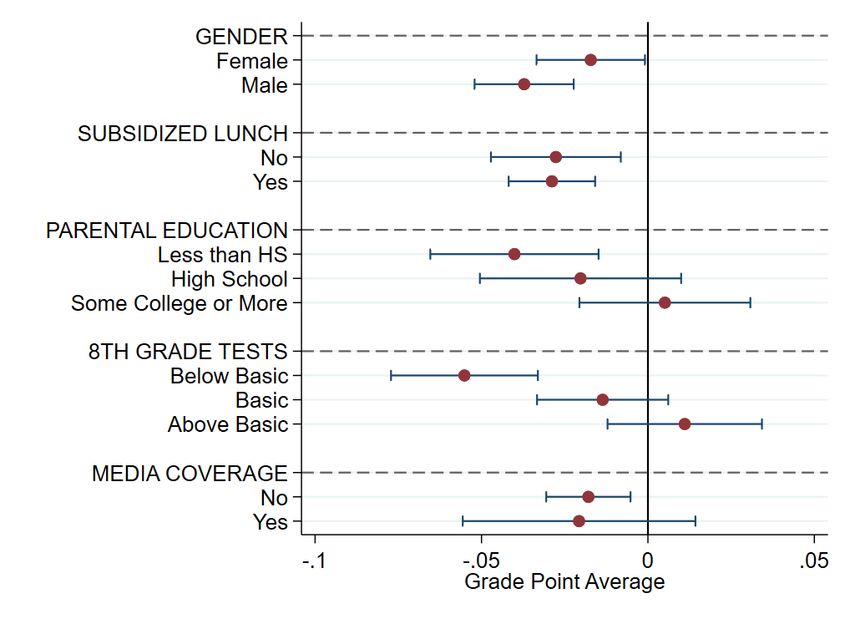
response to police killings of other underrepresented minorities. I find no significant impact
on white or Asian students. I also find no significant impact for police killings of white or
Asian suspects. These differences cannot be explained by other contextual factors correlated
with race, such as neighborhood characteristics, media coverage or other suspect and student
observables. However, the pattern of effects is consistent with large racial differences in
concerns about use of force and police legitimacy.5
    To further explore mechanisms, I exploit hand-coded contextual information drawn from
District Attorney incident reports and other sources. I find that police killings of unarmed
individuals generate negative spillovers that are roughly twice as large as killings of indi-
viduals armed with a gun or other weapon. This difference is statistically significant and
unattenuated when accounting for other observable suspect, neighborhood and contextual
factors. These findings suggest that student responses to police killings may be a function
not simply of violence or gunfire per se but also of the perceived “reasonableness” of officer
actions. Consistent with this, I find that the marginal effects of criminal homicides are only
half as large as those of police killings. Furthermore, unlike with police violence, the effects
do not vary with the race of the person killed. While students are only affected by police
killings of blacks and Hispanics, they respond similarly to criminal homicides of whites and
minorities.
    This paper makes four main contributions. First, it documents the large externalities
that police violence may have on local communities. My findings suggest that, on average,
each officer-involved killing in the County caused three students of color to drop out of
high school. As fatal shootings comprise less than one-tenth of one percent of all police
use of force encounters (Davis et al., 2018), this is likely a lower bound of the total social
costs of aggressive policing. While estimating the effects of less extreme uses of force is
complicated both by measurement error and by their relative prevalence, research suggests
that these interactions are also highly salient to local residents (Brunson and Miller, 2005;
Brunson, 2007; Legewie and Fagan, 2019) and are perhaps more likely to be exercised in a
racially-biased manner (Fryer Jr, 2019).6
    Second, this paper complements a growing body of research demonstrating how perceived

   5
      A 2015 survey found that 75% of black respondents and over 50% of Hispanic respondents felt police
violence against the public is a very or extremely serious issue, while only 20% of whites reported the same
(AP-NORC, 2015). Similarly, Bureau of Justice Statistics show that even conditional on experiencing force,
minorities are significantly more likely than whites to believe that police actions were excessive or improper
(Davis et al., 2018).
    6
      As Fryer Jr (2019) states, “data on lower level uses of force” are “virtually non-existent.” Causal
identification is further complicated by the fact that routine tactics like stop-and-frisk are often explicitly
determined by policing objectives and thus more likely to be endogenous with changes in neighborhood
conditions and law enforcement strategy.

                                                      4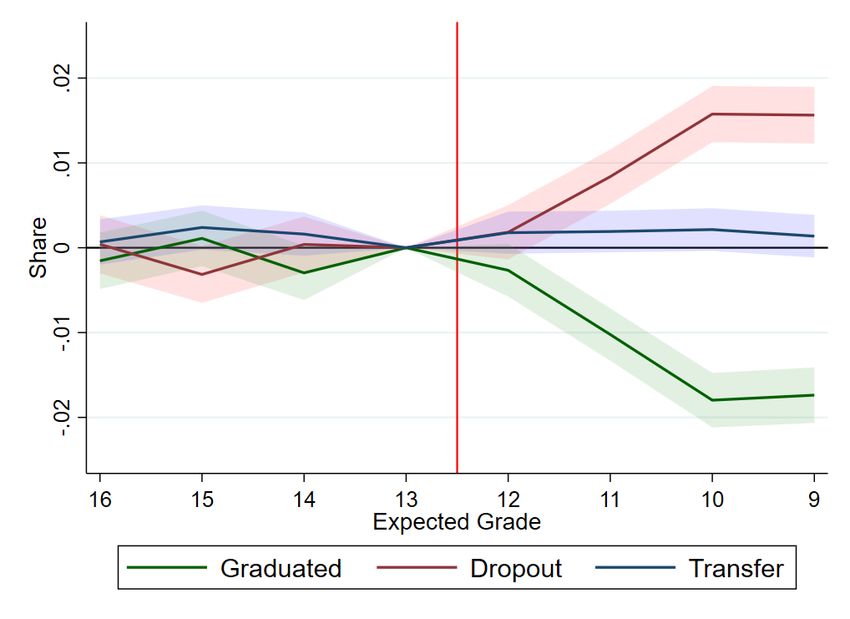
discrimination may lead to “self-fulfilling prophecies” in education (Carlana, 2019), labor
markets (Glover et al., 2017) and health care (Alsan and Wanamaker, 2018).7 . While empir-
ical evidence of racial bias is mixed (Fryer Jr, 2019; Nix et al., 2017; Knox and Mummolo,
2019; Johnson et al., 2019), the vast majority of blacks and Hispanics in America believe
that police discriminate in use of force (Pew Research Center, 2016, 2019; Dawson et al.,
1998; AP-NORC, 2015).8 Though more work is needed, the pattern of results suggests that
the educational spillovers of officer-involved killings may be driven in part by perceptions of
injustice surrounding these events.
    Third, this paper builds upon existing research measuring the short-run impacts of crim-
inal violence on children (Sharkey, 2010; Sharkey et al., 2012, 2014; Beland and Kim, 2016;
Rossin-Slater et al., 2019; Carrell and Hoekstra, 2010; Monteiro and Rocha, 2017; Gershen-
son and Tekin, 2017).9 However, in contrast to other forms of violence, the explicit purpose
of law enforcement is to improve public outcomes and the directional impact of aggressive
policing is ex ante far more ambiguous. Thus, my findings serve not simply as an exer-
cise in quantifying the costs of violence but rather as important inputs for pressing policy
discussions around police oversight and officer use of force.
    Finally, this paper provides further insight into the link between neighborhoods and
economic mobility (Katz et al., 2001; Chetty et al., 2016). Chetty et al. (2020) find that
intergenerational mobility differs dramatically between blacks and whites, even for children
from the same neighborhood and socioeconomic background. Consistent with research by
Derenoncourt (2018) documenting a negative correlation between police presence and black
upward mobility in Great Migration destinations, my results suggest that law enforcement
may play an important role in explaining this racial disparity. This is not only because mi-
norities are more likely than whites to experience police contact but also because, conditional
on contact, minorities may be more negatively affected by those interactions. Understanding
these effects and disentangling them from correlated factors like crime and poverty is critical
to the development of policies aimed at addressing persistent racial gaps across a wide range
of domains.
    The remainder of this paper is organized as follows: Section II describes the background
and data, Section III discusses the identification strategy and provides evidence of its validity,

   7
      It also relates to work by Chetty et al. (2020), who find that implicit bias measures and Google searches
of the “n” word strongly predict racial disparities in income mobility, and by Charles and Guryan (2008),
who find that General Social Survey measures of prejudice are correlated with black-white wage gaps in a
state.
    8
      For example, in a 2015 national survey, 85% of black respondents and 63% of Hispanic respondents
reported believing that police are more likely to use force against a black person. Similar shares reported
believing that police “deal more roughly with members of minority groups.”
    9
      Other work examines the impact of violence on other margins, like wages (Aizer, 2007).

                                                      5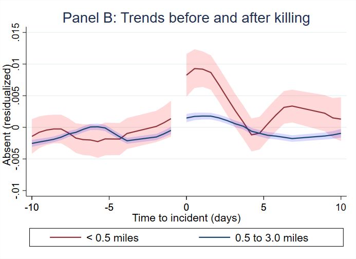
Section IV presents primary estimation results for academic achievement and psychological
well-being, Section V explores mechanisms by estimating differential effects by race and
incident context and by comparing the effects of police killings to criminal homicides, Section
VI examines long-run effects on educational attainment, and Section VII concludes.

II     Data
A    Police Killings Data
    Incident-level data on police killings come from a publicly available database compiled by
a local newspaper, which chronicles all deaths in the County committed by a “human hand.”
Whether an officer was responsible for the death is based on information from the coroner
and police agencies as well as from the newspaper’s own investigation. For each incident,
database records the name, age and race of the deceased as well as the exact address and
date of the event. In total, the data contains 627 incidents from July 2002 to June 2016.
    I supplement this data with contextual details drawn from District Attorney incident
reports. Each report includes a detailed description of the event based on forensic and
investigative evidence as well as officer and witness testimonies. Reports also provide a legal
analysis of officer actions. DA reports are not available for incidents that occurred prior to
2004 or that are still under investigation. For killings without DA reports, I searched for
incident details from police reports and other sources.
    Of the 627 sample incidents, I was able to obtain contextual information for 556 killings:
513 from DA reports and 43 from other sources. In each case, I read and hand-coded reports
to capture whether a weapon was recovered from the suspect and if so, what type. In cases
where a gun was found, I additionally captured whether the suspect had fired their weapon
at officers or civilians during the police encounter or immediately before (for example, in
cases where police were dispatched for an active shooter).
    It is worth noting that these measures provide an admittedly incomplete picture of the
surrounding events, which often involve imperfect information and split-second decisions.
In many cases, police actions were predicated on faulty or misreported information. For
example, in 2010, a woman called 911 to report that a man with a gun was sitting in her
apartment stairwell. Officers arrived and shot the man, but he was actually holding a water
hose nozzle. Similar situations arose when police were confronted by individuals armed with
firearms that turned out to be replicas. In other cases, killings were precipitated by seemingly
innocuous encounters that escalated unexpectedly. For instance, in 2014, patrol officers
attempted to stop a man for riding a bicycle on the sidewalk. Rather than complying, the

                                               6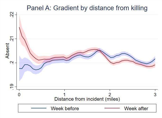
man grabbed an officer’s gun and was shot by the officer’s partner. Nonetheless, information
about weapon type and discharge has the benefit of being objectively verifiable and can be
found in all available incident reports. These details are also directly factored into legal
assessments of police actions as well as community perceptions of the “reasonableness” of
force (Brandl et al., 2001; Braga et al., 2014).
    Panel A of Table I provides a summary of the police killings data. 52% of suspects
were Hispanic, 26% were black, 19% were white and 3% were Asian.10 Relative to their
county population shares, black (Hispanic) individuals are roughly 4 (1.6) times more likely
to be killed by police than whites, who are in turn 3 times more likely to be killed than
Asians. The vast majority of individuals (97%) were male. The average age at death was
32 years old. Only 10% of individuals were of school age (i.e., 19 or younger) and none were
actively-enrolled District students.
    Consistent with national statistics, 54% of suspects were armed with a firearm (including
BB guns and replicas), while another 29% were armed with some other type of weapon.
This includes items like knives and pipes as well as cases in which the individual attempted
to hit someone with a vehicle. The remaining individuals, nearly 20% of the sample, were
completely unarmed. This is similar to the share of suspects who actively fired at officers
and civilians (22% of all suspects; 41% of gun-wielding suspects).
    Notably, the vast majority of incidents received little or no media coverage. Only 22%
of sample killings were ever mentioned in any of six local newspapers (including one of the
largest newspapers in the country) and only 13% were mentioned within 30 days of the
event.11 Conditional on being reported in a newspaper, the median number of articles is
two. Only two of the 627 incidents generated levels of media coverage anywhere near that
of recent nationally-reported killings.12
    Examining contextual factors separately by race, black and Hispanic suspects were
younger on average than white and Asian suspects (31 vs. 38 years old, respectively) and
more likely to possess a firearm (58% vs. 36%). However, rates of media coverage are iden-
tical between groups (22%), as are the median number of mentions, conditional on coverage.
    Regardless of demographics or circumstance, involved officers were rarely prosecuted. Of
the 627 incidents, the District Attorney pursued criminal charges against police in only one
case.13 This is consistent with national statistics, which find that criminal charges were filed

  10
      Race categories are mutually exclusive.
  11
      I searched for each incident by suspect name in six local newspapers. Combined, the papers circulate
roughly 1 million copies each day in the County and surrounding area.
   12
      Those killings were each cited in more than 200 articles. All other killings received fewer than 30
mentions.
   13
      Charges were not pressed in that instance until after the end of the sample period.

                                                    7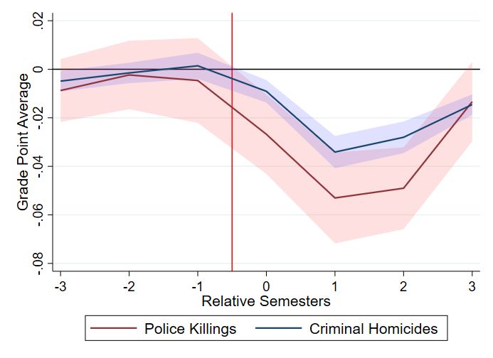
against police in fewer than half a percent of all officer-involved shootings.

B        Student Data
    The District administrative data contains individual-level records for all high school stu-
dents ever enrolled in the District from the 2002-2003 to 2015-2016 academic years. In total,
the dataset contains over 700,000 unique students. All student information is anonymized.
For each student, I have detailed demographic information including the student’s race,
gender, date of birth, parental education, home language, free/subsidized lunch status and
proficiency on 8th grade standardized tests. The data also contains each student’s last
reported home address while enrolled in the District.14
    The dataset includes a host of short and long-run measures of academic achievement.
Semester grade point average is calculated from student transcript data. I code letter grades
to numerical scores according to a 4.0 scale. I then average grades in math, science, English
and social sciences – the subjects used to determine graduation eligibility – by student-
semester to produce non-cumulative, semester grade point averages. Daily attendance for
every student is available from the 2009-2010 school year onwards. Each student-date ob-
servation contains the number of scheduled classes for which a student was absent that day.
This information is used construct a binary indicator for whether a student was absent for
any class on a given day (Whitney and Liu, 2017).15
    The primary measures of educational attainment are high school graduation and college
enrollment. Graduation is defined as receiving “a high school diploma or equivalent” from
the District.16 I am unable to distinguish between diploma types. Information on whether
students enrolled in post-secondary schooling is available for those that graduated from
the District between 2009 and 2014 and comes from the National Student Clearinghouse,
which provides enrollment information for institutions serving over 98% of all post-secondary
students in the country.
    The data also contains two sources of information regarding student mental health. From
the 2004 school year onwards, I observe the date students were designated by the District as
“emotionally disturbed,” a federally certified learning disability that “cannot be explained
by intellectual, sensory or health factors” and that qualifies for special education accom-
    14
      Because the data does not track previous addresses, I do not observe if a student moved within the
District. However, as I discuss in Section III, this is unlikely to be a serious source of bias.
   15
      Because attendance data is sometimes missing for some classes but not others within a given student-
date, using any absent classes requires less imputation. However, results are robust to coding absenteeism
based on all classes on a given date.
   16
      The dataset does not contain information on any years of schooling or diplomas that a student obtained
at high schools outside of the District. However, it does contain “leave codes” for students who transferred
out of the District before graduating, which allows me to test for differential attrition.

                                                     8
modations. This data is used to create student panel data indicating whether a student
was classified as “emotionally disturbed” in a given semester. The second source contains
student-level responses from a District-wide survey for the 2014-2015 and 2015-2016 academic
years. Of particular interest to this study, the survey includes three questions examining
feelings of school and neighborhood safety.17
Panel B of Table I provides summary statistics for the student data. The District is
comprised primarily of underrepresented minorities. 86% of students identify as either black
or Hispanic, while only 14% are white or Asian.18 The majority of students come from
disadvantaged households, with 69% qualifying for free or subsidized lunch and fewer than
10% with college-educated parents. Roughly 40% of students demonstrated basic or higher
levels of proficiency on 8th grade standardized tests.
Relative to the full sample, students who lived within 0.50 miles of an incident during high
school (i.e., the treatment group) are more likely to be Hispanic and to qualify for free lunch,
and less likely to speak English at home or to have college-educated parents. However, these
students look quite similar, on average, to students in the same Census block groups but more
than 0.50 miles away, who comprise the effective control group in my analysis.19 As shown in
the “Area” column of Table I, control students in treated neighborhoods come from similar
racial and household backgrounds as treated students, and are in fact, slightly less likely to
be proficient or to have college-educated parents. This similarity is an important feature
of the research design that helps to bolster internal validity, particularly when comparing
longer-run outcomes.
III Empirical Strategy
A Exposure to Police Killings
The primary obstacle to identification is that police killings are not random and may be
more likely to occur in disadvantaged neighborhoods where poverty and crime are high. Thus,
a cross-sectional comparison of students from parts of the County where police shootings are
relatively prevalent and students from parts of the County where they are not could be
confounded by correlated neighborhood characteristics. Furthermore, if changes in local
17
Responses are answered along a Likert scale ranging from one to five. While the survey is not mandatory,
it is typically administered during school hours leading to response rates above 75%.
18
Demographics differ from those of the county as a whole, which is comprised of approximately 48%
Hispanics, 9% blacks, 28% non-Hispanic whites and 14% Asian.
19
As my preferred estimating equation includes Census block group-semester fixed effects, causal identifi-
cation comes from comparing treatment and control students in the same Census block group, which average
roughly one square mile in area.
9poverty, crime or other unobserved factors predict police killings, biases could remain even
when including student fixed effects in panel analysis.
The address this, I exploit hyperlocal variation in exposure to killings within neighbor-
hoods. In essence, identifying variation comes from comparing changes over time among
students who lived very close to a police killing to students who lived slightly farther away
but in the same neighborhood. Thus, the two groups come from similar backgrounds and
were likely exposed to similar local conditions, except for the killing itself.
The plausibility of strategy is aided by two factors. The first is that police killings are
quite rare and difficult to predict. Over 300,000 arrests and nearly 60,000 violent crimes
occur in the County each year, compared to fewer than 50 officer-involved killings. Fur-
thermore, many police killings were entirely unaccompanied by violent crime. Roughly 20%
of incidents involved unarmed individuals, approximately the same share as those involving
armed suspects who fired at others. Thus, while underlying neighborhood conditions may
lead certain areas to experience more crime or to be more heavily policed, the exact timing
and location of officer-involved shootings within those neighborhoods is plausibly exogeneous.
The second factor in support of my empirical strategy is the under-reported nature of
police violence. In contrast to the handful of incidents that attracted national attention in
recent years, the vast majority of police killings received no media coverage. Thus, spatial
proximity is likely to be highly correlated with even learning about the existence of a police
killing. This provides meaningful treatment heterogeneity within neighborhoods.
Graphical Evidence
If students are affected by police killings, one might expect to see changes in school
attendance in the days following these events. If awareness of police killings is limited to
local communities or if the effects are otherwise correlated with geographic proximity (due
to social networks, visceral effects of witnessing the incident, etc.), then these changes should
dissipate with distance from the incident.
To test this, Figure I examines the raw absenteeism data. Panel A depicts the absenteeism
gradient of distance, separately for week before police killings and the week after (including
the incident date). Specifically, I estimate local polynomial regressions of daily absenteeism
on the distance between a student’s home and the incident location. The estimation sample
is comprised of the pooled set of observations within two weeks of each incident, where
distance and relative time are re-defined within each window.20
[Figure I about here.]
20
This analysis is restricted to killings from the 2009-2010 school year onward, the period for which daily
attendance data is available.
10The week prior to a killing, the gradient is relatively flat. That is, attendance patterns
for students who lived very close to where the event would occur are quite similar to those
who lived farther away. However, in the week after a police killing, absenteeism spikes among
nearby students. This uptick is largest for those who lived closest to the incident and fades
with distance. The pre- and post-killing gradients converge at around 0.50 miles and are
roughly parallel from there outward. These results are quite consistent with Chetty et al.
(2018), who find that “a child’s immediate surroundings – within about half a mile – are
responsible for almost all of the association between children’s outcomes and neighborhood
characteristics.”
Panel B of Figure I then depicts an event study of absenteeism, separately for students
who lived nearby (within 0.50 miles) and students who lived farther away (between 0.50
miles and 3.0 miles). I estimate local polynomial regressions of absenteeism (residualized by
calendar date) on the number of days before and after each event. In the days leading up
a police killing, absenteeism is virtually identical both in level and trend between the two
groups. In the immediate aftermath of these events, absenteeism increases sharply among
nearby students but remains smooth among those farther away.
Taken together, the two figures highlight the hyperlocal nature of exposure, suggesting
that students are affected by police killings that occur within 0.50 miles of their homes,
and that students living farther away may serve as a valid control for this group.21 They
also support the exogeneity of police killings. For these changes to be driven by unobserved
factors, one would have to believe that those confounds coincided with the exact dates and
locations of the police killings. Given that the full sample includes over 600 incidents spread
across fifteen years and thousands of square miles, this seems unlikely.
B Estimating Equation
To estimate effects on my primary measure of student performance – semester GPA –
I exploit the same spatial and temporal variation using a flexible difference-in-differences
(DD) framework. This model allows me to include individual fixed effects to account for
level differences between students as well as neighborhood-time fixed effects to control for
unobserved area trends or shocks, which may be of greater concern when examining outcomes
that are measured less frequently and over longer time horizons than daily attendance.
Drawing on the graphical evidence, the treatment group is comprised of students who
lived within 0.50 miles of any police killing that occurred during their District high school
career. On average, this captures 303 students per incident. Roughly 20% of the sample is
21
As I will demonstrate in the Section IV, the flatness of the distant gradient also suggests that estimation
results are insensitive to the choice of control bandwidth beyond 0.50 miles.
11ever-treated based on this definition. The control group consists of students whose nearest
police killing during their District tenure was between 0.50 miles and 3 miles away from their
home. As I will demonstrate later, estimates are insensitive to alternative definitions of the
control group, but increase in magnitude as the treatment bandwidth narrows to students
living closest to a killing.
I then estimate the following base equation on the student panel data:
X
(1) yi,t = δi + λn,t + ωc,t + βτ Shootτ + i,t ,
τ 6=−1
where yi,t represents semester GPA of individual i at semester t. δi are individual fixed effects
and λn,t are neighborhood-semester fixed effects. In my primary specification, neighborhood
is defined by Census block group, which measure roughly one square mile in area. ωc,t are
cohort-year fixed effects, which account for grade inflation as students progress through high
school. Shootτ are relative time to treatment indicators, which are set to 1 for treatment
students if time t is τ periods from treatment.22 For the 15% of treatment students who
were exposed to multiple killings during their high school tenure, treatment is defined by
the earliest nearby killing.23 The coefficients of interest (βτ ) then represent the average
change between time τ and the last period before treatment among students exposed to
police violence relative to that same change over time among unexposed students in the
same neighborhood. Drawing on Bertrand et al. (2004), standard errors are clustered by zip
code, allowing for correlation of errors over time within each of the sample’s 219 zip codes.24
Crime and Policing
A primary threat to identification is that unobserved changes in local crime or policing
activity may explain both the presence of police shootings and changes in academic perfor-
mance. However, because I am able to account for time trends at the neighborhood-level,
any potential biases would have to be hyperlocal, differentially affecting students in the
same Census block group. To test this, I use a block-level analogue of Equation 1 to exam-
ine whether Census blocks that experienced police killings also saw differential changes in
homicides, crimes or arrests in the prior or following semesters.25
22
Killings from January to June are mapped to the spring semester, while those from July to December
are mapped to the fall semester.
23
In robustness analysis, I also drop students exposed to multiple killings and find similar results.
24
As shown in the Appendix, results are robust to different methods of calculating standard errors, such
as clustering by school or Census tract and multi-way clustering by zip code and time (Cameron et al., 2012).
25
While data on homicides is available for the entire sample, information for arrests and non-homicide
crimes is only available from 2010 onwards.
12These results are shown in Appendix Figure A.I. In each case, I find little evidence of
differential trends prior to police shootings. This supports the plausible exogeneity of police
killings, after conditioning on block group-time. Following acts of police violence, I also find
little evidence of differential changes in crimes or arrests between the streets where those
incidents occurred and other areas in the same neighborhood. Point estimates for reported
crimes never exceed 0.31 in magnitude, less than 10% of the sample mean (3.16 reported
crimes per block-semester). Furthermore, six of the eight post-treatment estimates are neg-
ative. Thus, if local crime and student performance are negatively correlated, potential
biases would drive treatment estimates for GPA upwards (i.e., towards zero). Similarly, all
post-treatment estimates for homicides and arrests are insignificant and more than half are
negative in sign.
This does not mean that police violence has no impact on crime. It is possible that
the deterrence effects of police shootings are not localized to the specific blocks in which
they occur, but are instead distributed throughout an entire precinct or city. These changes
would then be absorbed by the neighborhood-time fixed effects in the difference-in-differences
model. While a thorough investigation of the relationship between police use of force and
crime is outside the scope of this paper, these findings reinforce the exogeneity of police
killings and demonstrate that differential shocks in local crime or policing activity are unlikely
to bias my treatment estimates.26
Selective Migration
Another potential threat is selective migration, as exposure to police violence may cause
treated students to relocate or drop out of school. The latter is an outcome of interest in its
own right, which I will examine directly in Section VI. Of greater concern are students who
relocate within the county while remaining enrolled at the District. Because the data only
contains a student’s most recent address, students who were exposed to violence at their
previous addresses may be incorrectly marked as control, or vice versa.
However, 2006-2010 ACS data suggests that any measurement error is uncorrelated with
treatment and would simply bias my estimates towards zero. 86.6% of individuals living in
Census block groups where a police shooting occurred reported residing at the same house
one year prior, virtually identical to the 86.8% tenure rate among those living in block groups
that did not experience a shooting (p = 0.628). Even if measurement error was correlated
with treatment, the inclusion of student fixed effects would account for any level biases that
might arise due to migration – such as if high-achieving students were more likely to re-locate
26
As corroboration, results in Section IV show that my primary treatment estimates are robust to directly
controlling for homicides, crime and arrests.
13following exposure.27
IV Main Results
A Academic Performance
I first examine the effects of exposure to police killings on academic performance by
estimating Equation 1 on semester GPA. The omitted period is the last semester prior to
treatment. Estimates are displayed in Figure II.
[Figure II about here.]
Prior to shootings, I find little evidence of differential group trends. For τ < 0, all
treatment coefficients are less than 0.012 points in magnitude and never reach statistical sig-
nificance, even at the 10 percent level. Pre-treatment estimates are also jointly insignificant
(F = 0.69, p = 0.655). This is consistent with the exogeneity of police killings, which are
rare events that are not preceded by observable changes in local crime or policing activity.
Following shootings, grade point average decreases significantly among students living
nearby. GPA declines by 0.04 points in the semester of the shooting and by between 0.07
and 0.08 points in the following two semesters (GPA mean=2.08, SD=1). Effects then
gradually dissipate, reaching insignificance five semesters after exposure. As I will discuss
in Section VI, this does not mean that there are no long-run effects of exposure. If police
violence causes affected students to drop out, treatment estimates on semester GPA would
mechanically converge to zero as relative time increases.28
To place these effects in context, the mean post-treatment estimate of -0.030 SD is larger
in absolute magnitude than the average impact of randomized interventions providing stu-
dent incentives (0.024 SD), low-dosage tutoring (0.015 SD) and school choice/vouchers (0.024
SD) found in the literature (Fryer Jr, 2017). Alternatively, the observed effects predict a
roughly 1.5 percentage point decrease in graduation rate, suggesting that changes in achieve-
ment may have significant consequences for long-run educational attainment.
Figure III presents results from estimation using alternative definitions of treatment and
control groups. In Panel A, I vary the control bandwidth, holding fixed treatment at 0.50
27
While this does not rule out the existence of other forms of non-classical measurement error, the data
suggests that intra-county migration is unlikely to be a serious confound. In Appendix Figure A.II, I find
limited evidence of increased intra-District transfers among schools that experienced police killings in their
catchment zones, as would be expected if shootings caused students to move to safer neighborhoods.
28
Additionally, if affected students are tracked into less rigorous classes, grades could rise even if academic
performance or aptitude remains depressed.
14miles. Results are highly stable as the control group shrinks from students living within 3
miles of a killing to those living within 1 or 2 miles from an incident. This is consistent
with the absenteeism figures, which found relatively flat gradients of distance in student
attendance beyond 0.50 miles, and demonstrates robustness to the choice of control group.
[Figure III about here.]
In Panel B, I instead vary the treatment bandwidth, defining exposure at 0.25, 0.375 and
0.50 miles. In all cases, the control group is comprised of students living between 0.50 and 3
miles from an incident. Again, I find little evidence of differential pre-trends and significant
decreases in GPA coinciding with exposure to police killings. However, comparing results
across models, magnitudes increase monotonically as the treatment bandwidth is tightened.
Estimates for the semester after treatment rise from 0.08 points when exposure is defined at
one-half mile, to 0.11 points at three-eighths of a mile and 0.16 points at one-quarter mile.
This is again consistent with the absenteeism figures and suggests that students living
closest to police killings are most detrimentally affected. In light of the under-reported nature
of these events, one explanation for the localized effects may be differences in information.
That is, individuals living more than a few blocks from a killing may be completely unaware
of its existence. It is also possible that even among students that knew about an incident,
those that personally knew the suspect or directly witnessed the violence may be more
negatively impacted.
Though I cannot fully disentangle these two channels, Appendix Figure A.III compares
average treatment effects for police killings that received media coverage and those that did
not. I find nearly identical point estimates in each case, suggesting that more widely-known
incidents do not necessarily have larger educational spillovers among local residents. Given
that only 15 percent of media-covered incidents were mentioned in more than five newspaper
articles, one explanation for the similar effects is that my measure of media coverage is only
weakly correlated with information dissemination. However, as I discuss in Section V, effect
sizes do increase with the demographic similarity of students and suspects, suggesting that
informal networks or personal affiliation may be a more salient mediating channel.
The remainder of Figure A.III contains other heterogeneity analysis. I recover larger
treatment estimates for male students as well as for students with less educated parents or
lower 8th grade test scores, suggesting that lower-achieving and more disadvantaged students
may be most affected by exposure to police killings. It is also possible that these differential
impacts are driven in part by racial heterogeneity, which I will explore in detail in Section
V.
15Robustness
Panel A of Table II demonstrates robustness to a host of alternative specifications. Col-
umn 1 presents my preferred specification using a simple post-treatment dummy. To address
possible biases due to local crime, Column 2 adds controls for the number of criminal homi-
cides in a Census block-semester. In Column 3, I additionally add time-varying controls for
the number of arrests and reported crimes in a block, restricting the sample to 2010 onwards
(i.e., the period when crime and arrests data are available). To test robustness to alternative
definitions of neighborhood, Column 4 replaces the semester by Census block group fixed
effects with semester by Census tract fixed effects (there are roughly 2.6 block groups per
tract). Column 5 instead controls for neighborhood time trends using arbitrary square-mile
units obtained from dividing the County into a grid. To demonstrate that the effects are not
driven by multiply-treated students, Column 6 drops the 15% of treatment students that
were exposed to more than one police killing. To address potential differential migration
into the sample, Column 7 drops students that first entered the District in the 10th to 12th
grades. In all cases, I recover similar average treatment effects on student GPA of around
-0.20 to -0.30 points.
[Table II about here.]
The Appendix contains additional robustness checks and analysis. Table A.I shows results
using alternative calculations of standard errors (i.e., multi-way clustering with zip code and
year and clustering by school catchment or tract). In all cases, I recover similar results with
insignificant estimates prior to treatment and highly significant estimates in the semesters
following police killings. As the paper’s primary estimates pool across students exposed at
different grades, Figure A.IV replicates the analysis separately for students exposed in the
9th, 10th, 11th and 12th grades and finds that exposure to police violence leads to decreased
GPA across each subsample.
To test whether the documented effects are specific to the timing and location of the
sample incidents, I run a series of permutation tests. In each regression, I first randomize
the location and date of 627 placebo killings within the sample area and period. Treatment
and control groups are generated as before and average treatment effects are estimated using
Equation 1 and a single post-treatment dummy. Figure A.V presents a histogram of the
coefficient of interest for each of 250 tests. The red vertical line benchmarks the estimated
coefficient using the true sample. Of the 250 placebo regressions, only four produce estimates
greater in absolute value than the true estimate of -0.027 points.
16B Psychological Well-Being
I next explore effects on psychological well-being using data on clinical diagnoses of emo-
tional disturbance. Emotional disturbance (ED) is a federally certified disability defined as
a “general pervasive mood of unhappiness or depression,” “a tendency to develop physical
symptoms or fears,” or “an inability to learn,” which “cannot be explained by intellectual,
sensory, or health factors.” While there is no single cause of emotional disturbance, its symp-
tomatology and incidence are strongly linked with post-traumatic stress disorder (Mueser
and Taub, 2008). Figure IV displays results from estimation of Equation 1 on incidence of
ED under my preferred specification.
[Figure IV about here.]
I find little evidence of differential pre-trends between treatment and control students
(F-test of joint significance: F = 1.15, p = 0.334). However, students exposed to police
violence are significantly more likely to be classified as emotionally disturbed in the following
semesters. Though the treatment estimates are small, ranging from 0.04 to 0.07 percentage
points, they are highly significant and represent a 15% increase over the mean (0.5% of
sample students are classified with ED in a given year). As demonstration of robustness,
Panel B of Table II shows similar effects under alternative specifications.
Changes in emotional disturbance are also highly persistent with little drop-off several
semesters after exposure. This is likely due to two factors. First, emotional disturbance
and psychological trauma are chronic conditions and often last for several years after the
inciting incident (Friedman et al., 1996; Famularo et al., 1996). Second, ED designations
are sticky. While designations are reviewed by the District each year, comprehensive re-
evaluations are only required every three years. Thus, the drop-off in effect observed seven
semesters after treatment coincides precisely with the timing of triennial re-evaluations for
students diagnosed shortly after exposure.
While these results are consistent with the possible traumatizing effects of police violence,
they could also be driven by changes in school reporting or detection of ED rather than actual
incidence of it. However, as shown in Appendix Table A.II, I find that exposure to police
killings also leads to changes in self-reported feelings of safety. In particular, nearby students
are twice as likely to report feeling unsafe outside of school the year after a killing. This
analysis, which draws on responses from the District’s annual survey, suggests that exposure
to police violence does impact students’ underlying psychological well-being. It also provides
causal evidence in support of recent work by Bor et al. (2018), who examine cross-sectional
survey data and find that police killings of blacks are linked to lower self-reported mental
17health among black men living in the same state.29
Given that students are not regularly screened for ED and designations are only made
after an intensive referral process, these estimates likely represent a lower bound of the true
psychological impacts of police violence.30 Epidemiological studies estimate that between 8%
and 12% of all adolescents suffer from some form of emotional disturbance (U.S. Department
of Education, 1993) — more than fifteen times the diagnosed rate among District students.
The results also provide important insight into the observed effects on academic per-
formance. Consistent with recent work demonstrating that violence affects cortisol levels
(Heissel et al., 2018) and that cortisol predicts test performance (Heissel et al., 2018), my
findings suggest that decreases in GPA may be driven in part by psychological trauma.
However, in addition to maintaining worse grades than their peers (Wagner, 1995), students
with ED are 50% less likely to graduate and significantly more likely to suffer from low self-
esteem and feelings of worthlessness, suggesting that the long-run effects of police violence
may extend beyond in-class performance (Beck et al., 1996; Carter et al., 2006).31
V Mechanisms
To better understand the mechanisms behind these effects, I exploit rich heterogeneity
in the data. Given large racial differences in attitudes towards law enforcement as well as
significant variation in the police killings themselves, I explore heterogeneous effects by race
and incident context. I then directly compare the effects of police use of force to those of
criminal homicides.
A Racial Differences
I first explore differential responses by race. I estimate Equation 1 on GPA, separately
for each race subsample. For sake of power, I pool white and Asian students together. Panel
A of Figure V displays treatment coefficients for a simple post-treatment dummy.
[Figure V about here.]
29
Similarly, work by Moya (2018) and Callen et al. (2014) demonstrates that exposure to violence more
generally may lead to changes in risk aversion. Rossin-Slater et al. (2019) find that youth anti-depressant
use increases following local school shootings.
30
Students are only classified as ED after 1) pre-referral interventions have failed, 2) referral to Special
Education and 3) a comprehensive meeting between the student’s parent, teachers and school psychologist.
This process can be quite costly to the District, as students with ED often receive their own classrooms and
are sometimes transferred to private schools or residential facilities at the District’s expense.
31
Emotional disturbance is also associated with limited attention spans (McInerney et al., 1992) and
impaired cognitive functioning (Yehuda et al., 2004)
18As shown, I find stark differences in effects by student race. Black and Hispanic students
are significantly affected by police killings and experience average GPA decreases of 0.038
and 0.030 points, respectively. However, exposure to police killings has no impact on white
and Asian students with a treatment coefficient of essentially zero (-0.003 points).
One possible explanation for the differing effects by student race is that black and His-
panic students may come from more disadvantaged backgrounds. Given earlier evidence of
heterogeneous effects by parental education and 8th grade achievement, those same factors
could potentially account for the results found here.
To test this, I create a new sample of black and Hispanic students that matches the
distribution of the white and Asian students. I match the former set of students to the
latter based on free lunch qualification, parental education (HS degree, less than HS, more
than HS), 8th grade standardized test score (by pentile), cohort (within 3 years) and school.
To maximize power, I randomly select up to 8 black or Hispanic student per each white
or Asian student and weight observations by one over the number of matches to maintain
sample balance on match characteristics. Table A.III provides a descriptive comparison of the
matched and unmatched samples as well as estimation results for each. Notably, estimated
effects for the original minority sample are quite similar to those for the re-weighted minority
sample (-0.031 points vs. -0.029 points) and both are far larger than the zero estimate
for the white sample. This suggests that differences in family background, prior academic
achievement, school and cohort explain very little of the gap in minority and non-minority
responses to police killings.
These results provide evidence of the disproportionate burden police violence may have on
underrepresented minorities, even conditioning on exposure. This is consistent with work by
Gershenson and Hayes (2017), who examine the 2013 Ferguson riots and find that test score
decreases were largest in majority-black schools. It is also consistent with a host of research
demonstrating that race is the single strongest predictor of perceptions of law enforcement
(Taylor et al., 2001). Even controlling for other factors, blacks and Hispanics are significantly
more likely to believe that police use of force is excessive or unjustified (Weitzer and Tuch,
2002; Leiber et al., 1998).
A similar pattern emerges when examining heterogeneity by suspect race. As shown in
Panel B of Figure V, killings of black and Hispanic suspects have significant spillovers on
academic achievement (-0.031 points and -0.021 points, respectively). This is not true of
incidents involving white or Asian fatalities.32 The treatment estimate for killings of whites
and Asians is essentially zero (0.003 points).
32
Given that Asians comprise only 3% of the police killings sample, I again pool those individuals with
whites.
19In interpreting these results it is important to note that suspect race is obviously not
randomly assigned. Thus, while police killings of blacks and Hispanics exert demonstrably
larger effects than killings of whites and Asians, these differences could be driven by factors
correlated with suspect race rather than race itself. For example, it is possible that the
former are particularly harmful because they occur in more disadvantaged areas or because
the person killed was more likely to have been from the neighborhood or known in the
community.
Thus, to better understand the salience of suspect race, I introduce flexible controls
allowing for differential treatment effects along a range of neighborhood, incident and suspect
characteristics. In particular, I estimate the following equation on the full sample:
(2)
yi,t =δi + λn,t + ωc,t + βBH P ost × Shoot × BlackHispanic + βW A P ost × Shoot × W hiteAsian
+ P ost × Shoot × Xi γ + i,t ,
where Xi is a vector of controls that may be correlated with suspect race. Controls are
interacted with post-treatment indicators to absorb variation in treatment effects associated
with those factors. The inclusion of these controls means that βBH and βW A no longer repre-
sent the average treatment effects of black/Hispanic and white/Asian killings, respectively.
Instead, estimated treatment effects are obtained from a linear combination of βBH , βW A
and γ. Nonetheless, the difference between βBH and βW A is informative of the remaining
variation in treatment effects attributable to suspect race and provides insight into the rel-
evant counterfactual: all else equal, how would students have responded if the person killed
was of a different race?
[Table III about here.]
Table III displays estimated treatment effects from estimation of Equation 2 under various
specifications. Column 1 shows results from my base specification without any controls. Con-
sistent with the subsample analysis, I find large and significant estimates for black/Hispanic
killings and small, insignificant estimates for white/Asian killings. To account for the possi-
bility that killings in more disadvantaged neighborhoods produce larger spillovers, Column
2 controls for population density, non-white population share, homicide rate and average
income in a student’s Census block group. Column 3 further accounts for informational
differences that may exist between black/Hispanic and white/Asian killings. In particular,
I control for whether the incident occurred near the suspect’s home and for whether it was
mentioned in a local newspaper, as students may be more affected by killings that involved
20You can also read