The Impact of Clean Water on Infant Mortality: Evidence from Piped Water Provision in China

The Impact of Clean Water on Infant Mortality: Evidence from Piped
 Water Provision in China

 Maoyong Fan and Guojun He *

 September 2020

 Abstract
We examine the impact of clean drinking water on infant mortality in China using a novel
instrumental variable: the least-cost distance between water sources and infant mortality
surveillance areas. We find that provision of piped water significantly decreases infant
mortality, with a 10 percentage-point increase in piped water reducing infant mortality by
16 percent. Access to piped water is particularly beneficial in rural areas, and in regions
with marginally polluted surface waters. The economic benefits of piped water provision
in rural China outweigh the estimated costs.

Keywords: Clean Drinking Water, Piped Water, Infant Health, Child Mortality, Water
Pollution

JEL Classification: I15 I18 J10 Q53 Q56

*
 Fan: Department of Economics, Ball State University, Muncie, IN, USA (mfan@bsu.edu). He: Division of Social
Science, Division of Environment, and Department of Economics, The Hong Kong University of Science and
Technology, Hong Kong, China, (gjhe@ust.hk).
Acknowledgement: We thank participants in seminars and workshops at Ball State University, Indiana University,
Nankai University, Tongji University, AAEA Annual Meeting, CES North American Annual Conference, HKEA 10th
Biennial Conference, CEC Economics Research Workshop. An Xue from Peking University provides valuable help for
calculating least cost distance. Wenwei Peng and Lanyu Zhu offered excellent research assistance. The project is partially
funded by the General Research Fund (26500016) of HK Government.

I. Introduction

Clean drinking water is essential to human health. It is estimated that in 2015 about 663
million people worldwide still lacked basic water service, and among them almost 159
million people consume untreated water directly from rivers, lakes, and other surface water
sources (UNICEF, 2015). Untreated water sources are a major cause of infant mortality
and morbidity. An estimated 1,800 children under the age of five die every day from
diseases linked to water, sanitation, and hygiene in the world (UNICEF, 2015).
 The World Bank estimated that China reduced its infant mortality rate by more than
two thirds from 30.1 per 1,000 livebirths to 9.2 per 1,000 livebirths between 2000 and
2015. 2 Part of this reduction was due to a massive investment made by the Chinese
government in clean water infrastructure: the piped water coverage in rural areas has
expanded by approximately 60% between 2000 and 2010. While it is commonly perceived
that the improved access to clean water is a major contributor to lower mortality rates
among infants (WHO, 2009), no studies have quantified the magnitude of the benefits that
piped water provided in improving infant health (e.g. mortality) in China.
 In this study, we estimate the impact of piped water provision on infant mortality
in China. We have compiled what is to our knowledge the most comprehensive assessment
of clean water access, infant mortality, and surface water quality in China ever assembled.
The household-level piped water access is aggregated to the county level. These data are
linked to the infant mortality data from China’s Ministry of Health, a nationally-
representative sample that tracks all infant deaths among inhabitants in 331 Chinese
counties and city districts. By combining these two data sets, we are able to examine an
accurate sample of mortality and clean water access at a level of quality not commonly
found in developing countries. By combining both digital and print resources, we also
assembled a data set of surface water quality taken across over 800 monitoring stations.
 A simple comparison of outcomes in areas with high and low piped water coverage
is unlikely to provide a causal estimate of the impact, because piped water coverage is

2
 The infant mortality estimates are developed by the UN Inter-agency Group for Child Mortality Estimation
(UNICEF, WHO, World Bank, UN DESA Population Division ) at childmortality.org. The data are available
at https://data.worldbank.org/indicator/SP.DYN.IMRT.IN?locations=CN. Last accessed date: Nov. 16, 2018.
 1

determined by many socio-economic factors that may as well affect infant mortality. To
address the endogeneity concerns of piped water coverage, we construct a novel
instrumental variable based on the least-cost route from water sources to destinations using
GIS network analysis. Because constructing water pipelines are costly, and the costs
depend critically on the geographical characteristics between a surveillance area (where
infant mortality data are gathered) and its nearby clean water sources (e.g. reservoirs), we
can use the least-cost distance between them as the instrument for piped water coverage.
Since the least-cost path is constructed purely based on cost considerations, it should be
uncorrelated with demand-side determinants of infant mortality (such as income and social
preferences).
 We focus on infant mortality for three reasons. First, infants are particularly
vulnerable to environmental risks because their immune and other bodily systems are still
developing. As an example, because of differences in body mass/size, polluted water
carrying pathogens that cause diarrhea can lead to dehydration and death in infants within
hours, while the same infection would be much less serious to adults. Second, the exposure-
effect relationship is more immediate for infants, whereas for adults, diseases may reflect
pollution exposure accrued over many years. Focusing on infants provides a clean setting
for estimating the health effect of pollution (Chay & Greenstone, 2003a, 2003b; Currie,
Graff Zivin, Meckel, Neidell, & Schlenker, 2013; Currie & Neidell, 2005; Currie, Neidell,
& Schmieder, 2009). Third, compared with older cohorts, saving infant lives generates
larger social benefits in terms of life expectancy and productivity. A growing body of
research suggests that early-life health status affects long-term economic outcomes, such
as human capital accumulation, labor force participation, and earnings (Currie & Almond,
2011). Therefore, policymakers are often highly motivated to reduce infant mortality.
 We make several contributions to the literature. First, this study is the first national
research on clean water and infant health in China. We have compiled what is to our
knowledge the most comprehensive assessment of piped water access, surface water
pollution, and infant mortality in China ever assembled. By combining these three data sets,
we are able to examine an accurate sample of infant mortality and clean drinking water at
a level of quality rarely found in developing countries. In contrast, most of the existing
literature focuses on specific geographical regions. Furthermore, previous studies

 2

commonly use an aggregated infant mortality measure as the outcome and fail to examine
the potential differential impacts on different causes of deaths. The infant mortality data in
this study contain detailed information on different causes of death and allow us to examine
what diseases are particularly sensitive to water contamination and better understand the
pathological causes of infant mortality.
 Second, we identify the effect using a novel instrumental variable and show that
the least-cost path between the infant mortality surveillance areas and their nearby water
sources is likely to be a valid instrument: 1) it is a strong predictor of piped water coverage,
and 2) it is uncorrelated with a rich set of health-influencing variables (such as income,
public health expenditure, availability of medical services, etc.) that are important
determinants of infant mortality. As we rely on cross-sectional variations to identify the
health impacts of piped water provision, knowing that the instrument is uncorrelated with
the observed health determinants significantly alleviates the potential endogeneity
concerns.
 Third, combining surface water pollution and piped water coverage, we explore the
interactions between them by examining the impact heterogeneity across regions with
different levels of water pollution and highlight areas in which piped water provision is
particularly important for infant health. We find that the effect of piped water provision is
greater in regions with slightly polluted surface water rather than in regions with severely
polluted water. This is likely because when rivers and lakes become severely polluted and
the pollution becomes noticeable, people will stop consuming the surface water. However,
slightly polluted surface water is often mistakenly deemed clean and consumed if people
cannot access piped water and have little knowledge about the levels of water pollution. In
addition, we also find the effect of piped water provision on infant mortality is greater in
rural areas. Therefore, increasing piped water coverage in slighted polluted and rural areas
will likely generate greater health and economic benefits.
 Despite the dramatic decline in infant mortality in the past few decades, China still
has substantial disparities in infant mortality across different regions. In 2010, the infant
mortality rate in some rural counties was still as high as 50 per thousand live births, while
in some urban areas it was lower than 1 per thousand live births. The data show similar
heterogeneity for piped water coverage. The mean piped water coverage in rural counties

 3

was 55% in 2010 with a standard deviation of 24%. The highest piped water coverage was
close to 100%, but the lowest coverage rate was less than 1%. Given the enormous costs
of building and maintaining the piped water infrastructure, in order to formulate optimal
economic policies, it is crucial to quantify the benefits of such investments. Based on our
empirical results, we conduct an exploratory cost and benefit analysis for expanding piped
water infrastructure in rural areas and show that the benefits of piped water provision
significantly outweigh its costs. Therefore, further expansion of piped water coverage will
improve infant health and increase social welfare.
 The remainder of this paper is structured as follows. Section II reviews the history
of piped water provision in China and the relevant literature. Section III describes the data
sources and reports summary statistics. Section IV discusses the empirical strategy and the
construction of the instrument. Section VI examines the heterogeneous impacts of piped
water. Section VII provides a cost-benefit analysis. Section VIII presents the results and
robustness checks. Section VI concludes.

 II. Piped Water Provision in China and Related Literature

China’s drinking water infrastructure projects began in the 1950s. From the 1950s to the
early 1980s, water supply projects were mostly concentrated in urban areas (Shen, 2006).
Major cities had water treatment facilities and piped water connections in households by
the early 1980s. However, most towns and rural areas lacked water supply facilities and
safe drinking water. Beginning in the early 1980s, many towns and villages utilized
government-sponsored water resource projects and built pipelines to provide safe drinking
water. In the early 1990s, the Chinese government provided earmarked loans for township
water supplies. These investments increased clean water projects in rural areas. From 2000
to 2010, the piped water coverage increased from 35% to 53% in China’s rural areas. While
this is a substantial improvement in providing clean water, nearly half of the Chinese rural
population still do not have access to piped water and, instead, they have to rely upon
surface/well water for their daily usage and consumption.
 The literature on how drinking water quality affects population health dates back
to the 1850s. Using a quasi-experiment based on the distribution of water in London, Snow

 4

(1857) linked unsanitary water supplies (“the Broad Street Pump”) and the outbreak of
cholera. More recently, several studies in the U.S. have examined the effects of clean
drinking water provision on infant health. Cutler and Miller (2005) showed that the
adoption of clean water technologies in large American cities substantially reduced
waterborne diseases and was responsible for 74% of the decline in infant mortality and
62% of the decline in child mortality in the early 20th century. Troesken (2008) examined
the lead level in the early 20th century Massachusetts’ public water systems and found that
the use of lead pipes connecting households to public water systems increased infant
mortality by between 25% to 50%. Both studies show that the small improvement in
drinking water quality can lead to a substantial reduction in infant mortality. Currie et al.
(2013) examined the links between birth outcomes and water quality violations in New
Jersey from 1997 to 2007. They found that in utero exposure to contaminated drinking
water had a significant negative impact on infants (i.e. low birth weight and/or gestation of
infants) born to less educated mothers. In other words, even in contemporary societies in
highly-developed countries, incremental changes in drinking water quality still has a large
impact on infant health.
 A few studies investigated the effects of water quality on health in developing
countries. Jalan and Ravallion (2003) investigated the effect of piped water on diarrhea
prevalence in India. They found that children under five living in households with piped
water had a significantly lower prevalence and shorter duration of diarrhea. Their analysis
also showed that there were significant health gains for poor households. Galiani, Gertler,
and Schargrodsky (2005) utilized a quasi-experiment provided by the privatization of local
water companies in Argentina in the 1990s; they showed that water services privatization
significantly improved drinking water quality and resulted in a significant reduction in
child mortality (approximately 8% reduction on average). They also emphasized that the
impact of privatization was greatest in areas that had the poorest populations. Brainerd and
Menon (2014) explored different planting seasons across states and differing seasonal
prenatal exposure to agrichemicals in the water in India and found that agrichemical
contamination had a large negative health impact on children of uneducated poor women
living in rural areas. Greenstone and Hanna (2014) studied the relationship between
pollution regulations (both air and water) and infant mortality in India, and they found that

 5

water pollution regulations were ineffective, and no measurable health benefits were
observed.
 Several studies also examined the relationship between water and health in China.
Mangyo (2008) studied the impact of access to in-yard water sources on three dimensions
of child anthropometrics (height, weight, and BMI). He showed that infants born to
relatively well-educated mothers (lower middle school degree or higher) benefited from an
in-yard water source. Using a panel dataset from the China Health and Nutrition Survey,
Zhang (2012) estimated the impacts of drinking water infrastructure on the self-reported
health status of adults and children in rural China from 1989 through 2006. Zhang (2012)
found that improvement of water quality (water comes from water plants) decreased the
illness incidence in adults by 11 percent and increased their weight-for-height by 0.835
kg/m, and increased, for children, their weight-for-height by 0.446 kg/m. Ebenstein (2012)
investigated the effect of water pollution on digestive cancer. Using cross-sectional data in
China, the paper found that a deterioration in water quality by a single grade (we explain
the water grade system later in Section VI) increased the digestive cancer death rate by
9.7%.
 Overall, the literature shows that contaminated water imposes significant health
risks on infants, particularly those from poor and less-educated families. Contaminated
water can affect infant health in two ways. First, during the gestation period, water
contamination can harm the health status of the mother, and then hurt the fetus. Second,
infants have vulnerable immune systems and are more susceptible to infectious diseases
such as gastroenteritis and pneumonia. Various waterborne diseases are found to be
associated with contaminated drinking water, such as typhoid and other diarrheal diseases,
that are particularly dangerous to infants (Arnold & Colford, 2007; Clasen, Schmidt, Rabie,
Roberts, & Cairncross, 2007; Kremer, Leino, Miguel, & Zwane, 2011). As a result, clean
drinking water access is crucial for infant health and has been one of the most emphasized
areas in public health investment.
 A related but thinner literature focuses on clean water and child mortality. While
contaminated drinking water can still damage children’s health and increase the incidence
of various diseases, these impacts are often not fatal. Several studies show that the effect
of clean drinking water provision on under-5 child mortality is small and even negligible

 6

(e.g. Gamper-Rabindran, Khan, & Timmins, 2010; Shea O Rutstein, 2000). This is mainly
because children have a more developed immune system compared to infants and are thus
less vulnerable to various environmental risks (van Poppel & van der Heijden, 1997).

 III. Data

 Infant Mortality Data

The infant mortality data come from the National Maternal and Child Health Monitoring
System (NMCHMS) administrated by the Ministry of Health. The system was initiated in
1986 and consists of three surveillance networks: (1) Under-5 child mortality surveillance
system; (2) Birth defect surveillance system (hospital-based); and (3) Maternal mortality
surveillance system. Currently, the system covers 334 counties and city districts in 31
provinces. Among the 334 surveillance locations, there are 210 rural counties and 124 city
districts. The NMCHMS adopts a multi-stage cluster population probability sampling
method in order to represent the population and death trends countrywide. Approximately
140 million people are covered by the monitoring system (95.7 million rural population
and 45.7 million urban population). The main objectives of the NMCHMS are to (1)
identify the number of infant and under-5 child deaths related to each disease and provide
basic infant mortality information for public health officials; and (2) provide feedback to
evaluate the impacts of the public health interventions. The NMCHMS provides a unique
opportunity to examine infant mortality in a developing country using reliable data. Figure
1 shows the geographical distribution of all the NMCHMS locations.
 For a selected surveillance location, the NMCHMS collects data on all infant deaths
in hospitals or at home for the residential population. For each infant death, the cause of
death is diagnosed and recorded. In this study, we examine several primary causes of death
that were made available to the research team for this project: pneumonia, congenital
anomalies, low birth weight, and other causes (e.g. tumor and other infections).
 Pneumonia is an infection that inflames the air sacs (alveoli) in the lung. The air
sacs may fill with fluid or purulent material, causing cough with phlegm or pus, fever,
chills, and difficulty breathing. A variety of organisms, including bacteria, viruses, and

 7

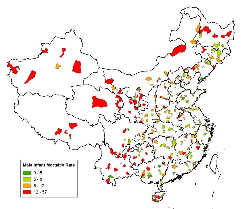
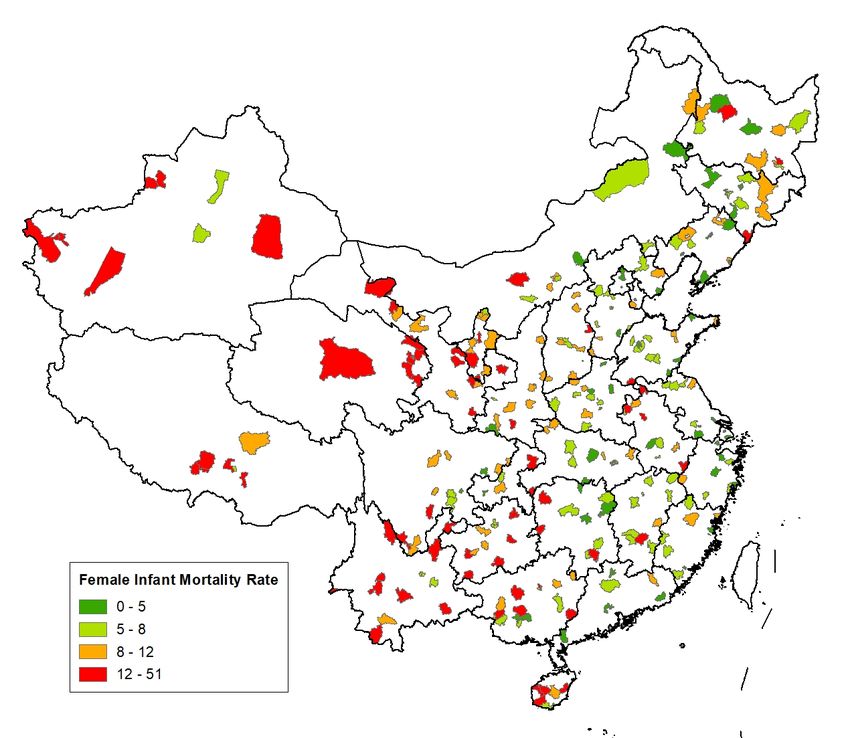
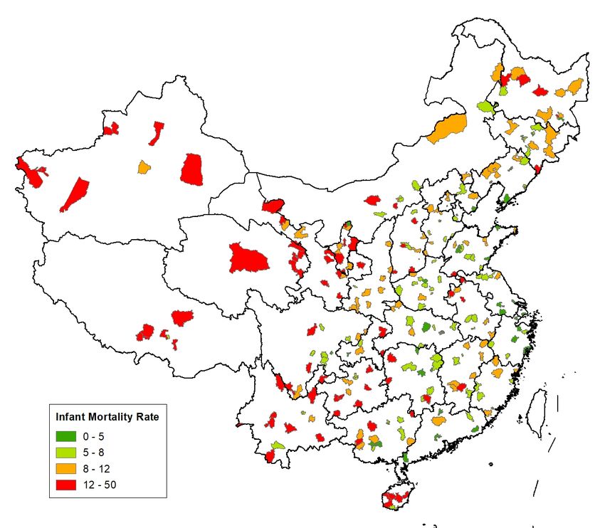
fungi, can cause pneumonia. For neonates, pneumonia is often acquired by aspiration (i.e.
aspiration pneumonia) after early rupture of membranes or during labor, or an initially
lower grade intrauterine infection associated with maternal chorioamnionitis. In other
words, pneumonia may develop in utero or in the first few hours of life, in contrast to other
forms of pneumonia occur later from a variety of established etiologic agents. As
contaminated water may affect the health status of mothers and impede the growth of fetus,
it may lead to higher neonatal mortality caused by pneumonia. At later stages of
development, the more-vulnerable infants are also more likely to get infected by bacteria
and viruses that cause pneumonia. Pneumonia is an important cause of infant death. In the
data, roughly 12% of infant deaths were caused by pneumonia.
 Congenital anomaly, also known as birth defects, is another major cause of infant
death. In the data, slightly more than 20% infant deaths are caused by congenital anomalies.
Congenital anomalies can be caused by single-gene defects, chromosomal disorders,
multifactorial inheritance, environmental teratogens and micronutrient deficiencies.
Contaminated drinking water is considered a major risk factor for congenital anomalies, as
it often carries toxins known for causing congenital disorders, such as heavy metals,
nitrates, nitrites, and fluoride.
 Low birth weight is a term used to describe babies who are born weighing less than
2,500 grams. Many factors can contribute to low birth weight, including the poor health
status of mothers, poor nutrition, alcohol and drug abuse, smoking, exposure to lead, air
pollution, and water pollution. Infant mortality due to low birth weight is usually directly
causal (e.g. Andrews, Brouillette, & Brouillette, 2008; Norton, 2005). In the data, almost
20% infant deaths are caused by low birth weight. Other causes of death account for 46%
of total deaths and are combined into a fourth category for empirical analysis.
 Table 1 presents the summary statistics of various mortality rates. The mortality
panel data (2009-2011) are collapsed to a 254 observation, location-level, and cross-
sectional data set. The average annual infant mortality rate is 8.0 per 1,000 live births.
Female infant mortality rate (7.5 per 1,000 live births) is lower than the male infant
mortality rate (8.5 per 1,000 live births). The infant mortality rate in rural areas is 8.8 per
1,000 live births while the number for cities is substantially lower: 6.3 per 1,000 live births.
The mortality rates for different causes are 0.86, 1.60, and 5.57 for pneumonia, low birth

 8

weight, and other causes respectively. It is worth noting that our sample means match the
official death rates recorded by the NMCHMS. Appendix Figures A1-A3 shows how infant
mortality rate varies by county and sex.

 Key Drinking Water Sources Data

Data for China’s key drinking water sources came from the Ministry of Water Resources.
These water sources are officially called “Centralized Drinking Water Sources in Cities
above the Prefecture Level” and are monitored directly by the central government. 3 The
data include 861 water sources, most of which are reservoirs and river sections with high
water quality. The geographical distribution of all the key drinking water sources is shown
in Figure 1.
 To be categorized as a key drinking water source, the water body has to meet a
series of technical standards, among which the high capability of providing a large amount
of unpolluted water is the most important. Typically, a key drinking water source should
be able to provide at least 20 million tons of unpolluted water annually. Water plants are
built near these water sources to produce purified water, which will then be delivered to
service areas through pipelines.
 The areas surrounding key drinking water sources are treated as the country’s
“protected area” and polluting activities are strictly prohibited. According to the
“Regulations on the Control of Pollution Prevention in Drinking Water Source Protection
Areas”: damaging the forests and plantations near the key water sources and dumping
industrial wastes, municipal wastes, manure, and other wastes into the waters are strictly
prohibited. 4 Ships and vehicles transporting toxic and hazardous substances are forbidden
to enter the protected areas. Pesticides and chemical fertilizers cannot be used, and even
fishing is not allowed in these areas.

 Surface Water Pollution Data

We collect surface water pollution data from China’s Environmental Statistical Yearbooks.

3
 This information can be accessed here: https://www.ynem.com.cn/uploads/soft/130107/12.doc.
4
 The regulations can be founded here:
http://www.mwr.gov.cn/zw/zcfg/bmgz/201707/t20170714_960211.html
 9

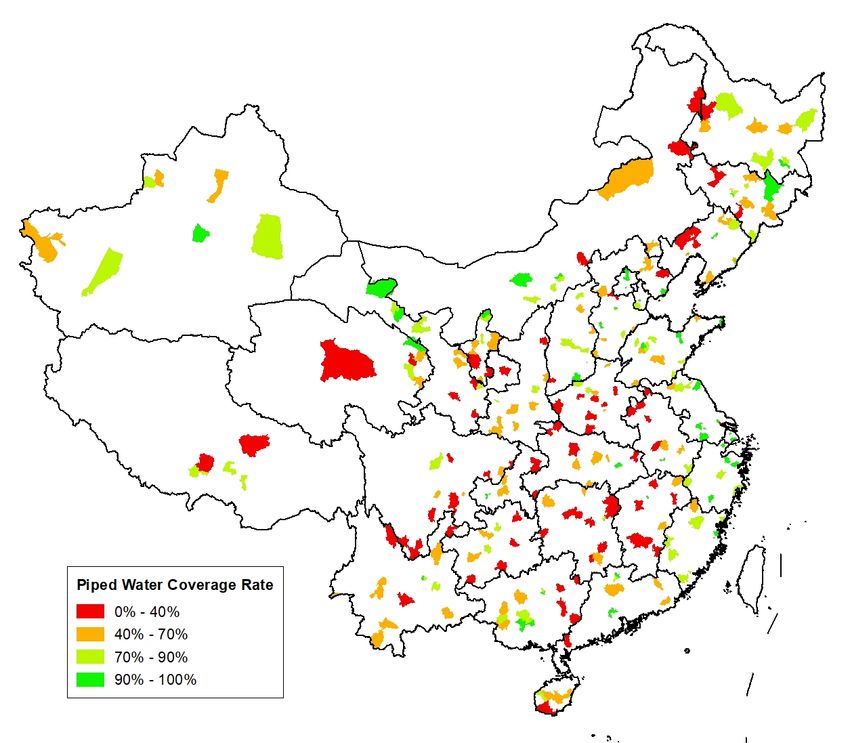
The water pollution data include 481 surface water quality monitoring stations; they record
surface water quality for major rivers, lakes, and reservoirs. The overall surface water
quality is graded using the concentrations of different chemical pollutant indicators
including the pH-value and the concentrations (measured by mg/L) of dissolved oxygen,
biochemical oxygen demand, ammonia, and nitrogen.
 The surface water quality is graded on a 6-degree scale, where Type I water is the
best quality water and Type VI is the worst. According to the China Ministry of Water
Resources, Type I water is an “Excellent” source of potable water. Type II water is a
“Good” source of potable water. Type III water is “Fair.” Pathogenic bacteria and parasites
ova can sometimes be found in Type II and III water so drinking it will introduce pathogens
into human consumers. Thus, Types II and III water should be purified and treated (such
as by boiling) before drinking. Type IV water is polluted and unsafe to drink without
advanced treatment, which is only possible at water supply plants. Type V is seriously
polluted and can never be used for human consumption. Type VI water is called “Worse
than Type V Water,” and any direct contact with it is harmful to humans. We use number
1-6 to represent different water quality grades with 1 being the cleanest and 6 being the
dirtiest.
 Appendix Figure A4 shows the geographical distribution of the stations and the
pollution levels. The pollution map shows that northern China is more polluted than in
southern China. According to our data, the average water quality level in north China is
3.7 compared with 2.5 in the south. Approximately 36 percent of China’s surface water is
severely polluted (IV, V and VI) in 2010.

 Piped Water Coverage and Control Variables

We collect piped water coverage data from China’s 2010 Census. The data were gathered
by asking households whether there was piped water in their houses. The piped water
coverage in a county is defined as the share of households that have piped water in their
houses. The piped water coverage rates at the NMCHMS locations are shown in Appendix
Figure A5.
 We assemble a rich set of control variables that are particularly relevant to infant
health at the county level. These variables include per capita income, fiscal expenditure per

 10

capita, fiscal expenditure on healthcare per capita, fiscal expenditure on maternal and child
healthcare per capita, number of maternal and child hospitals per 100,000 people, and the
number of maternal and child healthcare professionals per 100,000 people. We also collect
the share of population working in the manufacturing from the 2010 Census as a control
variable.
 After matching the mortality data with control variables, the full sample includes
254 infant mortality surveillance areas. The average piped water coverage rate is 69%.
Almost 14% of the Chinese population are employed in the manufacturing sector. Average
income, fiscal expenditure per capita, healthcare expenditure per capita, and maternal and
child healthcare expenditure per capita are approximately 11,000, 38,000 and 6,700, and
1,300 Yuan in 2010. There are on average 0.34 hospitals and 28 professionals specializing
in maternal and child health care per 100,000 people.

 IV. Empirical Strategy

 Econometric Model

We start with an Ordinary Least Squares (OLS) regression model:
 = 0 + 1 + ′ + + (1)
where and are the infant mortality rate and the piped water coverage rate in
county i of province j, is a set of county-level variables that may affect infant mortality,
 are province fixed effects, and is the error term.
 Our objective is to identify the average effect of accessing piped water on infant
mortality in NMCHMS locations. The parameter of interest in the model is 1 . The
identifying assumption for 1 to capture the unbiased effect is that the error term is
uncorrelated with piped water coverage, conditional on the control variables:
 � � , � = 0. In other words, we have to control for all the determinants of
infant mortality that are related to piped water coverage. This assumption is of course
overly strong because many confounding factors are not observable to the researchers. The
areas that have a higher rate of piped water coverage may have some unspecified
characteristics that differ from the areas with a low coverage rate; and these differences

 11

may be correlated with infant mortality. If the unobserved confounders (such as family
wealth) are positively correlated with piped water coverage and infant mortality, OLS
estimates will over-estimate the effects. Conversely, if the unobserved confounders are
negatively correlated with piped water coverage and infant mortality, the OLS estimates
will be biased downward. In the Chinese context, many of the central government’s public
health campaigns (such as providing subsidies for hospital delivery) often target less-
developed areas; this sometimes makes the relatively poor areas better supplied with health
resources than the slightly richer areas. When this happens, the OLS estimates may
underestimate the true health effect of piped water coverage.
 We address the problem of endogeneity by using an instrumental variable approach.
We use the least cost distance as the instrumental variable for piped water coverage and
estimate the following two-stage equations:
 = 0 + 1 + ′ + + (2)
 � + ′ + + 
 = 0 + 1 (3)
where is the least-cost distance between an NMCHMS location and its least costly
major water source (e.g. a reservoir); and are similarly defined as in equation (1).
 In the first stage, equation (2) estimates the effect of the least-cost distance on piped
 � , is used
water coverage. The predicted piped water coverage rate from equation (2), 
in the second stage, equation (3), to estimate the impact of piped water coverage on infant
mortality. The error terms, and , might be correlated across space. For example, child
health programs provided by the provincial government apply to all cities and counties in
the province. To avoid potential biases in the estimation of the standard errors, we allow
for an arbitrary covariance structure. In both equations, the province fixed effects are
included to reflect the fact that the piped water infrastructure is usually constructed within
the same province.
 The identification strategy can be further augmented if the data have a panel
structure. Specifically, one can use the least cost distance to instrument the changes in
piped water coverage over time for different locations. This would be the ideal situation if
the piped water coverage data could be traced back decades ago, when all the places had
no piped water connection. But unfortunately, we can only find piped water data in China’s
2000 and 2010 population census. In 2000, many cities with low costs of piped water
 12

connection had already have high levels of coverage, making the least cost distance
instrument to be negatively, rather than positively, associated with the changes in piped
water coverage between 2000 and 2010. While strengthening the identification along this
dimension is infeasible in this study, we hope future research can explore this arguably
stronger identification strategy.

 Instrumental Variable

Given the data limitation, we rely on cross-sectional variation to estimate the health impact
of piped water coverage. As discussed, construction of the piped water system depends
heavily on the distance and terrain between a major drinking water source and a service
destination. It is more expensive to build piped water infrastructure if a county is farther
away from the water source, and costlier still if the terrain is rugged.
 Consequently, we calculate the cost distances between the focal counties and the
water sources and use the least-cost distance between a focal county and its nearby water
sources as an instrument for piped water provision in the county. Cost distance is one of
the distance metrics that account for the topological features of the terrain. 5 It captures the
salient feature that there is a cost or impedance associated with moving a unit distance over
any location, and this cost is determined not only by distance but also by specific terrain
features.
 To construct the cost distance measure, we first geo-code all the key drinking water
sources and NMCHMS locations. Then we construct a cost surface over China using
ArcGIS. The cost surface is constructed using a digital elevation model (DEM); we assign
a higher cost value for a steeper slope and a more rugged area. We also incorporate a
detailed waterway network in the calculation. The waterways along the key water sources
are relevant because they may carry similar high-quality natural water, which can be used
to provide clean piped water. It is thus cheaper for a county that is closer to waterways to
transport water. The least-cost distance thus reflects the slope, the terrain, and the river
factors from each water source to each NMCHMS location. The least-cost path is then

5
 Other ways to measure the distance between two points include the Euclidean distance (an unconstrained
straight line), Geodesic distance (when travel is constrained to the surface of a sphere), and network distance
(when travel is constrained to a linear network).
 13

chosen from all the source-to-county cost paths and the associated cost distance is extracted
from the least-cost path. In Appendix I, we describe the steps of constructing the cost
surface and least-cost paths. The process requires specifying some parameters based on the
researcher’s judgment, including assigning cost estimates to different elevation scenarios
and incorporating extra considerations (such as river flows) in the cost calculation. We use
the default parameters proposed by engineering studies for constructing the cost surface.
Then we check the robustness of our findings using alternative ways to estimate the least-
cost distance. The details of alternative cost distance measures are elaborated in the
robustness check section.
 Figure 2 illustrates the constructed least-cost paths between the key water sources
and different counties. The identification relies on the assumption that the least cost
distance affects the infant mortality only through its impact on piped water coverage:
 � , � = 0 and � , � ≠ 0 . Because the instrument is constructed
purely based on cost considerations, it should be uncorrelated with most unobserved
demand-side determinants of infant mortality, such as wealth and household health inputs.
We expect the least-cost distance to be negatively correlated with piped water coverage
because building piped water infrastructure is more expensive for counties remote from
major drinking water sources.

 V. Results and Implications

 Validity of the Instrumental Variable

We first discuss the validity of the instrumental variable. The first requirement of a valid
instrument is its power in predicting the endogenous variable. Appendix Table A1 reports
the results from estimating equation (2). We find that the least cost distance is statistically
significant at the 1% level and the F-statistics exceed the conventional criteria for a
powerful first stage in all models (Stock & Yogo, 2005). Partial R-Squared (average=0.29)
also confirms that the instrument is a strong predictor of piped water coverage.
 The second requirement for a valid IV is that the IV should affect the outcome only
through its impact on the endogenous variable, i.e. the IV is excludable from the second-

 14

stage regression. While this requirement cannot be credibly tested, we provide two sets of
results that suggest that the least-cost distance IV is likely exogenous. First, the estimated
coefficients of the IV in Table A1 are remarkably robust to the inclusion of different control
variables, such as income and government spending on health care. These control variables
are often recoganized as important determinants of local infant health, but they have little
impact on the first-stage regression results. This finding suggests that the IV is orthogonal
to local socio-economic and public health conditions. Second, we directly regress the least-
cost distance on the set of control variables. Table 2 reports the results. No significant
correlations between the IV and control variables are detected in the regressions, except
the mountain area dummy. The mountain area dummy is expected to be correlated with the
cost distance because it is more costly to build piped water infrastructure in mountainous
regions. To address this concern, in all the regressions, we include mountain dummies as a
control, which helps capture the fundamental difference in water consumption habits
between the mountainous and plain areas. 6 In essence, we are comparing mountainous
locations (or plain locations) that are closer to drinking water sources with mountainous
locations (or plain locations) that are further away from the water sources measured by cost
distances.

 Main Results

We present the main estimation results in Table 3. For all models, we use the total
population as the sampling weights. In Panel A, the dependent variable is the logarithm of
infant mortality rate per 1,000 live births. In Column (1), we find that a 10-percentage-
point increase in county-level piped water coverage will lead to a 17% decrease in infant
mortality when no control variable is included. Column (2) adds per capita income to
control for the resource differences across different counties. In Columns (3) to (6),
additional control variables are introduced into the regressions. Column (3) adds a surface
water (lakes and rivers) quality variable to control for potential differences in infant

6
 People living in mountainous areas often use spring water for consumption, while those living in plain areas
often fetch water from the well for consumption. However, the results remain similar if we do not control for
mountain area fixed effects in our regressions.
 15

mortality due to the pollution level in local surface water body. 7 Column (4) adds two
variables of government expenditures: fiscal expenditures per capita and fiscal
expenditures on healthcare per capita. These measures government’s inputs in social
welfare and public health. Column (5) adds resources devoted to maternal and child care
including government child healthcare expenditures per capita, the number of maternal and
child care hospitals per 100,000 people, and the number of maternal and child care
professionals per 100,000 people. Column (6) adds an indicator for rural areas to capture
and rural-urban disparities, the share of employment in manufacturing to control for the
structural difference in the local economy across different counties, and an indicator for
mountain area to caputure the differences between mountainous areas and plain. 8 Column
(7) includes all the available controls and shows that a 10-percentage-point increase in
piped water coverage will reduce the infant mortality rate by 16%. The estimated
coefficients are remarkably stable across different models and all of them are statistically
significant at the 1% level.
 Panel B reports the results using infant mortality rate without log-transformation as
the dependent variable. The model specifications are the same as those in Panel A. If we
compare the results of Column (1) through (7), we also see that including control variables
does not significantly alter the estimates. A 10-percentage-point increase in piped water
coverage is estimated to reduce the infant mortality rate by 1.179 per l,000 live births when
all variables are controlled in Column (7). This translates into a 15% reduction of infant
mortality relative to the mean. These estimates are quantitatively similar to those in Panel
A. The consistency of estimates across alternative forms of the outcome variables shows
that our results are not influenced by outliers or the distribution of the outcome variable.
 Column (8) reports the OLS estimates. Compared with the IV estimates, we find
that the OLS estimates are smaller: expanding piped water coverage by 10% is associated

7
 Surface water quality could affect infant quality directly and indirectly. Direct influence involves
consumption of pollution water by infants or their mothers. Indirect influence is often through food chains.
For example, vegetables and meat products could be contaminated by pollutants in surface water.
8
 Table 2 shows that the instrument is predictive of a mountainous region, which may also make it more
difficult for families to seek care. Other than using a mountainous region dummy as a control, we also used
two more terrain variables with finer variations than the mountain dummy. One is average land slope of the
county or district, the other is terrain ruggedness index which meansures elevation difference between
adjacent cells of a digital elevation grid in a county or city district. The results are very similar to those in
Table 3 and are available upon request.
 16

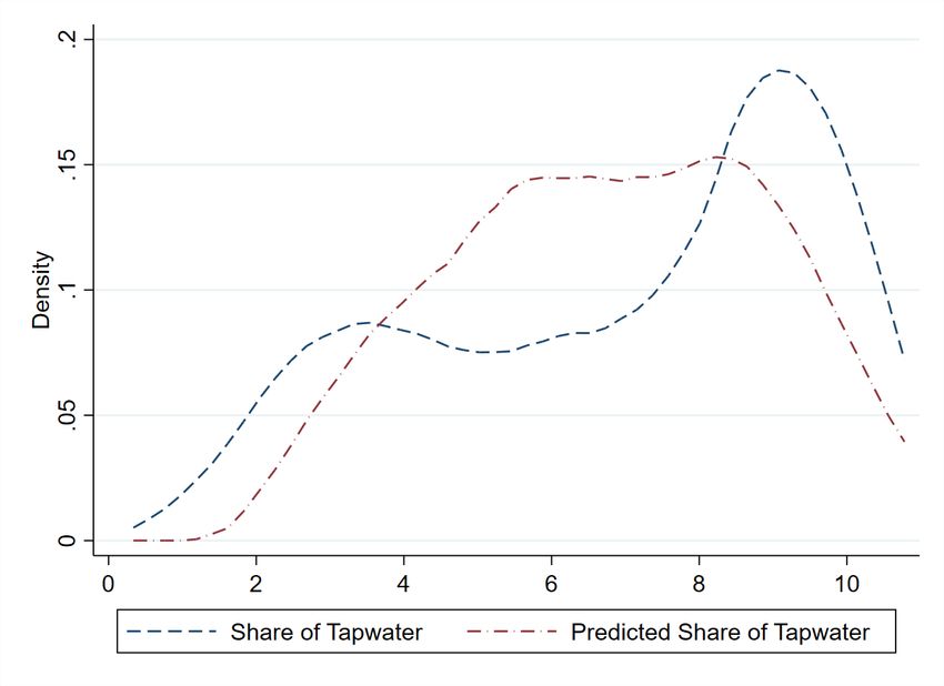
with an 8.6% decrease in infant mortality rate. The IV estimates are almost twice as large
as OLS estimates. The difference is unlikely due to the fact that the IV approach estimates
the local average treatment effect because the IV variation is at similar levels of the overall
variation of piped water coverage. 9 Instead, this is likely due to the endogeneity of the
piped water provision. Failure to account for this endogeneity significantly underestimates
the effect of piped water on infant health.

 Results by Sex, Development Stage, and Cause of Death

We investigate how the impact of clean drinking water varies across sex, development
stage, and causes of death. Estimating the impact for males and females separately could
potentially allow us to examine whether clean drinking water contributes to the difference
in male and female infant mortality rates. Table 4 presents estimation results. Columns (1)
to (4) separately estimate the effect of piped water access for males and females. The
provision of piped water decreases both male and female infant mortality rates. With all
the control variables are included, a 10-percentage-point increase in piped water coverage
leads to a 16% reduction in male infant mortality rate and a 15% decrease in female infant
mortality rate. Therefore, there is no significant impact heterogeneity across sex because
the two estimates are not statistically different from each other. The results contradicts the
predictions of the fragile male literature (Kraemer, 2000). We suspect the son prefence in
China (e.g., Das Gupta et al., 2003) provides more protection and care to male infants than
female infants and offsets the male disadvantages at birth (e.g. the biological fragility of
the male fetus).
 To understand the importance of clean water in different stages of infant
development, we estimate the effects of piped water coverage on neonatal and post-
neonatal mortality rates. Columns (5) to (8) report the results. For neonatal mortality, a 10-
percentage-point increase in piped water coverage reduces the mortality rate by 13%. For
post-neonatal mortality, it reduces the mortality rate by 17%. The difference in two

9
 To assess this, we computed the predicted values of piped water coverage when the least cost distance
increases or decreases by one standard deviation (SD) from the mean, based on estimating equation (2). The
adjusted mean for a one SD decrease in least cost distance is 0.551 and a one SD increase is 0.763. The
unadjusted mean of piped water coverage rate is 0.667, which is bounded by the two adjusted means. Figure
A6 shows significant overlaps between real share of piped water and the predicted values using the instrument.
 17

estimates is not statically significant suggesting clean water is important throughout the
early development of an infant.
 We also examine the causes of death, which is a relatively neglected topic in the
literature, to provide a further understanding of how diseases related to water conditions
affect infant mortality. Table 5 presents the estimates. Columns (1)-(2) show results for
deaths caused by pneumonia. Access to piped water significantly reduces infant mortality
caused by pneumonia. Expanding piped water coverage by 10 percentage points decreases
mortality rate by 13%. For deaths due to low birth weight, in Columns (3)–(4), we find the
effect is also significant although a little smaller in magnitude: a 10 percentage points
increase in piped water coverage decreases infant mortality rate by 11%. For all other
causes, in Columns (5)–(6), we estimate that a 10-percentage-point increase in piped water
coverage reduces the mortality rate by 11%. The results suggest that water quality has
pervasive influences on infant health.

 Mortality of Children Aged 1-5

To evaluate the impact of piped water on young children, we extend our analysis to the
mortality rate of children older than 1 year and younger than 5 years of age (hereafter,
under-5 mortality). Compared with infants, young children have more matured immune
systems and are less susceptible to environmental risks than infants are. We construct a
dependent variable as the ratio of the number of deaths of children aged 1-5 to the total
number of children alive in the same age group. 10 Appendix Table A2 presents the
summary statistics of various mortality rates for children aged 1-5.
 Table 6 reports the results. We find that none of the coefficients is statistically
significant, and more importantly, the magnitude of the coefficients is close to zero. While
the null-effect for children is consistent with several previous studies (e.g., Gamper-
Rabindran, Khan, & Timmins, 2010; Rutstein, 2000), we want to caution readers that we
are not claiming piped water has no benefits on children aged 1-5. It could be possible that
we do not have enough power to detect its impact on children because the mortality rate
for this group is very low.

10
 The number of children aged 1-5 years is from China’s 2010 Census.
 18

Robustness Checks

We check the robustness of our main findings in several ways. First, we investigate whether
our results are confounded by migration. Historically, Chinese people were restricted to
live in one’s birthplace under the Hukou (household registration) system. Because of the
opening and reform policies since the early 1980s, migration becomes much more common
and many people move away from their birthplaces for school or work. This creates
challenges for our analysis because some individuals might migrate in response to local
environmental risks. For example, if wealthy people choose to migrate from areas without
piped water to areas with piped water and they have more resources to take care of the
pregnant women and infants, then we will overestimate the impact of piped water on infant
mortality. Our data do not allow us to identify the exact reason why people migrate and the
percentage of infants born to migrant parents, but excluding locations with high migration
rate could to some extent alleviate this concern. Using individual data from the 2005
Census, we define a migrant as a respondent who lives in a region that differs from his/her
origin Hukou region. We then calculate the share of migrants for the 254 NMCHMS
locations in our analysis. We exclude the locations where migrants account for more than
15% of the population and re-estimate the models. The results presented in Panel A of
Table 7. We find that the estimated effects are greater than, but qualitatively consistent
with those in Tables 3-5 after the high-migration regions are excluded. Consequently, we
conclude that our estimates are lower bounds of the true effect of clean water on infant
mortality.
 Second, a quarter of the monitored NMCHMS locations are in minority areas.11
The piped water coverage rate in minority NMCHMS locations is on average 10 percent
lower than that in non-minority locations. Birth attending and family child care practices
in China are known to vary by ethnic groups, which might affect the patterns in infant
mortality. To check whether our findings are driven by the minority groups, we restrict the
sample to non-minority NMCHMS locations and present the results in Panel B of Table 7.
The estimated coefficients are similar to the main results in Tables 3-5. This indicates that

11
 Those minority areas are either designated as a minority autonomous region or locations with more than
50% minority population.
 19

the cultural differences in birth/child caring traditions are not affecting our results.
 Third, we check the results without the mountain area control. The mountain area
dummy is the only variable is that is strongly correlated with our instrument. While this is
well expected, one may be concerned that it threatens the validity of the instrument. As a
robustness check, we exclude the mountain area dummy in the regressions and replicate
the main findings in Appendix Table A3. We find that the estimates remain quantitatively
similar to those in Tables 3-5. These findings suggest that the mountain area dummy
variable, while being correlated with the lease cost distance variable, only affects the tap
water coverage through the least cost distance channel.
 Fourth, a large number of studies show that air pollution has negative health
impacts on infant health (Chay & Greenstone, 2003b; Currie & Neidell, 2005; Luechinger,
2014). We collected air pollution data including PM10 and SO2 for 386 sites across China
and assigned the air pollution levels to NMCHMS locations using similar rules as we assign
water pollution levels to NMCHMS locations. 12 We include both PM10 and SO2 as control
variables and re-estimated Table 3. The results are presented in Appendix Table A4. We
find that the coefficients of piped water coverage are almost identical to those in Table 3.
This indicates that clean water access affects infant mortality through mechanisms different
from air pollution.
 Finally, we provide the reduced-form results to show how the least-cost distance
affects the infant mortality rate and under-5 mortality rate in Appendix Table A5. Results
show that a 1-percent increase in the least cost distance is estimated to increase infant
mortality by 0.16 percent. The effect is statistically significant across gender and for
different causes of deaths. These results are consistent with our design of the instrumental
variable that regions with easier access to clean water sources are more likely to use clean
water and have a lower infant mortality rate. In contrast, we reject the null hypothesis that
the least cost distance is statistically significantly associated with the under-5 mortality rate
in all models. In other words, the least cost distance does not affect the mortality rate of
older children as much as infants.

12
 The only difference between the two matching rules is the tolerance distance. We assigned missing air
pollution values for an NMCHMS location if there is no air monitor sites within 150 km radius. We examined
the sensitivity of the results to alternations thresholds and find similar results. Note that multi-city PM2.5 data
were not available in China until 2013.
 20

VI. Heterogeneity: Surface Water Pollution and Rural vs. Urban

The impact of piped water provision may vary across different NMCHMS locations. In
this section, we explore two important heterogeneities. First, we explore the difference in
surface water pollution in different regions. Second, we examine the possibility that the
impact of piped water may matter more in rural areas where the piped water coverage rate
is low.

 Surface Water Pollution Level

The impacts of clean drinking water are complicated by the fact that individuals may adjust
their exposure in response to water pollution. This concern is particularly relevant because
individuals in the most polluted regions have the strongest incentive to adopt avoidance
behavior. If individuals compensate for higher water pollution by reducing exposure,
estimates that do not account for these responses will understate the full welfare effects of
clean water access. Therefore, the relationship between surface water pollution and health
is difficult to identify because people take avoidance behavior. To shed light on these issues,
in this section, we separately examine the impact of piped water provision in slightly
polluted and severely polluted regions.
 To assign a water pollution level to each NMCHMS location, we take two steps.
First, we calculate the distance between each of these water pollution monitoring stations
and NMCHMS locations. The distance between each of these 881 stations and the 254
NMCHMS locations yielded a full matrix of 254 × 481 calculated distances. 13 Second, our
measure of water pollution for an NMCHMS location was calculated as follows: if an
NMCHMS location was within 25 kilometers of a valid station reading, the nearest station's
reading was used. If an NMCHMS location was not within 100 kilometers of any of the
stations, the NMCHMS location was excluded from the sample. 14 This resulted in the
exclusion of 44 NMCHMS locations. If an NMCHMS location was within 100 kilometers

13
 The coordinates of the county capital, the centroid of the city district of the IMR sites, and the coordinates
of monitor stations were used to calculate an exact distance between the two.
14
 We also examine the sensitivity of the results to alternations threshold for the cases where we only use the
nearest monitor (rather than a weighted average). The analysis in the paper assigns water pollution level
based only on the nearest station when the nearest station is within 25 km of the NMCHMS location and uses
weighted averages across stations in cases where the nearest station is further than 25 km but less than 100
km away.
 21

of a station but not within 25 kilometers, the pollution was calculated as the weighted
average of water pollution at each station with a valid reading within 100 kilometers, with
the weights determined by the inverse of the distance between the two points. 15 If a station
had no valid water pollution reading for 2010, it was assigned a zero weight and did not
enter into the calculation. Figure 3 shows the water quality levels of 254 NMCHMS
locations after the matching process.
 Table 8 reports the IV estimation results. The outcome variables include overall
infant mortality rate, male and female infant mortality rates, and mortality rates for
different causes. We split the sample based on the surface water pollution level. Panel A
includes areas with slight water pollution (water quality is less than or equal to grade 3)
and Panel B includes areas with high water pollution levels (water quality is greater than
grade 3). The results show that piped water provision has highly heterogeneous health
impacts with respect to local surface water pollution levels. A 10-percentage-point increase
in piped water coverage can reduce the infant mortality rate by 21% for the slightly polluted
regions and the estimate is statistically significant. In contrast, the estimated effect for more
polluted regions is much smaller in magnitude and statistically insignificant. The same
pattern can also be found for gender-specific and most disease-specific mortality rates. 16
 There are two possible explanations for the heterogneous impacts of piped water
coverage with respect to local surface water pollution levels. The first explanation is that
surface water quality might be somehow correlated to the point-of-use quality of piped
water, which consequently lead to the heterogenous impacts between the two groups of
places. However, this is highly unlikely becasue all the drinking water sources (used for
piped water) have to meet the national water quality standards and the variations in water
quality across different sources are small (Type I and Type II water quality). In addition,
source water has to be treated in water plants to further ensure that it meets the drinking
water standards. Bacterias, water pollutants, and other toxic chemicals have to be

15
 The results are robust to different choices for the functional form. This is discussed further in Part 3.
16
 The only exception is congenital anomalies. We find that providing clean drinking water can also decrease
congenital anomalies in severely polluted areas. One likely explanation to this irregularity is that surface
water pollution can affect birth defects through other indirect channels, such as food intake and
biomagnification. In severely-polluted regions, stop drinking polluted water is able to immediately reduce
acute diseases caused by water contamination (i.e. the “low-hanging” fruits), but it alone is not sufficient to
mitigate the accumulative health impact because people are still exposed to a heavily-polluted environment.
 22

removed before the water is delivered to different households, making piped water
quality more homogeneous across different locations than surface water.
 The second explanation for this phenomenon is that if rivers and lakes become
severely polluted and the pollution becomes visible, people will stop consuming their
waters. 17 To verify this conjecture, we examine Chinese people’s water-drinking patterns
using data from China Health and Nutrition Survey (CHNS). 18 The CHNS data provide
province and rural/urban information to researchers, so our analysis is at the province
level. We use data from the 2009 wave and assign a water pollution grade to each
province by averaging the pollution readings of all water monitor stations in the same
province. 19 There are two types of households: those having access to piped water in their
yards (not necessarily in their houses) and those without access to piped water (who need
to obtain drinking water from groundwater, open well, creek, spring, river, lake, and
ice/snow). The CHNS survey asks each respondent: "Do you normally drink bottled
water?" Then we compare the bottled water consumption between more polluted and less
polluted provinces, based on the provincial water pollution level. Table 9 reports the
results. Among rural respondents who have no direct access to piped water, only 58% of
them drink bottled water in the slightly polluted areas; in sharp contrast, over 95% of
rural residents do so in the heavily polluted areas. Such a difference is much smaller
when piped water is available. The evidence is consistent with our conjecture that people
adopt avoidance behavior to mitigate the impact of water pollution. As a result, the
estimated impact of clean water in heavily polluted areas is downward biased by people’s
avoidance behavior.

 Rural vs. Urban

More than half of China’s population (including people in towns) still live in rural areas.

17
 Using China’s 2000 Census data, He and Perloff (2016) found that the relationship between surface water
pollution and infant mortality was non-monotonic: slightly polluted surface water was the most dangerous in
China. They attributed the phenomenon to people’s avoidance behavior when water quality is very low.
18
 The CHNS is a longitudinal individual and household survey began in 1989 with the goal of understanding
how social, economic, and demographic changes in China affected nutrition and health-related outcomes
across the life cycle. The sample began with eight provinces in 1989 and currently covers 7,200 households
with over 30,000 individuals in 15 provinces. The relevant survey questions are presented in Appendix II.
The CHNS datasets and more details can be accessed at https://www.cpc.unc.edu/projects/china.
19
 . We only use the 2009 wave because the water pollution data are available for 2009.
 23