The movements of Alpine glaciers throughout the last 10,000 years as sensitive proxies of temperature and climate changes
←
→
Page content transcription
If your browser does not render page correctly, please read the page content below
EPJ Web of Conferences 232, 02002 (2020)                                                            https://doi.org/10.1051/epjconf/202023202002
HIAS 2019

       The movements of Alpine glaciers throughout the last 10,000 years as sensitive
       proxies of temperature and climate changes
       Walter Kutschera1,*, Gernot Patzelt2, Joerg M. Schaefer3, Christian Schlüchter4, Peter Steier1, and Eva Maria Wild1
       1
         VERA Laboratory, Faculty of Physics, University of Vienna, A-1090 Vienna, Austria
       2
         Gernot Patzelt, Patscher Strasse 20, A-6080 Innsbruck-Igls, Austria
       3
         Joerg M. Schaefer, Geochemistry, Lamont-Doherty Earth Observatory, Pallisades, NY 10964-8000, USA
       4
         Christian Schlüchter, Institute of Geological Sciences, University of Bern, CH-3012 Bern, Switzerland

                    Abstract
                    A brief review of the movements of Alpine glaciers throughout the Holocene in the Northern Hemisphere (European
                    Alps) and in the Southern Hemisphere (New Zealand Southern Alps) is presented. It is mainly based on glacier studies
                    where 14C dating, dendrochronology and surface exposure dating with cosmogenic isotopes is used to establish the
                    chronology of advances and retreats of glaciers. An attempt is made to draw some general conclusions on the
                    temperature and climate differences between the Northern and Southern Hemisphere.

      1 Introduction                                                         radiocarbon dating, surface exposure dating of rocks and
                                                                             moraines with various cosmogenic radionuclides (10Be,
      It is well known that the Holocene, i.e. the geological time           14
                                                                                C, 26Al, 36Cl), and geomorphological considerations [10-
      period following the end of the Last Ice Age, enjoyed                  22].
      relatively stable temperatures. But glaciers are sensitive                 The atmospheric CO2 concentration was remarkably
      proxies to even small temperature and/or climate changes.              constant during the last 10,000 years, changing by only 20
      Thus, the globally observed retreat of Alpine glaciers and             ppm [1]. Such small CO2 variations are unlikely to trigger
      polar ices sheets since about 1850 AD (the end of the so-              the observed glacier movements. It is therefore possible
      called Little Ice Age and interrupted by three re-advances)            that small solar activity variations [23], enhanced by
      has been linked to the temperature increase caused by                  (hitherto largely unknown) feed-back processes on Earth
      human activities, particularly due to the continuous                   caused the observed glacial fluctuations [24]. Whatever
      increase of the CO2 concentration in the atmosphere [1]. It            the cause of these natural fluctuations, they constitute a
      is interesting to note that a change in the surface                    “background” which is now being modified in a complex
      temperature on Earth with increasing CO2 concentration in              way by human activities. The challenge is then to evaluate
      the atmosphere was already discussed more than 100 years               the human signal correctly, and try to make predictions
      ago by the Swedish chemist and Nobel Laureate Svante                   about the climate in the near future [25]. There is an
      Arrhenius [2]. Discussions are ongoing now to define a                 ongoing discussion about the certainties and uncertainties
      new geological period called “Anthropocene” [3, 4],                    of these predictions [e.g. 26]. In spite of great efforts
      where man’s influence on the environment is significant                around the world to reduce anthropogenic CO2 emissions,
      and distinct [5, 6]. Even though the global retreat of                 it appears doubtful whether this is currently more than a
      glaciers since 1850 is considered to be a fingerprint of               “pious wish” [27].
      man’s influence on the climate, it is now evident that                     The current work cannot give an answer to these
      considerable glacial fluctuations occurred already much                important questions. Rather it will present evidence for the
      earlier during the Holocene, when human impact was                     waxing and waning of Alpine glaciers in both the Northern
      negligible.                                                            and Southern Hemispheres throughout the Holocene. An
           In a way, the interest in Alpine glaciers of the past             attempt will be made to explain at least some of these
      started with the accidental discovery of the famous Iceman             fluctuations from first principles. Even though the
      Ötzi in 1991, a naturally mummified body which was well                complexity of the climate may only allow crude estimates
      preserved for 5200 years in the icy environment of a high              of those principles, we simply follow the advice of the late
      mountain pass (3210 m a.s.l.) in the Ötztal Alps [7-9].                Murray Gell-Man: “Nature is most easily described by a
      Since then, several forward and backward movements of                  sequence of approximations,” [28].
      glaciers in the European Alps and in the New Zealand
      Southern Alps throughout the last 10,000 years have been
      established with the help of dendrochronology,
       ______________________________
       *
         email: walter.kutschera@univie.ac.at
© The Authors, published by EDP Sciences. This is an open access article distributed under the terms of the Creative Commons Attribution License 4.0
(http://creativecommons.org/licenses/by/4.0/).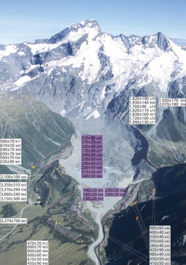
EPJ Web of Conferences 232, 02002 (2020)                                                           https://doi.org/10.1051/epjconf/202023202002
HIAS 2019

     2 Paleorecord of Temperature and CO2                                   currently goes back 800,000 years [29, 30], and shows the
                                                                            well-known Milankovic cycles of the ice ages first
     The records of temperature and atmospheric CO2                         discovered in the δ18O record of foraminifera in deep-sea
     concentration on Earth show considerable variation over                sediment cores [31]. Efforts to drill ice cores in Antarctica
     the last 500 million years (Fig. 1). In particular, the CO2            back to 1.5 million years are under way [32, 33]. Except
     concentration during the time of the dinosaurs (~240 – 65              for the brief interglacial periods, the CO2 concentration
     million years ago) was around 1000 ppm, and the mean                   stays at its lowest value in this period and reaches about
     temperature about 6 oC warmer than today. From Fig. 1,                 200 ppm at the glacial maximum 20,000 years ago. After
     one can see that during the last 10 million years, a gradual           warming up to the Holocene some 10,000 years ago, both
     lowering of the temperature and of the CO2 concentration               relatively stable temperature and CO2 concentrations
     occurred.                                                              persist. The rapid increase of CO2 during the last 60 years
           Around 2.5 million years ago (beginning of the                   from about 300 ppm to currently 415 ppm is well
     Pleistocene), major glaciations in both Antarctica and                 documented [1].
     Greenland set in. The record of ice cores from Antarctica

                                                     Temperature of Planet Earth
                                              https://en.wikipedia.org/wiki/File:All_palaeotemps.png
        ∆T                                                                                                                               ∆T
       (oC)                                                                                                                              (oC)
       +14                                                                                                                               +14
       +12                                                                                                                               +12
       +10                                                                                                                               +10
        +8                                                                                                                                 +8
        +6                                                                                                                                 +6
        +4                                                                                                                    2100         +4
        +2                                                                                                                    2050         +2
          0                                                                                                                                 0
         -2                                                                                                                                -2
         -4                                                                                                                                -4
         -6                                                                                                                                -6
              500 400 300 200 100 60 50 40 30 20 10 5             4     3     2    1   800 600 400 200 20       15    10     5       1
                                          Years before present (Myr)                           Years before present (kyr)
       CO2                                                                                                                            CO2
      (ppm)                                                                                                                          (ppm)
      5,000                                                                                                                              5,000
                                              Atmospheric CO2 concentration of Planet Earth
                                                           Foster et al., Nature Comm. 8:14845 (2017)
      2,000                                                                                                                              2,000

      1,000                                                                                                                              1,000

        500                                                                                                                               500

        200                                                                                                                               200

        100                                                                                                                               100

              500 400 300 200 100 60 50 40 30 20 10 5             4     3     2    1   800 600 400 200 20       15    10     5       1

     Figure 1. Summary of temperature and CO2 concentrations on Earth for the last 500 million years. The figure is a composite from the
     original temperature record [34] and the CO2 record [35]. The CO2 record was adjusted to the same time scale as the temperature record.
     Possible temperature increase in 2050 and 2100, respectively, predicted by some climate models are indicated with red dots on the
     rightmost temperature axis.

     3 Movement of Alpine glaciers during                                   evolved into a new field sometimes called “glacial
     the Holocene                                                           archaeology”. Besides the archaeological aspect in the
                                                                            study of glaciers, there is the sensitivity to small climate
     The accidental discovery of the Iceman “Ötzi” in 1991 [7-              changes which became apparent through multiple periods
     9], and the appearance of human artefacts and natural                  of forward and backward movements of glaciers
     materials released from receding Alpine glaciers [22],                 throughout the Holocene [11].

                                                                       2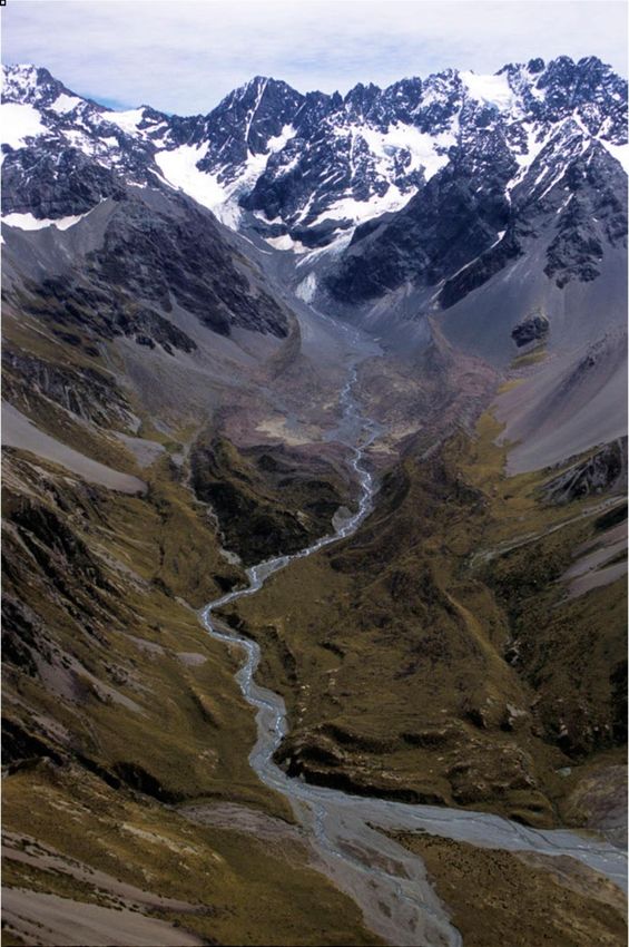
EPJ Web of Conferences 232, 02002 (2020)                                                                      https://doi.org/10.1051/epjconf/202023202002
HIAS 2019

     3.1 The European Alps                                                              3.1.1 The Pasterze glacier

     Glacier movements of the past have been studied in many                            The rapidly receding glaciers in our time sometimes
     mountain ranges of the European Alps [10,11, 13-15, 17,                            release well-preserved subfossil trees, which can be dated
     19-22]. In 2001, 14C dating of a variety of organic                                with 14C and dendrochronology. Surprisingly, up to
     materials released from glaciers in the Swiss Alps revealed                        10,000-year old logs were found in the forefield of the
     eight Holocene phases of reduced glacier extent: 9910-                             Pasterze glacier, the largest glacier in the Austrian Alps
     9550, 9010-7980, 7250-6500, 6170-5950, 5290-3870,                                  [10], The situation of the finds is depicted in Fig. 2. This
     3640-3360, 2740-2620, and 1530-1170 calibrated years                               indicated that in the Early Holocene these glaciers were
     BP (BP = before present = 1950 AD) [11]. In the following                          even smaller than today, allowing trees to grow in an area
     we discuss a few selected cases of glacier movements in                            still covered by ice today.
     the European Alps.

       A   Großglockner, 3798 m
                                                                                               B   Johannisberg, 3463 m

                                    Johannisberg, 3463 m
                                                                                                                          Pasterze Glacier
                                                                                                                             (2000 AD)

                                               Pasterze Glacier
                                                  (1832 AD)

       C                          PAZ-33
                                                                                              D

                                             PAZ-28

                                              PAZ-23
                                                                    PAZ-26
                                  PAZ-21
                PAZ-27
                                           PAZ-30                       PAZ-16
                           PAZ-31                           PAZ-4

                PAZ-29                     PAZ-22                           PAZ-5

                            PAZ-25                  PAZ-2           PAZ-1

           8400 10200
                   8200 10000
                           8000 9800
                                  7800           7600 9400
                                               9600     7400 9200
                                                               7200 9000
                                                                      7000 8800
                                                                             6800
                                                cal BC
                                                  cal BP

     Figure 2 Old wood found in the forefield of the Pasterze Glacier in the Austrian Alps. The dramatic loss of glacier mass can be
     assessed from the painted landscape of 1832 (A) and the photo of the twindling glacier in 2000 (B). Panel (D) zooms into the
     trapezoidal section of (B) and shows one log found in the forefield of the glacier. Panel (C) shows the age distribution of all wood
     specimens collected from the glacier forefield [10] by combining dendro dating (filled sections) with 14C measurements (error bars
     indicate 65% calibrated age ranges). The open sections depict missing inner tree-ring sections, and the hatched sections indicate
     compressed wood. This composite figure is reproduced from Ref. [22].

     3.1.2 Ice cores at Mount Ortles and Monte Rosa                                     interval in the European Alps during the Holocene” [36].
                                                                                        A somewhat different result was reported from an ice core
     A recent ice core from the summit of Mt. Ortles in South
                                                                                        at Col Gnifetti (4455 m a.s.l.) in the Monte Rosa mountain
     Tyrol (3859 m a.s.l.) revealed that the deepest ice near
                                                                                        range of Switzerland, where the deepest ice sample of this
     bedrock is about 7000 years old [36]. “Absence of older
                                                                                        high-altitude glacier indicated an age of about 10,000
     ice on the highest glacier of South Tyrol is consistent with
                                                                                        years [37]. The higher altitude as compared to Mt. Ortles
     the removal of basal ice from bedrock during the Northern
                                                                                        may have prevented the loss of basal ice during the
     Hemisphere Climatic Optimum (6-9 kyrs BP), the warmest
                                                                                        Climatic Optimum mentioned above.

                                                                                    3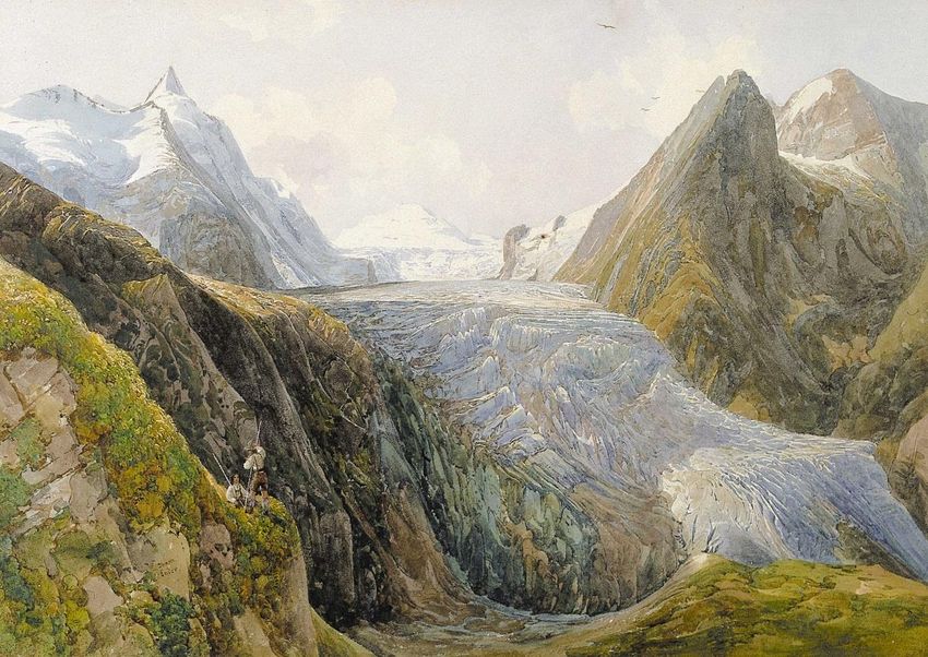
EPJ Web of Conferences 232, 02002 (2020)                                                         https://doi.org/10.1051/epjconf/202023202002
HIAS 2019

                                                                          26
     3.1.3 The Rhone glacier                                                Al (0.72 Myr) was also measured in the samples.
                                                                          Concordant exposure ages for 10Be and 26Al allowed one
     Exposure dating of rock surfaces on Earth by measuring               to make the assumption that the Rhone Glacier removed
     in-situ produced cosmogenic radioisotopes [38, 39] with              several meters of rock during the last Ice Age, leaving the
     Accelerator Mass Spectrometry (AMS) has made it                      sampled bedrock surfaces (Fig. 3) most likely free of
     possible to date glacially polished rock surfaces and glacial        cosmogenic nuclides at the beginning of the Holocene
     moraines. Application of this method allowed one to                  period. Consequently, the measured cosmogenic nuclide
     reconstruct the dynamic history of many glaciers in the              concentration in the sampled material integrates the
     European Alps, and in other glacial regions around the               periods when these rocks were ice-free during the
     world. In particular, if the concentration of two                    Holocene. Since some erosion of the rocks happened also
     radioisotopes with very different half-lives are measured,           during the Holocene, the 10Be exposure ages shown in
     the ratio of these radioisotopes allows one to reconstruct           Fig. 3, decrease toward the lowest, central part of the
     the chronology of glaciers including erosion of the                  glacial trough, where ice velocity was greatest and thus
     underlying bedrock. Such measurements were performed                 erosion rate is expected to be fasted. The longest exposure
     with 14C (t1/2 = 5.7 kyr) and 10Be (1.39 Myr) in quartz              times (4.5 to 5.3 kyr) were found at the left-lateral margin
     grains of recently exposed rock surfaces of the Rhone                zone of the glacier indicating the longest integral time
     Glacier [17], which was one of the dominant glaciers of              when the glacier was smaller than today.
     the European Alps during the Last Ice Age. In addition,

              Figure 3. Sampling location on exposed rocks (darker grey-shaded area) in front of the Rhone Glacier terminus
              (lighter grey-shaded area). Contour lines are labelled in meters a.s.l. The minimum 10Be exposure ages are shown.
              The figure is adopted from the work of Goehring et al. [17].

              Figure 4. Schematic presentation of the time periods where European glaciers were smaller (red) and larger (blue)
              than today. The figure is adapted from the work of Goehring et al. [17]. “Nearby proxy records indicate that at least
              most of the time during which the Rhone glacier was smaller than today was during the early to mid-Holocene” [17].
              In E the hypothetical Holocene advance and retreat scenario of the Rhone Glacier is displayed, indicating the glacier
              was smaller than today during the first part of the Holocene.

                                                                      4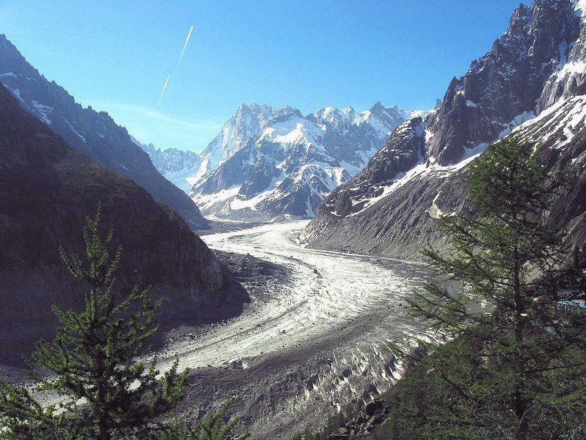
EPJ Web of Conferences 232, 02002 (2020)                                                          https://doi.org/10.1051/epjconf/202023202002
HIAS 2019

     There is also evidence that the ice of the Jostedalsbreen,             3.1.4 The Mer de Glace glacier
     the largest mountain glacier in Norway, is not a left-over
                                                                            A detailed radiocarbon and dendrochronological study was
     from the Last Ice Age, but only formed during the second
                                                                            performed by Le Roy et al. [41] at the Mer de Glace glacier
     half of the Holocene [40]. Although it is unlikely that the
                                                                            in the Mont Blanc massif (Fig. 5A), the largest glacier of
     European Alps were completely ice-free in the early
                                                                            the French Alps. Subfossilized wood exposed at the right
     Holocene, the evidence for generally lower glaciation as
                                                                            lateral moraine near the terminus of the glacier was
     compared to the second half of the Holocene is mounting,
                                                                            investigated (Fig. 5B). It revealed 10 glacial advances
     as indicated from the ice core result from Ortles mentioned
                                                                            during the last ~3000 years. These glacial fluctuations are
     above [36].
                                                                            similar to those observed in the Swiss Alps, although not
                                                                            synchronous in all aspects.

      (A)                                                             (B)

     Figure 5 The lower section of the Mer de Glace glacier in the Mont Blanc mountain range, with the Grandes Jorasse (4208 m a.s.l.) in
     the background (A). The right figure (B) from the work of [41] shows the sampling sites at the right lateral moraine near the glacier
     terminus. Two positions of the terminus in 1995 and 2013, respectively, are marked with black dashed curves. For a detailed description
     of the sampling sites and the material recovered see Ref. [41].

     3.1.5 Timberline
     An important proxy for temperature changes in the Alps
     during the past is the timberline (sometimes also called tree
     line). The timberline is the edge of the habitat at which
     trees can grow (Fig. 6). Since precipitation in the Alps is
     abundant, the movement of the timberline is primarily
     affected by the change in summer temperature during the
     main growing season.
           From studies of subfossil trees preserved at different
     altitudes, periods of higher and lower temperatures,
     respectively, can be reconstructed by 14C measurements
     and dendrochronology. From studies like this (e.g. [12]), it
     has been estimated that the timberline moves                           Figure 6. Typical timberline in an Alpine landscape. The
     approximately 100 m up or down for a summer                            transition from the forested region to grass land can be clearly
     temperature change of ±0.6 oC.                                         seen in this picture, which is reproduced from a free download
                                                                            (https://unsplash.com/s/photos/timberline).

     3.1.6 Temperature change during the Holocene                           Holocene Thermal Maximum (HTM), and continuously
                                                                            decreased in the second half of the Holocene approaching
     In Figure 7, information on glacier and tree-line                      its lowest values during the Little Ice Age (LIA) between
     movements are summarized and converted into                            1300 and 1850 AD. This period also resulted in the largest
     approximate temperature variations during the entire                   glacier advance during the Holocene. The Holocene
     Holocene [22]. Glacial retreats are usually accompanied                temperature trend is also supported by other temperature-
     with higher timberlines indicating higher temperatures.                sensitive proxies, e.g. by the study of chronomids in a
     Overall, the mean temperature went through a maximum                   high-altitude lake (2796 m a.s.l.) in the Austrian Alps [42].
     during the first half of the Holocene, sometimes called the

                                                                       5
EPJ Web of Conferences 232, 02002 (2020) https://doi.org/10.1051/epjconf/202023202002
HIAS 2019
+0.5
∆T (oC) Summer temperature, (May to September)
0
-0.5
-1.0
Iceman
Tree line, higher than today (movement: 100m/0.6oC)
Glacier periods of retreat, Western Alps
Hormes 2001
Joerin 2006
Glacier extent, Eastern Alps
Smaller than today
Advance as in
modern times
BA
Mesolithic Neolithic BA H L RT MA MT
10 9 8 7 6 5 4 3 2 1 BC / AD 1 2
Calibrated date (kiloyears)
Figure 7. Schematic presentation of glacier and tree-line movements in the European Alps during the Holocene [22]. The periods of
smaller glaciers and higher tree lines are indicated with the box symbols. Glacial advances are indicated with filled triangles and curves.
The largest advances took place during the Little Ice Age (~AD 1300 to 1850). The top curve depicts the relative summer temperature
variations deduced mainly from tree-line movements. The mean temperature between AD 1900 and 2000 is used as reference
(ΔT = 0 oC). The red vertical line marks the time where the Iceman Ötzi died [43].
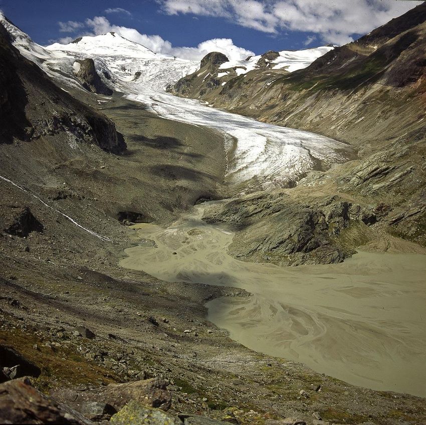
3.2 The New Zealand Southern Alps 3.2.1 The Mueller glacier
Most of the information on Alpine glacier movements The chronology of glacier advances through the past 7000
through the Holocene comes from the Northern years were reconstructed from measurements of
Hemisphere. However, the New Zealand Southern Alps cosmogenic in-situ produced 10Be in moraines of the
allow one to get information on glacier movements in the Mueller glacier, which is located at Mt. Sefton in the Mt.
Southern Hemisphere at comparable latitudes. While Mont Cook mountain range [16]. Figure 8 is reproduced from
Blanc, the highest mountain of the European Alps (4810 m this work and shows the area where the extensive 10Be
a.s.l.) is located at 45.8o N, Aroaki/Mount Cook, the measurements were performed. The deduced exposure
highest mountain of the NZ Southern Alps (3927 m a.s.l.) ages are listed which allow one to draw some conclusions
is located at 43.5o S. Because of the closeness of the Pacific for the glacier advances with respect to the ones in the
Ocean to the East and the Tasman Sea to the West of the European Alps. Interestingly, glacier advances seem not to
NZ Southern Island, the glaciation of the NZ Southern be synchronous between the two hemispheres. Simply
Alps is more intense as compared to the European Alps, speaking, during some time periods glaciers advanced in
even though the latter reach up to considerably higher the Southern Hemisphere (SH) whilst they simultaneously
altitudes. Particularly the western slopes of the NZ retreated in the Northern Hemisphere (NH), and vice
Southern Alps, which are under the influence of the versa.
Tasman Sea and westerlies, are the home of large glaciers As discussed by Schaefer et al. [16], it is possible
(e.g. Fox and Franz Josef glacier), which still reach down that regional effects influenced the pattern of glacier
to about 300 m above sea level. Due to regional cooling, movements in this region. There is, however, some
these two glaciers even advanced during a period of global indication that the oldest ages are found for the most
warming [44]. advanced stages of the glacier. This is more clearly seen in
Here, we describe two rather detailed studies of the chronology of moraines for the Cameron glacier
glacier movements on the eastern side the NZ Southern discussed in the next section (3.2.2).
Alps.
6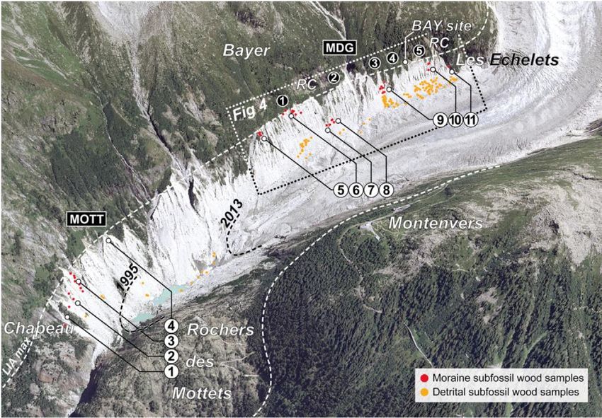
EPJ Web of Conferences 232, 02002 (2020)                                                         https://doi.org/10.1051/epjconf/202023202002
HIAS 2019

                                                            Mt. Sefton
                                                          (3151 m a.s.l.)

       Figure 8. This figure is reproduced from Ref. [16] and shows the results of the 10Be ages (given in years with 2σ uncertainties)
       with the assignment to the Holocene moraines of the Mueller glacier. The ages marked in purple colour are from moraines which
       were deposited during mid- to late-19th century.

                                                                      7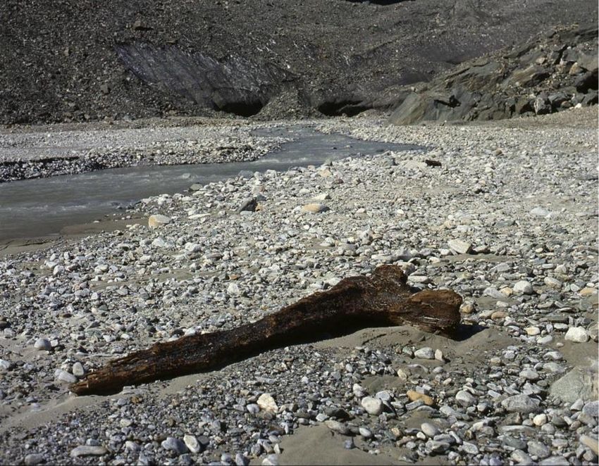
EPJ Web of Conferences 232, 02002 (2020)                                                           https://doi.org/10.1051/epjconf/202023202002
HIAS 2019

     3.2.2 The Cameron glacier                                              interesting conclusion. While in the NH the temperature in
                                                                            the first half of the Holcene is higher than in the second
     Another detailed study of 10Be ages of moraines was                    half, the opposite seems to be the case in the SH. It is
     performed by Putnam et al. [18] at the Cameron glacier in              interesting that this trend is supported by the insolation
     the Arrowsmith Range, which is a smaller mountain range                curves (red curves of panels c and h) calculated from the
     parallel to the Southern Alps about 85 km northeast of                 Milankovic theory of the Earth’s orbital parameter
     Arioka/Mt. Cook. The altitude of the Arrowsmith Range is               variations [45]. Although the insolation changes only by 4
     ~1000 m below the highest ones of the Southern Alps, but               to 6 % over the Holocene, the general temperature trend is
     glaciers are still abundant. Figure 9A show the main results           reproduced. A recent study to take possible effects of
     from the work of Putnam et al. [18], where the moraines                interannual climate variability on the observed glacier
     of the Cameron glacier were dated.                                     fluctuations into account, confirms the robustness of the
           The detailed comparison of temperature proxies of                glacier fluctuations against this short-term climate
     the NH and SH displayed in Fig. 9B [18] leads to an                    fluctuations [46].

      (A)                 Couloir Peak                                      (B)
                          (2624 m a.s.l.)

                                  1930 AD

                                                 520 ± 410
                                  650 ± 30
                            6,890 ± 410       9,200 ± 100

                                               8,100 ± 200

                                                 9,840 ± 470

                                      10,690 ± 410

     Figure 9. In Fig 9A the mean 10Be ages in years (uncertainties 1σ) resulting from the work of Putnam et al. [18] are displayed at the
     Holocene moraines from the Cameron glacier. The oldest age signals the largest glacier advance at the Early Holocene. Fig. 9B shows
     an interesting comparison of various temperatures proxies for the NH (panels a-e) and the SH (panels f-h). For a detailed description of
     Fig. 9B, see Ref. [18].

     4. Conclusions                                                         [18]. The partly asynchronous movements of glaciers in
                                                                            the two hemisphere is probably influenced by regional
     The comparison of glacier movements throughout the                     effects [16].
     Holocene from Alpine mountain ranges in the NH and SH                   This is not surprising considering that the European Alps
     revealed some interesting differences. The opposite                    are largely imbedded into a continental climate, whereas
     temperature development from the Early to the Late                     the NZ Southern Alps are subject to a maritime
     Holocene in the two hemispheres is established by a                    environment.
     number of proxies and supported by the Milankovic theory

                                                                       8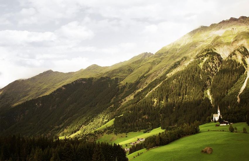
EPJ Web of Conferences 232, 02002 (2020)                                                       https://doi.org/10.1051/epjconf/202023202002
HIAS 2019

           The increasing number of reports about glacier                 to draw more definite conclusions about the influence of
     dynamics in the past from other glaciated regions of the             the sun on the glacier movement during the Holocene.
     Northern and Southern Hemispheres, e.g. from North and                     One thing can be said with some certainty: The
     South America, will help to develop a more concise picture           complex moving patterns of glaciers in both hemispheres
     about climatic variations around the globe during the                of the past have now given way to an accelerated retreat of
     Holocene. Concerning natural causes of the observed                  all glaciers around the globe, most likely due to the
     variations, it is unlikely that they were triggered by               anthropogenic impact on our climate.
     atmospheric CO2 because it was remarkably constant
     throughout the Holocene (Fig. 1 and Ref. [1]). The
     possible influence of solar activity variations has been             Acknowledgement
     discussed [47-49], but since the total solar irradiance
     varies by only ~0.1 % during the Holocene [23], other                We have benefitted from many discussions with
     effects such as volcanic eruptions may have some                     colleagues around the world on the issue of glacier
     influence too. In general, it seems that some amplifying             movements. The wisdom of the late Wally Broecker on
     terrestrial effect are needed to explain the magnitude of the        climate issues is greatly appreciated as an important input
     observed glacier movements. It has to be seen whether the            into the current work.
     recent detailed analysis of solar activity [50] will allow one

     References                                                           [12] K. Nicolussi, M. Kaufmann, G. Patzelt et al.,
                                                                               Holcene tree-line variability in the Kauner Valley,
     [1] The Keeling Curve:                                                    Central       Eastern      Alps,      indicated      by
           https://scripps.ucsd.edu/programs/keelingcurve/                     dendrochronological analysis of living trees and
     [2] S. Arrhenius, On the Influence of Carbonic Acid in                    subfossil logs, Veget. Hist. Archeobot. 14, 221
          the Air upon the Temperature of the Ground, Phil.                    (2005).
          Mag. J. Sci. Ser. 5, 41, 237 (1896).                            [13] U. E. Joerin, T. F. Stocker, and C. Schlüchter,
     [3] P. J. Crutzen and E. F. Stoermer, The Anthropocene,                   Multicentury glacier fluctuations in the Swiss Alps
          The Global Change Newsletters 41, 17 (2000).                         during the Holocene, The Holocene 16, 697 (2006)
     [4] P. J. Crutzen, Geology of mankind, Nature 415, 23                [14] M. Grosjean, P. J. Suter, M. Trachsel et al., Ice-born
          (2002).                                                              prehistoric finds in the Swiss Alps reflect Holocene
     [5] C. N. Waters, J. Zalasiewicz, C. Summerhayes et al.,                  glacier fluctuations, J. Quat. Sci. 22(3), 2003 (2007).
          The       Anthropocene       is    functionally   and           [15] U. E. Joerin, K. Nicolussi, A. Fischer et al., Holocene
          stratigraphically distinct from the Holocene, Science                optimum events inferred from subglacial sediments
          351, 137 (2016).                                                     at Tschierva Glacier, Eastern Alps, Quat. Sci. Rev.
     [6] J. Zalasiewicz, C. N. Waters, P. Wolfe et al., Making                 27(3-4), 337 (2008).
          the case for a formal Anthropocene Epoch: an                    [16] J. M. Schaefer, G. H. Denton, M. Kaplan et al., High-
          analysis of ongoing critiques, Newsletters on                        frequency Holocene glacier fluctuations in New
          Stratigraphy 50(2), 205 (2017).                                      Zealand differ from the northern signature, Science
     [7] F. Höpfel, W. Platzer, and K. Spindler, eds., Der                     324 (5927), 622 (2009).
          Mann im Eis, Band 1. Bericht über das Internationale            [17] B. M. Goehring, J. M. Schaefer, C. Schlüchter et al.,
          Symposium 1992 in Innsbruck, Veröffentlichungen                      The Rhone Glacier was smaller than today for most
          der Universität Innsbruck 187 (1992) pp 464.                         of the Holocene, Geology 39(7), 679 (2011).
     [8] B. Fowler, Iceman – Uncovering the Life and Times                [18] A. E. Putnam, J. M. Schaefer, G. H. Denton et al.,
          of a Prehistoric Man found in an Alpine Glacier,                     Regional climate control of glaciers in New Zealand
          Random House, New York (2000) pp 313.                                and Europe during the pre-industrial Holocene,
     [9] W. Müller, H. Fricke, A. N. Halliday et al., Origin                   Nature Geoscience 5, 628 (2012).
          and migration of the Alpine Iceman, Science 302, 862            [19] I. Schimmelpfenning, J. M. Schaefer, N. Akcar et al.,
          (2003).                                                              Holocene glacier culmination in the Western Alps
     [10] K. Nicolussi, and G. Patzelt., Discovery of Early-                   and their hemispheric relevance, Geology 40, 891
          Holocene wood and peat on the forefield of the                       (2012).
          Pasterze Glacier, Eastern Alps, Austria, The                    [20] I. Schimmelpfenning, J. M. Schaefer, N. Akcar et al.,
          Holocene 10(2), 191 (2000).                                          A chronology of Holocene and Little Ice Age glacier
     [11] A. Hormes, B. U. Müller, and C. Schlüchter, The Alps                 culminations of the Steingletscher, Central Alps,
          with little ice: evidence for eight Holocene phases of               Switzerland, based on high-sensitivity beryllium-10
          reduced glacier extent in the Central Swiss Alps, The                moraine dating, Earth Planet. Sci. Lett. 393, 220
          Holocene 11(3), 255 (2001).                                          (2014).

                                                                      9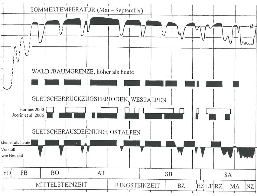
EPJ Web of Conferences 232, 02002 (2020)                                                      https://doi.org/10.1051/epjconf/202023202002
HIAS 2019

     [21] K. Nicolussi and C. Schlüchter, The 8.2 ka event –
          calendar-dated glacier response in the Alps, Geology           [37] T. M. Jenk, S. Szidat, D. Bolius et al., A novel
          40(9), 819 (2014).                                                  Radiocarbon dating technique applied to an ice core
     [22] W. Kutschera, G. Patzelt, P. Steier, and E. M. Wild,                from the Alps indicating late Pleistocene ages, J.
          The Tyrolean Iceman and his glacial environment                     Geophys. Res. 114, D14305 (2009).
          during The Holocene, Radiocarbon 59/2, 395 (2017).             [38] D. Lal, In situ produced cosmogenic isotopes in
     [23] F. Steinhilber, J. Beer, and C. Fröhlich, Total solar               terrestrial rocks, Annu. Rev. Earth Planet. Sci. 16,
          irradiance during the Holocene, Geophys. Res. Lett.                 355 (1988).
          36, L19704 (2009).                                             [39] J. L. Goose, and F. M. Phillips, Terrestrial in situ
     [24] A. Hormes, J. Beer, and C. Schlüchter, A                            cosmogenic nuclides: theory and application, Quat.
          geochronological approach to understand the role of                 Sci. Rev. 20, 1475 (2001).
          solar activity on Holocene glacier length variability          [40] A. Nesje, J. Bakke, S. O. Dahl et al., Norwegian
          in the Swiss Alps, Swiss Alps Geograph. Annals                      mountain glaciers in the past, present and future,
          88A(4), 2281 (2006).                                                Glob. Planet. Change 60, 10 (2008).
     [25] IPCC (Intergovernmental Panel on Climate Change)               [41] M. Le Roy, K. Nicolussi, P. Deline et al., Calendar-
          Special Report on Global Warming of 1.5 oC (2018),                  dated glacier variations in the western European
          https://report.ipcc.ch/sr15/pdf/sr15_spm_final.pdf                  Alps during the Neoglacial: the Mer de Glace record,
     [26] S. E. Koonin, Certainties and uncertainties in our                  Mont Blanc massif, Quat. Sci. Rev. 108, 1 (2015).
          energy and climate future, Schrödinger Lecture,                [42] E. A. Ilyashuk, K. A. Koinig, O. Heiri et al.,
          Austrian Academy of Sciences Vienna (2018),                         Holocene temperature variations at a high-altitude
          unpublished.                                                        site in the Eastern Alps: A chironomid record from
     [27] P. J. Crutzen, Albedo enhancement by stratospheric                  Schwarzsee ob Sölden, Austria, Quat. Sci. Rev. 30,
          sulfur injections: a contribution to resolve a policy               176 (2011).
          dilemma? Climate Change 77, 211 (2006).                        [43] W. Kutschera, G. Patzelt, E. M. Wild et al., Evidence
     [28] P. Ramond, Murray Gell-Man (1929-2019), Science                     for early human presence at high altitudes in the
          364, 1236 (2019).                                                   Ötztal Alps (Austria/Italy), Radiocarbon 56/3, 923
     [29] L. Augustin, C. Barbante, P. R. F. Barnes et al., Eight             (2017).
          glacial cycles from an Antarctic ice core, Nature 429,         [44] A. N. Mackintosh, B. M. Anderson, A. M. Lorrey et
          623 (2004).                                                         al. Regional cooling caused recent New Zealand
     [30] J. Jouzel, V. Masson-Delmotte, O. Cattani et al.,                   glacier advances in a period of global warming,
          Orbital and millennial Antarctic climate variability                Nature Comms. 8, 14202 (2017).
          over the past 800,000 years, Science 317, 793 (2007).          [45] M. Milankovic, Kanon der Erdbestrahlung und seine
     [31] J. D. Hays, J. Imbrie, and N. J. Shackleton,                        Anwendung auf das Eiszeitenproblem, Königliche
          Variations in the Earth's Orbit: Pacemaker of the Ice               Serbische Akademie, Belgrad (1941), English
          Ages, Science 194, 1121 (1976).                                     translation, Canon of Insolation and the Ice-Age
     [32] O. Passalacqua, M. Cavitte, O. Gagliardini et al.,                  Problem, Belgrade (1998) pp 634.
          Brief communication: Candidate sites of 1.5 Myr old            [46] A. M. Doughty, A. N. Mackintosh, B. M. Anderson
          ice 37 km southwest of the Dome C summit, East                      et al., An exercise in glacier length modeling:
          Antarctica, The Cryosphere 12, 2167 (2018).                         Interannual climatic variability alone cannot explain
     [33] N. B. Karlsson, T. Binder, G. Eagles et al.,                        Holocene glacier fluctuations in New Zealand, Earth
          Glaciological characteristics in the Dome Fuji                      Planet. Sci. Lett. 470, 48 (2017).
          region and new assessment for “Oldest Ice”, The                [47] F. Steinhilber, J. A. Abreu, J. Beer et al., 9,400 years
          Cryosphere 12, 2413 (2018).                                         of cosmic radiation and solar activity from ice cores
     [34] Temperature            of        Planet         Earth,              and tree rings, PNAS 109/16, 5967 (2012).
          https://en.wikipedia.org/wiki/File:All_palaeotemps.            [48] J. A. Abreu, J. Beer, F. Steinhilber et al., 10Be in ice
          png                                                                 cores and 14C in tree rings: separation of production
     [35] G. L. Foster, D. L. Royer, and D. J. Lunt, Future                   and climate effects, Space Sci. Rev. 176(1), 343
          climate forcing potentially without precedent in the                (2013).
          last 420 million years, Nature Comm. 8:14845                   [49] A. P. Schurer, S. F. B. Tett, and G. C. Hegerl, Small
          (2017).                                                             influence of solar variability on climate over the past
     [36] P. Gabrielli, C. Barbante, G. Bertagna et al., Age of               millennium, Nature Geoscience 7, 104 (2014).
          the Mt. Ortles ice cores, the Tyrolean Iceman and              [50] C. J. Wu, I. G. Usokin, N. Krivova et al., Solar
          glaciation of the highest summit of South Tyrol                     activity over nine millennia: A consistent multi-proxy
          since the Northern Hemisphere Climatic Optimum,                     reconstruction, Astron. & Astrophys. 615, A93
          The Cryosphere 10, 2779 (2016).                                     (2018).

                                                                    10
You can also read