The Unreasonable Effectiveness of the Final Batch Normalization Layer
←
→
Page content transcription
If your browser does not render page correctly, please read the page content below
The Unreasonable Effectiveness of the
                                                                        Final Batch Normalization Layer

                                                      Veysel Kocaman1                             Ofer M. Shir2                     Thomas Bäck1

                                                                         1 LIACS,
                                                                                Leiden University, Leiden, The Netherlands
                                                    2 Computer   Science Department, Tel-Hai College and Migal Institute, Upper Galilee, Israel
arXiv:2109.09016v1 [cs.CV] 18 Sep 2021

                                                             Abstract                                    1   INTRODUCTION

                                                                                                         Detecting anomalies that are hardly distinguishable from
                                         Early-stage disease indications are rarely recorded             the majority of observations is a challenging task that of-
                                         in real-world domains, such as Agriculture and                  ten requires strong learning capabilities since anomalies
                                         Healthcare, and yet, their accurate identification is           appear scarcely, and in instances of diverse nature, a labeled
                                         critical in that point of time. In this type of highly          dataset representative of all forms is typically unattainable.
                                         imbalanced classification problems, which encom-                Despite tremendous advances in computer vision and object
                                         pass complex features, deep learning (DL) is much               recognition algorithms in the past few years, their effec-
                                         needed because of its strong detection capabili-                tiveness remains strongly dependent upon the datasets’ size
                                         ties. At the same time, DL is observed in practice              and distribution, which are usually limited under real-world
                                         to favor majority over minority classes and con-                settings. This work is mostly concerned with hard classifi-
                                         sequently suffer from inaccurate detection of the               cation problems at early-stages of abnormalities in certain
                                         targeted early-stage indications. In this work, we              domains (i.e. crop, human diseases, chip manufacturing),
                                         extend the study done by [Kocaman et al., 2020],                which suffer from lack of data instances, and whose effective
                                         showing that the final BN layer, when placed be-                treatment would make a dramatic impact in these domains.
                                         fore the softmax output layer, has a considerable               For instance, fungus’s visual cues on crops in agriculture
                                         impact in highly imbalanced image classification                or early-stage malignant tumors in the medical domain are
                                         problems as well as undermines the role of the soft-            hardly detectable in the relevant time-window, while the
                                         max outputs as an uncertainty measure. This cur-                highly infectious nature leads rapidly to devastation in a
                                         rent study addresses additional hypotheses and re-              large scale. Other examples include detecting the faults in
                                         ports on the following findings: (i) the performance            chip manufacturing industry, automated insulation defect
                                         gain after adding the final BN layer in highly im-              detection with thermography data, assessments of installed
                                         balanced settings could still be achieved after re-             solar capacity based on earth observation data, and nature
                                         moving this additional BN layer in inference; (ii)              reserve monitoring with remote sensing and deep learning.
                                         there is a certain threshold for the imbalance ra-              However, class imbalance poses an obstacle when address-
                                         tio upon which the progress gained by the final                 ing each of these applications.
                                         BN layer reaches its peak; (iii) the batch size also
                                         plays a role and affects the outcome of the final               In recent years, reliable models capable of learning from
                                         BN application; (iv) the impact of the BN appli-                small samples have been obtained through various ap-
                                         cation is also reproducible on other datasets and               proaches, such as autoencoders [Beggel et al., 2019], class-
                                         when utilizing much simpler neural architectures;               balanced loss (CBL) to find the effective number of samples
                                         (v) the reported BN effect occurs only per a single             required [Cui et al., 2019], fine tuning with transfer learn-
                                         majority class and multiple minority classes – i.e.,            ing [Hussain et al., 2018], data augmentation [Shorten and
                                         no improvements are evident when there are two                  Khoshgoftaar, 2019], cosine loss utilizing (replacing cate-
                                         majority classes; and finally, (vi) utilizing this BN           gorical cross entropy) [Barz and Denzler, 2020], or prior
                                         layer with sigmoid activation has almost no impact              knowledge [Lake et al., 2015].
                                         when dealing with a strongly imbalanced image                    [Kocaman et al., 2020] presented an effective modifica-
                                         classification tasks.                                           tion in the neural network architecture, with a surprising
                                                                                                         simplicity and without a computational overhead, which en-

                                                             Accepted for the 16th International Symposium on Visual Computing (ISVC 2021).
ables a substantial improvement using a smaller number of               MNIST dataset, reproduced the same BN impact, and
anomaly samples in the training set. The authors empirically            furthermore demonstrated that the final BN layer has a
showed that the final BN layer before the softmax output                considerable impact not just in modern CNN architec-
layer has a considerable impact in highly imbalanced image              tures but also in simple CNNs and even in one-layered
classification problems. They reported that under artificially-         feed-forward fully connected (FC) networks.
generated skewness of 99% vs. 1% in the PlantVillage (PV)
                                                                      • We illustrate that the performance gain occurs only
image dataset [Mohanty et al., 2016], the initial F1 test score
                                                                        when there is a single majority class and multiple mi-
increased from the 0.29-0.56 range to the 0.95-0.98 range
                                                                        nority classes; and no improvement observed regard-
(almost triple) for the minority class when BN modifica-
                                                                        less of the final BN layer when there are two majority
tion applied. They also argued that, a model might perform
                                                                        classes.
better even if it is not confident enough while making a pre-
diction, hence the softmax output may not serve as a good             • We argue that using the final BN layer with sigmoid
uncertainty measure for DNNs (see Figure 1).                            activation has almost no impact when dealing with a
                                                                        strongly imbalanced image classification tasks.
This shows that DNNs have the tendency of becoming ‘over-
confident’ in their predictions during training, and this can
                                                                  The remainder of the paper is organized as follows: Sec-
reduce their ability to generalize and thus perform as well
                                                                  tion 2 gives some background concerning the role of the BN
on unseen data. In addition, large datasets can often com-
                                                                  layer in neural networks. Section 3 summarizes the previous
prise incorrectly labeled data, meaning inherently the DNN
                                                                  findings and existing hypotheses in the previous work done
should be a bit skeptical of the ‘correct answer’ to avoid
                                                                  by [Kocaman et al., 2020] and then lists the derived hypothe-
being overconfident on bad answers. This was the main mo-
                                                                  ses that will be addressed throughout this study. Section 4
tivation of Müller et al. [Müller et al., 2019] for proposing
                                                                  elaborates the implementation details and settings for our
the label smoothing, a loss function modification that has
                                                                  new experiments and presents results. Section 5 discusses
been shown to be effective for training DNNs. Label smooth-
                                                                  the findings and proposes possible mechanistic explanations.
ing encourages the activations of the penultimate layer to
                                                                  Section 6 concludes this paper by pointing out key points
be close to the template of the correct class and equally dis-
                                                                  and future directions.
tant to the templates of the incorrect classes [Müller et al.,
2019]. Despite its relevancy, [Kocaman et al., 2020] also
reports that label smoothing did not do well in their study as    2    BACKGROUND
previously mentioned by Kornblith et al. [Chelombiev et al.,
2019] who demonstrated that label smoothing impairs the           In order to better understand the novel contributions of this
accuracy of transfer learning, which similarly depends on         study, in this section, we give some background information
the presence of non-class-relevant information in the final       about the Batch Normalization (BN) [Ioffe and Szegedy,
layers of the network.                                            2015] concept. Since the various applications of BN in sim-
In this study, we extend previous efforts done by [Koca-          ilar studies and related work have already been investigated
man et al., 2020] to devise an effective approach to enable       thoroughly in our previous work [Kocaman et al., 2020], we
learning of minority classes, given the surprising evidence       will only focus on the fundamentals of BN in this chapter.
of applying the final Batch Normalization (BN) layer.             Training deep neural networks with dozens of layers is chal-
Given these recent findings, we formulate and test additional     lenging as the networks can be sensitive to the initial random
hypotheses and report our observations in what follows. The       weights and configuration of the learning algorithm. One
concrete contributions of this paper are the following:           possible reason for this difficulty is that the distribution
                                                                  of the inputs to layers deep in the network may change
   • The performance gain after adding the final BN layer in      after each mini-batch when the weights are updated. This
     highly imbalanced settings could still be achieved after     slows down the training by requiring lower learning rates
     removing this additional BN layer during inference; in       and careful parameter initialization, makes it notoriously
     turn enabling us to get a performance boost with no          hard to train models with saturating nonlinearities [Ioffe and
     additional cost in production.                               Szegedy, 2015], and can cause the learning algorithm to
                                                                  forever chase a moving target. This change in the distribu-
   • There is a certain threshold for the ratio of the im-        tion of inputs to layers in the network is referred to by the
     balance for this specific PV dataset, upon which the         technical name “internal covariate shift” (ICS).
     progress is the most obvious after adding the final BN
     layer.                                                       BN is a widely adopted technique that is designed to combat
                                                                  ICS and to enable faster and more stable training of deep
   • The batch size also plays a role and significantly affects
                                                                  neural networks (DNNs). It is an operation added to the
     the outcome.
                                                                  model before activation which normalizes the inputs and
   • We replicated the similar imbalanced scenarios in            then applies learnable scale (γ) and shift (β ) parameters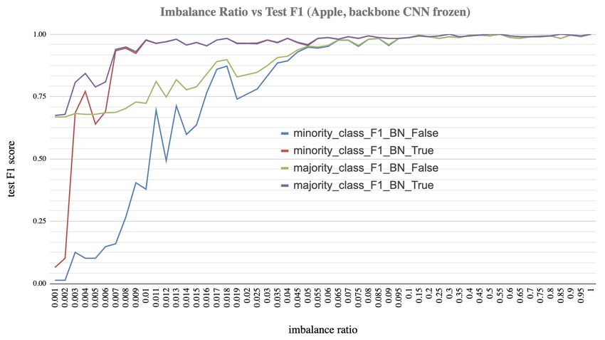
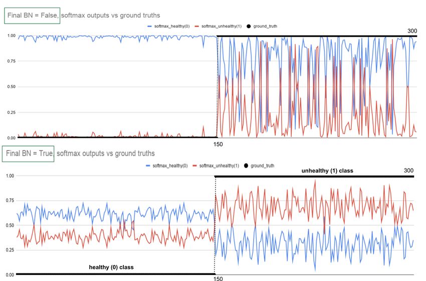
Figure 1: The x-axis represents the ground truth for all 150 healthy (0) and 150 unhealthy (1) images in the test set while red
and blue lines represent final softmax output values between 0 and 1 for each image. Top chart (without final BN): When
ground truth (black) is class = 0 (healthy), the softmax output for class = 0 is around 1.0 (blue, predicting correctly). But
when ground truth (black) is class = 1 (unhealthy), the softmax output for class = 1 (red points) changes between 0.0 and
1.0 (mostly below 0.5, NOT predicting correctly). Bottom chart (with final BN): When ground truth (black) is class = 0
(healthy), the softmax output is between 0.5 and 0.75 (blue, predicting correctly). When ground truth (black) is class = 1
(unhealthy), the softmax output (red points) changes between 0.5 and 1.0 (mostly above 0.5, predicting correctly).

to preserve model performance. Given m activation values           distributional stability of layer inputs has little to do with
x1 . . . , xm from a mini-batch B for any particular layer input   the success of BN and the relationship between ICS and
x( j) and any dimension j ∈ {1, . . . , d}, the transformation     BN is tenuous. Instead, they uncovered a more fundamental
uses the mini-batch mean µB = 1/m ∑m        i=1 xi and variance    impact of BN on the training process: it makes the opti-
  2 = 1/m m (x − µ )2 for normalizing the x according              mization landscape significantly smoother. This smoothness
σB              ∑i=1 iq B                            i

to x̂i = (xi − µB )/ σB  2 + ε and then applies the scale and      induces a more predictive and stable behavior of the gradi-
                                                                   ents, allowing for faster training. Bjorck et al. [Bjorck et al.,
shift to obtain the transformed values yi = γ x̂i + β . The con-
                                                                   2018] also makes similar statements that the success of BN
stant ε > 0 assures numerical stability of the transformation.
                                                                   can be explained without ICS. They argue that being able to
BN has the effect of stabilizing the learning process and dra-     use larger learning rate increases the implicit regularization
matically reducing the number of training epochs required          of the gradient, which improves generalization.
to train deep networks; and using BN makes the network
                                                                   Even though BN adds an overhead to each iteration (esti-
more stable during training. This may require the use of
                                                                   mated as additional 30% computation [Mishkin and Matas,
much larger learning rates, which in turn may further speed
                                                                   2015]), the following advantages of BN outweigh the over-
up the learning process.
                                                                   head shortcoming:
Though BN has been around for a few years and has become
common in deep architectures, it remains one of the DL                • It improves gradient flow and allows training deeper
concepts that is not fully understood, having many studies              models (e.g., ResNet).
discussing why and how it works. Most notably, Santurkar et
al. [Santurkar et al., 2018] recently demonstrated that such          • It enables using higher learning rates because it elim-
                                                                        inates outliers’ activation, hence the learning process
may be accelerated using those high rates. predicted probabilities. In their implementation, they added
• It reduces the dependency on initialization and then re- another 2-input BN layer after the last dense layer (before
duces overfitting due to its minor regularization effect. softmax output) in addition to existing BN layers in the tail
Similarly to dropout, it adds some noise to each hidden and 4 BN layers in the head of the DL architecture (e.g.,
layer’s activation. ResNet34 possesses a BN layer after each convolutional
layer, having altogether 38 BN layers given the additional 4
• Since the scale of input features would not differ sig- in the head).
nificantly, the gradient descent may reduce the oscil-
lations when approaching the optimum and thus con- At first they run experiments with VGG19 architectures for
verge faster. selected plant types by adding the final BN layer. When they
train this model for 10 epochs and repeat this for 10 times,
• BN reduces the impacts of earlier layers on the follow-
they observed that the F1 test score is increased from 0.2942
ing layers in DNNs. Therefore, it takes more time to
to 0.9562 for unhealthy Apple, from 0.7237 to 0.9575 for
train the model to converge. However, the use of BN
unhealthy Pepper and from 0.5688 to 0.9786 for unhealthy
can reduce the impact of earlier layers by keeping the
Tomato leaves. They also achieved significant improvements
mean and variance fixed, which in some way makes
in healthy samples (being the majority in the training set).
the layers independent from each other. Consequently,
See Table 1 for details.
the convergence becomes faster.
3 PREVIOUS FINDINGS AND EXISTING 3.2 EXPERIMENTATION ON PLANTVILLAGE
HYPOTHESES DATASET SUBJECT TO DIFFERENT
CONFIGURATIONS
In the work done by [Kocaman et al., 2020], the authors fo-
cused their efforts on the role of BN layer in DNNs, where Using the following six configuration variations with two
in the first part of the experiments ResNet34 [Simonyan options each, the authors created 64 different configurations
and Zisserman, 2014] and VGG19 CNN architectures [He which they tested with ResNet34 (training for 10 epochs
et al., 2016] are utilized. They first addressed the complete only): Adding (X) a final BN layer just before the output
PV original dataset and trained a ResNet34 model for 38 layer (BN), using (X) weighted cross-entropy loss [Goodfel-
classes. Using scheduled learning rates [Smith, 2017], they low et al., 2016] according to class imbalance (WL), using
obtained 99.782% accuracy after 10 epochs – slightly im- (X) data augmentation (DA), using (X) mixup (MX) [Zhang
proving the PV project’s record of 99.34% when employing et al., 2017], unfreezing (X) or freezing (learnable vs pre-
GoogleNet [Mohanty et al., 2016]. In what follows, we sum- trained weights) the previous BN layers in ResNet34 (UF),
marize the previous observations borrowed from [Kocaman and using (X) weight decay (WD) [Krogh and Hertz, 1992].
et al., 2020] and then formulate the derived hypotheses that Checkmarks (X) and two-letter abbreviations are used in
became the core of the current study. Table 2 to denote configurations. When an option is disabled
across all configurations, its associated column is dropped.
3.1 ADDING A FINAL BATCH NORM LAYER As shown in Table 2, just adding the final BN layer was
BEFORE THE OUTPUT LAYER enough to get the highest F1 test score in both classes. Sur-
prisingly, although there is already a BN layer after each con-
By using the imbalanced datasets for certain plant types volutional layer in the backbone CNN architecture, adding
(1,000/10 in the training set, 150/7 in the validation set and one more BN layer just before the output layer boosts the
150/150 in the test set), [Kocaman et al., 2020] performed test scores. Notably, the 3rd best score (average score for
several experiments with the VGG19 and ResNet34 archi- configuration 31 in Table 2) is achieved just by adding a
tectures. The selected plant types were Apple, Pepper and single BN layer before the output layer, even without un-
Tomato - being the only datasets of sufficient size to enable freezing the previous BN layers.
the 99%-1% skewness generation. All the tests are run with
One of the important observations is that the model with-
batch size 64.
out the final BN layer is pretty confident even if it predicts
In order to fine-tune the network for the PV dataset, the falsely. But the proposed model with the final BN layer
final classification layer of CNN architectures is replaced predicts correctly even though it is less confident. They
by Adaptive Average Pooling (AAP), BN, Dropout, Dense, basically ended up with less confident but more accurate
ReLU, BN and Dropout followed by the Dense and BN models in less than 10 epochs. The classification proba-
layer again. The last layer of an image classification net- bilities for five sample images from the unhealthy class
work is often a FC layer with a hidden size being equal (class = 1) with final BN layer (right column) and without
to the number of labels to output the predicted confidence final BN layer (left column) are shown in Table 3. As ex-
scores that are normalized by the softmax operator to obtain plained above, without the final BN layer, these anomaliesTable 1: Averaged F1 test set performance values over 10 runs, alongside BN’s total improvement, using 10 epochs with
VGG19, with/without BN and with Weighted Loss (WL) without BN.
without final with WL with final BN BN total
plant class
BN (no BN) (no WL) improvement
Apple Unhealthy 0.2942 0.7947 0.9562 0.1615
Healthy 0.7075 0.8596 0.9577 0.0981
Pepper Unhealthy 0.7237 0.8939 0.9575 0.0636
Healthy 0.8229 0.9121 0.9558 0.0437
Tomato Unhealthy 0.5688 0.8671 0.9786 0.1115
Healthy 0.7708 0.9121 0.9780 0.0659
Table 2: Best performance metrics over the Apple dataset under various configurations using ResNet34.
Config Test set Test set Test set
Class Epoch BN DA UF WD
Id precision recall F1-score
Unhealthy 31 0.9856 0.9133 0.9481 6 X
(class = 1) 23 0.9718 0.9200 0.9452 6 X X
20 0.9926 0.8933 0.9404 7 X X X X
are all falsely classified (recall that Psoftmax (class = 0) = iteration (mini-batch), its sizing could also play a role
1 − Psoftmax (class = 1)). on the level of progress with the final BN layer.
• The observations and performance gain with respect
Table 3: Softmax output values (representing class proba- to the PV dataset, upon utilizing ResNet and VGG
bilities) for five sample images of unhealthy plants. Left architectures, may not be reproduced with any other
column: Without final BN layer, softmax output values for dataset or with much simpler neural architectures.
unhealthy, resulting in a wrong classification in each case.
Right column: With final BN layer, softmax output value • Since the number of units in the output layer depends
for unhealthy, resulting in correct but less "confident" clas- on the number of classes in the dataset, the perfor-
sifications. mance gain may not be achieved in multi-classification
settings and the number of majority and minority
classes can affect the role of the final BN layer.
Without final BN layer With final BN layer
• Since sigmoid activation is also one of the most widely
0.1082 0.5108 used activation functions in the output layer for the
0.1464 0.6369 binary classification problems, the performance gain
0.1999 0.6082 could be achieved with sigmoid outputs as well.
0.2725 0.6866
0.3338 0.7032 Next, we report on addressing these hypotheses, one by one,
and describe our empirical findings in detail.
3.3 DERIVED HYPOTHESES
4 IMPLEMENTATION DETAILS AND
Under all these observations and findings mentioned above,
EXPERIMENTAL RESULTS
we derived the following hypotheses for our new study:
4.1 REMOVING THE ADDITIONAL BN LAYER
• The added complexity to the network by adding the DURING INFERENCE (H-1)
final BN layer could be eliminated by removing the
final BN layer in inference without compromising the Since adding the final BN layer adds a small overhead (four
performance gain achieved. new parameters) to the network at each iteration, we exper-
imented if the final BN layer could be dropped once the
• There might be a certain level of skewness upon which training is finished so that we can avoid the cost. Dropping
the progress reaches its peak without further sizing the this final BN layer means that training the network from end
minority class. to end, and then chopping off the final BN layer from the
• Since the trainable parameters in a BN layer also de- network before saving the weights. We tested this hypothe-
pend on the batch size (i.e., number of samples) in each sis for Apple, Pepper and Tomato images from PV datasetunder three conditions with 1% imbalance ratio: Without fi- score is gained when the batch size is around 64, whereas the
nal BN, with final BN and then removing the final BN during accuracy drops afterwards with larger batches. The results
testing. We observed that removing the final BN layer in in- are exhibited in Figure 2b. Consequently, given the reported
ference would still give us a considerable boost on minority observations, we confirm hypotheses (H-2) and (H-3).
class without losing any performance gain on the majority
class. The results in Table 4 show that the performance gain
is very close to the configuration in which we used the final 4.3 EXPERIMENTATION ON THE MNIST
BN layer both in training and inference time. As a conse- DATASET: THE IMPACT OF FINAL BN
quence, we confirm hypothesis (H-1) by showing that the LAYER IN BASIC CNNS AND FC NETWORKS
final BN layer can indeed be removed in inference without [(H-4),(H-5),(H-6)]
compromising the performance gain.
In order to reproduce equivalent results on a well known
benchmark dataset when utilizing different DL architectures,
4.2 IMPACT LEVEL REGARDING THE we set up two simple DL architectures: a CNN network with
IMBALANCE RATIO (H-2) AND THE BATCH five Conv2D layers and a one-layer (128-node) FC feed for-
SIZE (H-3) ward NN. Then we sampled several pairs of digits (2 vs 8, 3
vs 8, 3 vs 5 and 5 vs 8) from MNIST dataset that are mostly
confused in a digit recognition task due to similar patterns
[Kocaman et al., 2020] empirically shows that the final BN
in the pixels. During the experiments, the ratio of minority
layer, when placed be-fore the softmax output layer, has a
class to majority is kept as 0.1 and experiments with the
considerable impact in highly imbalanced image classifica-
simple CNN architecture indicates that, after adding the
tion problems but they fail to explain the impact of using
final BN layer, we gain ∼ 20% boost in minority class and
the final BN layer as a function of level of imbalance in
∼ 10% in majority class (see Table 5). Lower standard devi-
the training set. In order to find if there is a certain ratio in
ations across the runs with final BN layer also indicates the
which the impact is maximized, we tested this hypothesis
regularization effect of using the final BN layer. As a result,
(H-1) over various levels of imbalance ratios and condi-
we rejected the fourth hypothesis (H-4) that we derived in
tions explained below. In sum, we ended up with 430 model
section 3.3 by showing that the performance gain through
runs, each with 10 epochs (basically tested with 5, 10, 15, ..
the final BN layer can be reproduced with another dataset or
100 unhealthy vs 1000 healthy samples). During the experi-
with much simpler neural architectures. Another important
ments, we observed that the impact of final BN on highly
finding is that the final BN layer boosts the minority class’
imbalanced settings is the most obvious when the ratio of
F1 scores only when there is a single majority class. When
minority class to the majority is less than 10%; above that
two majority classes are set, no improvements are evident
almost no impact. As expected, the impact of the final BN
regardless of the usage of the final BN layer (see 4th and 5th
layer is more obvious on minority class than it is on majority
settings in Table 6). Therefore, we partially confirm hypoth-
class, albeit the level of impact with respect to the imbal-
esis (H-5) by showing that the performance gain through the
ance ratio is almost same, and levels off around 10%. It is
final BN layer can also be achieved in multi-classification
mainly because of the fact that the backbone architecture
settings but the number of majority and minority classes
(ResNet34) is already good enough to converge faster on
may affect the role of the final BN layer. In the experiments
such data set (Plant Village) and the model does well on
with a one-layer FC network, we enriched the scope and
both classes after 10% imbalance (having more than 100
also tested whether using different loss functions and out-
unhealthy with respect to 1000 healthy samples can already
put activation functions would have an impact on model
be handled regardless of final BN trick). During these ex-
performance using final BN layer with or without another
periments, we also tested if unfreezing the previous layers
BN layer after the hidden layer. We observed that adding
in the backbone CNN architecture (ResNet34) would also
the final BN layer, softmax output layer and categorical
matter. We observed that unfreezing the pretrained layers
crossentropy (CCE) as a loss function have the highest test
helps without even final BN layer, but unfreezing adds more
F1 scores for both classes. It is also important to note that
computation as the gradient loss will be calculated for each
we observe no improvement even after adding the final BN
one of them. After adding the final BN layer and freezing
layer when we use sigmoid activation in the output layer
the previous pretrained layers, we observed similar metrics
(Table 6). Accordingly, we reject hypothesis (H-6).
and learning pattern as we did with unfreezing but not with
final BN layer. This is another advantage of using the final
BN that allow us to freeze the previous pretrained layers.
5 DISCUSSION
The results are displayed as charts in Figure 2a.
We also experimented if the batch size would also be an In a previous work done in [Kocaman et al., 2020], the
important parameter for the minority class test accuracy authors suggested that by applying BN to dense layers, the
when the final BN is added and found out that the highest gap between activations is reduced (normalized) and thenTable 4: Training with the final BN layer, and then dropping this layer while evaluating on the test set proved to be still
useful in terms of improving the classification score on minority classes, albeit not as much as with the final BN layer kept
(imbalance ratio 0.01, epoch 10, batch size 64).
Apple Pepper Tomoto
healthy unhealthy healthy unhealthy healthy unhealthy
with no final BN 0.71 0.22 0.74 0.45 0.74 0.46
with final BN 0.92 0.91 0.94 0.94 0.98 0.98
train with final BN 0.74 0.83 0.75 0.82 0.78 0.85
remove while testing
(a) The impact of final BN layer on the F1 test score of each class (b) The impact of batch size on the F1 test score when the final
for Apple plant. The impact is the most obvious when the ratio of BN layer added. The highest score is gained when the batch size
minority class to the majority is less than 0.1. is 64 and then the accuracy starts declining.
Figure 2: Imbalance ratio and batch size analysis with respect to the final BN layer added
Table 5: Average test metrics with a simple CNN network In this study, we empirically demonstrated that the final BN
(5xConv2D) to classify 3 (minority) and 8 (majority) images layer could still be eliminated in inference without compro-
from MNIST dataset with 0.01 imbalance ratio, 10 runs, and mising the attained performance gain. This finding supports
20 epoch per run. the assertion that adding the BN layer makes the optimiza-
tion landscape significantly smoother, which in turn renders
with BN without BN with BN without BN the gradients’ behavior more predictive and stable – as sug-
minority minority majority majority
gested by [Santurkar et al., 2018]. We argue that the learned
Test F1 0.9299 0.7378 0.9447 0.8354 parameters, which were affected by the addition of the final
Std. Dev. 0.0791 0.1126 0.0487 0.0506 BN layer under imbalanced settings, are likely sufficiently
robust to further generalization on the unseen samples, even
without normalization prior to the softmax layer.
softmax is applied on normalized outputs, which are cen- The observation of locating a sweet spot (10%) for the
tered around the mean. Therefore, ending up with centered imbalance ratio, at which we can utilize the final BN layer,
probabilities (around 0.5), but favoring the minority class might be explained by the fact that the backbone ResNet
by a small margin. They also argued that DNNs have the architecture is already strong enough to easily generalize
tendency of becoming ‘over-confident’ in their predictions on the PV dataset and the model does not need any other
during training, and this can reduce their ability to general- regularization once the number of samples from the minority
ize further and thus perform as well on unseen data. Then class exceeds a certain threshold. As the threshold found in
they also concluded that a DNN with the final BN layer is our experiments is highly related to the DL architecture and
more calibrated [Guo et al., 2017]. We assert that ’being the utilized dataset, it is clear that it may not apply to other
less confident’ in terms of softmax outputs might be fun- datasets, but can be found in a similar way.
damentally wrong and a network shouldn’t be discarded or As discussed before, the BN layer calculates mean and vari-
embraced due to its capacity of producing confident or less ance to normalize the previous outputs across the batch,
confident results in the softmax layer as it may not even be whereas the accuracy of this statistical estimation increases
interpreted as a ’confidence’.Table 6: Using the same ResNet-34 architecture and skewness (1% vs 99%) and setting up five different configurations
across various confusing classes from MNIST dataset, it is clear that adding the final BN layer boosts the minority class
F1 scores by 10% to 30% only when there is a single majority class. When we have two majority classes, there is no
improvement observed regardless of the final BN layer is used or not. (X) indicates minority classes.
Setting-1 Setting-2 Setting-3 Setting-4 Setting-5
3 (X) 8 2 (X) 8 3 (X) 5 3 (X) 5 8 3 (X) 5 (X) 8
without final BN 0.19 0.69 0.25 0.70 0.24 0.70 0.06 0.77 0.78 0.28 0.32 0.56
with final BN 0.55 0.76 0.50 0.74 0.54 0.76 0.00 0.77 0.78 0.58 0.59 0.69
Table 7: Using one-layer (128 node) NN and the 0.01 skew- We at first noticed that the performance gain after adding
ness ratio, with nine different settings for 3 (minority) and 8 the final BN layer in highly imbalanced settings could still
(majority) classes from MNIST dataset (100-epoch). Adding be achieved after removing this additional BN layer during
the final BN layer, softmax output layer and CCE as a loss inference; in turn enabling us to get a performance boost
function has the highest test F1 scores for both classes. (CCE with no additional cost in production. Then we explored
- categorical cross entropy, BCE - binary cross entropy, first the dynamics of using the final BN layer as a function of
BN - a BN layer after the hidden layer). the imbalance ratio within the training set, and found out
that the impact of final BN on highly imbalanced settings
output loss first final class-3 class-8 is the most apparent when the ratio of minority class to the
activation function BN layer BN layer (minority) (majority)
majority is less than 10%; there is hardly any impact above
sigmoid BCE 0.17 0.67
softmax BCE 0.00 0.67
that threshold.
softmax BCE X 0.60 0.78 We also ran similar experiments with simpler architectures,
softmax CCE 0.67 0.80
sigmoid BCE X 0.05 0.67 namely a basic CNN and a single-layered FC network, when
softmax BCE X 0.85 0.88 applied to the MNIST dataset under various imbalance set-
softmax BCE X X 0.83 0.87 tings. The simple CNN experiments exhibited a gain of ∼
softmax CCE X 0.88 0.90 20% boost per the minority class and ∼ 10% per the major-
softmax CCE X X 0.78 0.85
ity class after adding the final BN layer. In the FC network
experiments, we observed improvements by 10% to 30%
only when a single majority class was defined; no improve-
as the batch size grows. However, its role seems to change ments were evident for two majority classes, regardless of
under the imbalanced settings – we found out that a batch the usage of the final BN layer. While experimenting with
size of 64 reaches the highest score, whereas by utilizing different activation and cost functions, we found out that
larger batches the score consistently drops. As a possible using the final BN layer with sigmoid activation had almost
explanation for this observation, we think that the larger no impact on the task at hand.
the batches, the higher the number of majority samples in a
batch and the lesser the chances that the minority samples We found the impact of final BN layer in simpler neural
are fairly represented, resulting in a deteriorated perfor- networks quite surprising. It is an important finding, which
mance. we plan to further investigate in the future, as it requires
thorough analysis. We also plan to formulate our findings
During our experiments, we expected to see similar behav- in a generalized way for any neural model, preferably with
ior with sigmoid activation replacing softmax in the output a combination of softmax activation or a proper loss func-
layer, but, evidently, the final BN layer works best with soft- tion that could be used in imbalanced image classification
max activations. Although softmax output may not serve as problems.
a good uncertainty measure for DNNs compared to sigmoid
layer, it can still do well on detecting the under-represented
samples when used with the final BN layer. REFERENCES
Bjorn Barz and Joachim Denzler. Deep learning on small
6 CONCLUSIONS datasets without pre-training using cosine loss. In The
IEEE Winter Conference on Applications of Computer
In this study, we extended the previous efforts done by Vision, pages 1371–1380, 2020.
[Kocaman et al., 2020] to devise an effective approach to
enable learning of minority classes, given the surprising Laura Beggel, Michael Pfeiffer, and Bernd Bischl. Robust
evidence of applying the final BN layer. Given these recent anomaly detection in images using adversarial autoen-
findings, we formulated and tested additional hypotheses. coders. arXiv preprint arXiv:1901.06355, 2019.Nils Bjorck, Carla P Gomes, Bart Selman, and Kilian Q Rafael Müller, Simon Kornblith, and Geoffrey E Hinton.
Weinberger. Understanding batch normalization. In Ad- When does label smoothing help? In Advances in Neural
vances in Neural Information Processing Systems, pages Information Processing Systems, pages 4696–4705, 2019.
7694–7705, 2018.
Shibani Santurkar, Dimitris Tsipras, Andrew Ilyas, and
Ivan Chelombiev, Conor Houghton, and Cian O’Donnell. Aleksander Madry. How does batch normalization help
Adaptive estimators show information compression in optimization? In Advances in Neural Information Pro-
deep neural networks. arXiv preprint arXiv:1902.09037, cessing Systems, pages 2483–2493, 2018.
2019.
Connor Shorten and Taghi M Khoshgoftaar. A survey on
Yin Cui, Menglin Jia, Tsung-Yi Lin, Yang Song, and Serge image data augmentation for deep learning. Journal of
Belongie. Class-balanced loss based on effective number Big Data, 6(1):60, 2019.
of samples. In Proceedings of the IEEE Conference on
Computer Vision and Pattern Recognition, pages 9268– Karen Simonyan and Andrew Zisserman. Very deep con-
9277, 2019. volutional networks for large-scale image recognition.
arXiv preprint arXiv:1409.1556, 2014.
Ian Goodfellow, Yoshua Bengio, and Aaron Courville. Deep
learning. MIT press, 2016. Leslie N Smith. Cyclical learning rates for training neural
networks. In 2017 IEEE Winter Conference on Applica-
Chuan Guo, Geoff Pleiss, Yu Sun, and Kilian Q Wein- tions of Computer Vision (WACV), pages 464–472. IEEE,
berger. On calibration of modern neural networks. In 2017.
Proceedings of the 34th International Conference on Ma-
chine Learning-Volume 70, pages 1321–1330. JMLR. org, Hongyi Zhang, Moustapha Cisse, Yann N Dauphin, and
2017. David Lopez-Paz. mixup: Beyond empirical risk mini-
mization. arXiv preprint arXiv:1710.09412, 2017.
Kaiming He, Xiangyu Zhang, Shaoqing Ren, and Jian Sun.
Deep residual learning for image recognition. In Pro-
ceedings of the IEEE conference on computer vision and
pattern recognition, pages 770–778, 2016.
Mahbub Hussain, Jordan J Bird, and Diego R Faria. A study
on CNN transfer learning for image classification. In UK
Workshop on Computational Intelligence, pages 191–202.
Springer, 2018.
Sergey Ioffe and Christian Szegedy. Batch normalization:
Accelerating deep network training by reducing internal
covariate shift. arXiv preprint arXiv:1502.03167, 2015.
Veysel Kocaman, Ofer M Shir, and Thomas Bäck. Improv-
ing model accuracy for imbalanced image classification
tasks by adding a final batch normalization layer: An
empirical study. arXiv preprint arXiv:2011.06319, Ac-
cepted to International Conference on Pattern Recogni-
tion, ICPR 2020., 2020.
Anders Krogh and John A Hertz. A simple weight decay
can improve generalization. In Advances in neural infor-
mation processing systems, pages 950–957, 1992.
Brenden M Lake, Ruslan Salakhutdinov, and Joshua B
Tenenbaum. Human-level concept learning through prob-
abilistic program induction. Science, 350(6266):1332–
1338, 2015.
Dmytro Mishkin and Jiri Matas. All you need is a good init.
arXiv preprint arXiv:1511.06422, 2015.
Sharada P Mohanty, David P Hughes, and Marcel Salathé.
Using deep learning for image-based plant disease detec-
tion. Frontiers in plant science, 7:1419, 2016.You can also read