Adversarial Turing Patterns from Cellular Automata - arXiv.org
←
→
Page content transcription
If your browser does not render page correctly, please read the page content below
Adversarial Turing Patterns from Cellular Automata
                                                          Nurislam Tursynbek1 , Ilya Vilkoviskiy1 , Maria Sindeeva1 , Ivan Oseledets1
                                                                                     1
                                                                             Skolkovo Institute of Science and Technology
                                                nurislam.tursynbek@gmail.com, reminguk@gmail.com, maria.sindeeva@skoltech.ru, i.oseledets@skoltech.ru
arXiv:2011.09393v3 [cs.NE] 6 Apr 2021

                                                                    Abstract                                 where authors proposed iterative strategy of gradually push-
                                                                                                             ing a data point to the decision boundary. However, to con-
                                          State-of-the-art deep classifiers are intriguingly vulnerable      struct a successful perturbation thousands of images were
                                          to universal adversarial perturbations: single disturbances of
                                                                                                             needed, whereas Khrulkov et. al (Khrulkov and Oseledets
                                          small magnitude that lead to misclassification of most in-
                                          puts. This phenomena may potentially result in a serious se-       2018) proposed an efficient algorithm of constructing UAPs
                                          curity problem. Despite the extensive research in this area,       with a very small number of samples. The proposed univer-
                                          there is a lack of theoretical understanding of the structure of   sal perturbations construct complex and interesting unusual
                                          these perturbations. In image domain, there is a certain vi-       patterns. Studying how these patterns emerge will allow bet-
                                          sual similarity between patterns, that represent these pertur-     ter understanding the nature of adversarial examples.
                                          bations, and classical Turing patterns, which appear as a so-         We start from an interesting observation that patterns gen-
                                          lution of non-linear partial differential equations and are un-
                                                                                                             erated in (Khrulkov and Oseledets 2018) visually look very
                                          derlying concept of many processes in nature. In this paper,
                                          we provide a theoretical bridge between these two different        similarly to the so-called Turing patterns (Figure 1) which
                                          theories, by mapping a simplified algorithm for crafting uni-      were introduced by Alan Turing in the seminal paper “The
                                          versal perturbations to (inhomogeneous) cellular automata,         Chemical Basis of Morphogenesis” (Turing 1952). It de-
                                          the latter is known to generate Turing patterns. Furthermore,      scribes the way in which patterns in nature such as stripes
                                          we propose to use Turing patterns, generated by cellular au-       and spots can arise naturally out of a homogeneous uni-
                                          tomata, as universal perturbations, and experimentally show        form state. The original theory of Turing patterns, a two-
                                          that they significantly degrade the performance of deep learn-     component reaction-diffusion system, is an important model
                                          ing models. We found this method to be a fast and efficient        in mathematical biology and chemistry. Turing found that a
                                          way to create a data-agnostic quasi-imperceptible perturba-        stable state in the system with local interactions can become
                                          tion in the black-box scenario. The source code is available at
                                                                                                             unstable in the presence of diffusion. Reaction–diffusion
                                          https://github.com/NurislamT/advTuring.
                                                                                                             systems have gained significant attention and was used as
                                                                                                             a prototype model for pattern formation.
                                                                Introduction                                    In this paper, we provide an explanation why UAPs from
                                        Deep neural networks have shown success in solving com-              (Khrulkov and Oseledets 2018) bear similarity to the Turing
                                        plex problems for different applications ranging from medi-          patterns using the formalism of cellular automata (CA): the
                                        cal diagnoses to self-driving cars, but recent findings surpris-     iterative process for generating UAPs can be approximated
                                        ingly show they are not safe and vulnerable to well-designed         by such process, and Turing patterns can be easily gener-
                                        negligibly perturbed inputs (Szegedy et al. 2013; Goodfel-           ated by cellular automata (Young 1984). Besides, this gives
                                        low, Shlens, and Szegedy 2015), called adversarial exam-             a very simple way to generate new examples by learning the
                                        ples, compromising people’s confidence in them. Moreover,            parameters of such automata by black-box optimization. We
                                        most of modern defenses to adversarial examples are found            also experimentally show this formalism can produce exam-
                                        to be easily circumvented (Athalye, Carlini, and Wagner              ples very close to so-called single Fourier attacks by study-
                                        2018). One reason why adversarial examples are hard to de-           ing Fourier harmonics of the obtained examples.
                                        fend against is the difficulty of constructing a theory of the          The main contributions of the paper are following:
                                        crafting process of them.
                                           Intriguingly, adversarial perturbations can be transferable       • We show that the iterative process to generate Universal
                                        across inputs. Universal Adversarial Perturbations (UAPs),             Adversarial Perturbations from (Khrulkov and Oseledets
                                        single disturbances of small magnitude that lead to misclas-           2018) can be reformulated as a cellular automata that gen-
                                        sification of most inputs, were presented in image domain              erates Turing patterns.
                                        by Moosavi-Dezfooli et. al (Moosavi-Dezfooli et al. 2017),
                                                                                                             • We experimentally show Turing patterns can be used to
                                        Copyright © 2021, Association for the Advancement of Artificial        generate UAPs in a black-box scenario with high fooling
                                        Intelligence (www.aaai.org). All rights reserved.                      rates for different networks.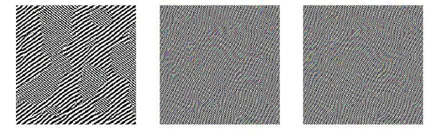
(a) Example of UAPs constructed by (Khrulkov and Oseledets 2018) (b) Turing patterns
Figure 1: Visual similarity of Universal Adversarial Perturbations by (Khrulkov and Oseledets 2018) and Turing patterns
Background to provide fast convergence:
Universal Adversarial Perturbations ψp0 (JTi (Xb )ψq (Ji (Xb )εt ))
εt+1 = , (4)
Adversarial perturbations are small disturbances added to kψp0 (JTi (Xb )ψq (Ji (Xb )εt ))kp
the inputs that cause machine learning models to make a where p10 + p1 = 1 and ψr (z) = sign(z)|z|r−1 , and Ji (Xb ) ∈
mistake. In (Szegedy et al. 2013) authors discovered these
noises by solving the optimization problem: Rbdi ×d for a batch Xb with batch size b is given as a block
matrix:
min kεk2 s.t. C(x + ε) 6= C(x), (1) Ji (x1 )
ε
Ji (Xb ) = ... . (5)
where x is an input object and C(·) is a neural network clas-
Ji (xb )
sifier. It was shown that the solution to the minimization
model (1) leads to perturbations imperceptible to human eye. For the case of p = ∞ (4) takes the form:
Universal adversarial perturbation (Moosavi-Dezfooli εt+1 = sign(JTi (Xb )ψq (Ji (Xb )εt )). (6)
et al. 2017) is a small (kεkp ≤ L) noise that makes clas-
sifier to misclassify the fraction (1 − δ) of inputs from the Equation (6) is the first crucial point in our study, and we
given dataset µ. The goal is to make δ as small as possible will show, how they connect to Turing patterns. We now
and find a perturbation ε such that: proceed with describing the background behind these pat-
terns and mathematical correspondence between Equation
Px∼µ [C(x + ε) 6= C(x)] ≥ 1 − δ s.t. kεkp ≤ L, (2) (6) and emergence of Turing patterns as cellular automata is
described in next Section.
In (Khrulkov and Oseledets 2018) an efficient way of
computing such UAPs was proposed, achieving relatively Turing Patterns as Cellular Automata
high fooling rates using only small number of inputs. Con- In his seminal work (Turing 1952) Alan Turing studied the
sider an input x ∈ Rd , its i-th layer output fi (x) ∈ Rdi and emergence theory of patterns in nature such as stripes and
∂fi (x)
Jacobian matrix Ji (x) = ∂x ∈ Rdi ×d . For a small in- spots that can arise out of a homogeneous uniform state.
x The proposed model was based on the solution of reaction-
put perturbation ε ∈ Rd , using first-order Taylor expansion diffusion equations of two chemical morphogens (reagents):
fi (x + ε) ≈ fi (x) + Ji (x)ε, authors find that to construct
a UAP, it is sufficient to maximize the sum of norms of Ja- ∂n1 (i, j)
= −µ1 ∇2 n1 (i, j) + a(n1 (i, j), n2 (i, j)),
cobian matrix product with perturbation for a small batch of ∂t (7)
inputs Xb , constrained with perturbation norm (kεkp = L is ∂n2 (i, j) 2
obtained by multiplying the solution by L): = −µ2 ∇ n2 (i, j) + b(n1 (i, j), n2 (i, j)).
∂t
X Here, n1 (i, j) and n2 (i, j) are concentrations of two
kJi (xj )εkqq → max, s.t. kεkp = 1. (3)
morphogens in the point with coordinates (i, j) µ1 and
xj ∈Xb
µ2 are scalar coefficients. a and b are nonlinear func-
To solve the optimization problem (3) the Boyd iteration tions, with at least two points (i, j), satisfying (i, j) :
(Boyd 1974) (generalization of the power method to the a(n1 (i, j), n2 (i, j)) = 0
problem of computing generalized singular vectors) is found b(n1 (i, j), n2 (i, j)) = 0.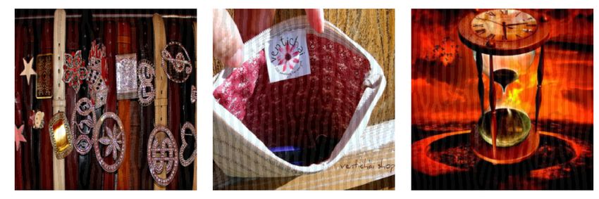
Turing noted the solution presents alternating patterns where Dj (x) = diag(θ(Mj fj−1 (x))) ∈ Rdj ×dj and
with specific size that does not depend on the coordinate
1, if z > 0
and describes the stationary solution, which interpolates be- θ(z) = ∂ ReLU(z)
∂z = .
0, if z < 0,
tween zeros of a and b.
The update matrix from Equation (13) is then:
Young et. al (Young 1984) proposed to generate Turing
patterns by a discrete cellular automata as following. Let us
Ji (x1 )
consider a 2D grid of cells. Each cell (i, j) is equipped with
JTi (Xb )Ji (Xb ) = JTi (x1 ) · · · JTi (xb ) ... =
a number n(i, j) ∈ {0, 1}. The sum of cells, neighbouring
with the current cell (i, j) within the radius ri is multiplied Ji (xb )
by w, while the sum of values of cells, neighbouring with the X
current cell (i, j) between radii rin and rout , is multiplied = JTi (x)Ji (x). (16)
by −1. If the total sum of these two terms is positive, the x∈Xb
new value of the cell is 1, otherwise 0. This process can be Performance of the UAPs from (Khrulkov and Oseledets
written by introducing the convolutional kernel Y (m, l): 2018) increases with the increase of batch size. Then consid-
w if |m|2 + |l|2 < rin
2
, ering the limit case of sufficiently large batch size b we can
Y (m, l) = 2 2 2 2 (8) approximate the averaging in (16) by the expected value:
−1 if rout > |m| + |l| > rin . P T
The coefficient w is found from the condition that the sum Ji (x)Ji (x)
x∈Xb
≈ Ex JTi (x)Ji (x) =
of elements of kernel Y is set to be 0:
XX b
Y (m, l) = 0. (9) = E MT1 DT1 (x) · · · MTi DTi (x)Di (x)Mi · · · D1 (x)M1 .
m l (17)
The update rule is written as: Note that DTj (x)Dj (x) = D2j (x) = DTj (x) = Dj (x). To
1 simplify Equation (17), we make additional assumption.
nk+1 (i, j) = [sign (Y ? nk (i, j)) + 1] , (10) Assumption 0. The elements of the diagonal matrices Dj
2
have the same scalar mean value cj :
where ? denotes a usual 2D convolution operator:
XX Ex [Dj (x)] ≈ cj I. (18)
Y ? n(i, j) = Y (m, l)n(i + m, j + l). (11)
m l This is based on the fact that we consider universal at-
tack, which is input-independent, we can assume x as ran-
For convenience, instead of {0, 1}, we can use ±1 and dom variable and D(x) as random matrix, which is diagonal
rewrite (10) (considering condition (9)) as: and have elements 0 or 1. Then our assumption is not unre-
nk+1 (i, j) = sign Y ? nk (i, j) . (12) alistic, as we assume that all diagonal elements of random
diagonal matrix over expectation converge to the same num-
Note that (12) is similar to (6), and lets investigate this con- ber c between 0 and 1 (see Appendix). Then, taking into
nection in more details. consideration (16), (17), (18) for the first layer:
JT1 (Xb )J1 (Xb ) ≈ bEx MT1 DT1 (x)D1 (x)M1 =
Connection between Boyd iteration and
Cellular Automata = bMT1 Ex [D1 (x)] M1 = bc1 MT1 M1 , (19)
We restrict our study to the case q = 2. Then ψ2 (z) = z and i.e. taking the expected value has removed the term corre-
Equation (6) can be rewritten as: sponding to the non-linearity!
εt+1 = sign(JTi (Xb )Ji (Xb )εt ). (13) Two subsequent convolutions does not result into one con-
volution, however the only source of error is boundary ef-
In (Khrulkov and Oseledets 2018) it was shown that per- fects. Since the size of convolutional kernels d < 10 is much
turbations of the first layers give the most promising results. smaller than the dimension of image N = 224 (for Ima-
Initial layers of most of the state-of-the-art image classifica- genet), the error is small and is up to d/N ≈ 0.5 ∗ 10−2 .
tion neural networks are convolutional followed by nonlin- It definetely could be neglected for our purposes. Moreover,
ear activation functions σ (e.g. ReLU(z) = max(0, z)). If as shown in (Miyato et al. 2018), this is common in convo-
the network does not include other operations (such as pool- lutional neural networks for images. One can advocate this
ing or skip connections) the output of the i-th layer is: by the asymptotic theory of Toeplitz matrices (Böttcher and
fi (x) = σ(Mi fi−1 (x)), (14) Grudsky 2000). Thus, we have shown that JT1 (Xb )J1 (Xb )
where Mi ∈ R di ×di−1
is a matrix of the 2D convolution has an approximate convolutional structure. To show that
operator of the i-th layer, corresponding to the convolutional JTi (Xb )Ji (Xb ) is also convolutional, we introduce addi-
kernel Ki .Using chain rule, the Jacobian in (6) is: tional assumptions:
Assumption 1. Matrices Dj (x) and Dk (x) are indepen-
∂fi (x) ∂f1 (x) dent for all pairs of j and k. In practice we only will check
Ji (x) = ··· = Di (x)Mi · · · D1 (x)M1 ,
∂fi−1 (x) ∂x the uncorrelation instead of independency, these checks are
(15) reported in appendix.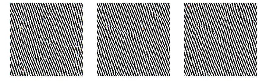
Figure 2: UAPs for different layers of VGG-19 classifier. According to the theory, the specific feature size of the patterns
increases with the depth of the attacked layer. The numbering of images is row-wise. First row corresponds to Layers 1-5,
second row - Layers 6-10, third row - Layers 11-15.
Assumption 2. Diagonal elements dj = θ(Mj fj−1 (x)) of Theorem 0.1 Given x is a random variable, A = A(x)
matrix Dj (x) have covariance matrix of convolutional struc- is a square matrix, such that Ex [A] = B is convolu-
ture Cj as linear operators of typical convolutional layers: tional, and D = D(x) is a diagonal matrix, such that
Ex [Dll Dmm ] = Clm and matrices D and A are indepen-
Cov(dj , dj ) = Cj . (20) dent. Then, Ex [DAD] is a convolutional matrix.
These two assumptions might seem to be strong, so here we Proof:
discuss how realistic and legit they are.
Regarding assumption 1, we should point that matrix D is Ex [DAD(x)]lm = Ex [Dll Alm Dmm ] =
not the outputs of ReLU activation function, but is indicator = Ex [Alm ] Ex [Dll Dmm ] = Blm Clm = (B ◦ C)lm ,
(0 and 1) whether the feature is positive or negative, and this
is reasonable to assume the independence between elements where ◦ denotes element-wise product.
Di and Dj . Further, let us consider covariaance of matrix Applying Theorem 0.1 for each of the layers, and using
elements of diagonal matrices Cov(Di , Dj ). First of all, for Dj = Dj (x) for all j in (16) and (17):
a large enough image batch it is natural to assume that this
JTi (Xb )Ji (Xb ) =
covariance if translationally invariant, i.e there is no selected
no correlation with D1
points. This means Cov(Dp,q l,m
i , Di ) = Ci (p − l, q − m) z }| {
which is nothing but the assumption 2. It is also follows that = bE MT1 DT1 · · · MTi DTi Di Mi · · · D1 M1 =
because of finite receptive field, convolution matrix Ci is
decreasing far from the diagonal.
These assumptions need additional conditions for satis- = bMTi ((· · · MT2 ((MT1 C1 M1 ) ◦ C2 )M2 · · · ) ◦ Ci )Mi ,
factory boundary effects, however we find them natural, and (21)
realistic to hold in the main part of features. Additional
quantitative experimental justifications of these assumptions which concludes that matrix JTi (Xb )Ji (Xb ) is convolu-
are in the Appendix. tional matrix and Boyd algorithm (6) indeed generates cel-
lular automata (12).(a) MobileNetV2 (b) VGG-19 (c) InceptionV3
Figure 3: Turing patterns generated using simplest kernels, parameterized by two numbers l1, l2.
Target Random Optimized Target model With Without
MobileNetV2 52.79 56.15
250 q 500 q 250 q 500 q
VGG-19 52.56 55.4
MobileNetV2 85.62 90.91 91.67 94.47
InceptionV3 45.32 47.18 VGG-19 79.73 75.9 76.94 77.61
InceptionV3 52.9 54.2 53.71 53.23
Table 1: FRs of a random Turing pattern and the one opti-
mized in l1 , l2 and initialization. Even random Turing pat-
terns provide competitive results, proving high universality Table 2: FRs of patterns with and without optimization on
of this attack. Better optimizations are in the tables 6,7. initialization (250 and 500 queries)
As described earlier, complex Turing patterns can be
The structure of patterns by (Khrulkov and Oseledets
modeled with only several parameters. In order to test the
2018) contains some interesting elements, which has spe-
performance of Turing patterns as black-box UAPs for a spe-
cific size. We empirically find that changing the train batch
cific network, we learn this parameters in a black-box sce-
does not affect much neither form of pattern, nor its fooling
nario by maximizing the fooling rate, without accessing the
rate (Equation (22)), even if we use batch of white images.
model’s architecture. For a classifier f and N images, the
This supports the idea that the update matrix JTi (Xb )Ji (Xb )
fooling rate of Turing pattern ε(θ) with parameters θ is:
does not depend much on batch Xb , and can be replaced
with constant convolutional matrix by Equation (21). Based N
P
on Equation (21), we see that deeper the layer i we apply al- [arg max f (xi ) 6= arg max f (xi + ε(θ))]
i=1
gorithm in Equation (6) the more convolutions are involved. FR = . (22)
As it was mentioned in Section Turing patterns present al- N
ternating patterns with specific characteristic size. Based on There are several options how to parametrize CA, and
this intuition, we hypothesize that the specific size of the pat- we discuss them one-by-one. For all approaches the target
terns generated by (Khrulkov and Oseledets 2018) increases function is optimized on 512 random images from ImageNet
with the depth of the attacked layer for which UAP is con- (Russakovsky et al. 2015) train dataset, and perturbation is
structed. To ensure this, we consider VGG-19 (Simonyan constrained as kεk∞ ≤ 10. Following (Meunier, Atif, and
and Zisserman 2014) network. Initial layers of this network Teytaud 2019), we used evolutionary algorithm CMA-ES
are convolutional with ReLU activation. We apply algorithm (Hansen, Müller, and Koumoutsakos 2003) by Nevergrad
to each of the first 15 layers of the network. We chose q = 2 (Rapin and Teytaud 2018) as a black-box optimization al-
in Equation (6). As illustrated in Figure 2, the typical feature gorithm. Fooling rates are calculated for 10000 Imagenet
size of the patterns increases with the “depth of the attack”. validation images for torchvision pretrained models(VGG-
19 (Simonyan and Zisserman 2014), InceptionV3 (Szegedy
Turing Patterns as Black-box Universal et al. 2016), MobilenetV2 (Sandler et al. 2018)).
Simple CA. Here, we fix the kernel Y in Equation (12)
Adversarial Perturbations to be L × L (we find that L = 13 produces best results),
The connection in the previous section suggests the use of with elements filled by −1, except for the inner central rect-
Turing patterns to craft UAPs in a black-box setting, learning angle of size l1 × l2 with constant elements such that the
parameters of CA by directly maximizing the fooling rate. sum of all elements of Y is 0. Besides l1 and l2 , the ini-(a) MobileNetV2 (b) VGG-19 (c) InceptionV3
Figure 4: Turing patterns generated using optimization on initialization and convolutional kernel Y
aa aa
Threshold Threshold
a a max max − 1 0.9 ∗ max a a max max − 1 0.9 ∗ max
Mixing aa Mixing aa
a a
Summation 77.5 78.0 77.9 Summation 53.1 50.6 51.0
Pointwise 78.0 77.7 78.0 Pointwise 53.3 53.6 53.5
Table 3: Experiments with DFT frequencies for VGG-19 Table 4: Experiments with DFT frequencies for InceptionV3
tialization of n(i, j) from Eq. (12) is added as parameters.
To reduce black-box queries, initialization is chosen to be
7 × 7 square tiles (size 32 × 32) (Meunier, Atif, and Tey-
taud 2019) for each of the 3 maps representing each image
channel. θ = (l1 , l2 , initialization). Resulting UAPs
are shown in Fig. 3. Improvement over the random Turing
pattern (with random, not optimized parameters) is shown in (b) Optimization over kernel
Table 1 and full results are in Table 5. We should point, here, (a) Optimization over kernel and only, averaged over 10 initializa-
initialization maps tions (min and max highlighted)
our method is black-box, i.e. without access to the architec-
ture and weights, and we do not compare it to (Khrulkov and
Oseledets 2018) as they consider white-box scenario with Figure 5: Pattern fooling rate (vertical axis) dependence on
full access to the network. Moreover, even if we consider the kernel size (horizontal axis). This figure shows that there
black-box scenario, our results using more advanced opti- is no dependence on the kernel size.
mization are significantly better in terms of fooling rate (see
Tables 6-7) even comparing to the white-box.
CA with kernel optimization. In this scenario, all ele- Another resource for optimization are different strategies
ments of the kernel Y are considered as unknown parame- for dealing with the channels of the image (This might pro-
ters. Optimizing both over Y and the initialization maps we duce color patches). The detailed experiments are given in
got a substantial increase in fooling rates (see Fig. 4 for per- the Appendix, the results for the best case are in Table 7.
turbations and Table 6 for fooling rate results). Results for
different kernel sizes are shown in Fig. 5a. Similarity to Fourier attacks
Optimization with random initialization map. Here, Some of the patterns are similar to the ones generated as
we remove the initialization map from the optimized param- single Fourier harmonics, in (Tsuzuku and Sato 2019). To
eters select it randomly. As experiments show (see Table 2), compare correspondence, we took the discrete Fourier trans-
the performance of patterns generated without optimized ini- form (DFT) of the pattern and cut all the frequencies with
tialization maps does not differ significantly from the pattern the amplitude below some threshold (we used 2 cases of
with optimized initialization maps. Thus, the initialization thresholds: max −1 and 0.9 max) and then reversed the DFT
maps for pattern generation can be randomly initialized, and for all three pattern channels. We applied this transforma-
less queries can be made without significant loss in fooling tion to the patterns acquired using different channel mix-
rates. Results for different kernel sizes are shown in Fig. 5b. ing approaches (2 (summation) and 4 (pointwise) describedaa
aa Target ResNet GoogleNet VGG-16
MobileNetV2 VGG-19 InceptionV3 SFA 40.1 44.1 53.3
Trained on
aa
aa Ours 61.4 58.2 81.2
MobileNetV2 56.15 56.96 45.16
VGG-19 50.49 55.4 49.98 Table 8: Performance of Turing Patterns (2 parameters)
InceptionV3 49.55 48.76 47.18 and SFA: Single Fourier Attack (Tsuzuku and Sato 2019)
(224*224*3 parameters) in a black-box scenario
Table 5: Optimization on l1 , l2 , and initialization
aa tors to perturb hidden layers. Tsuzuku et al. (Tsuzuku and
aa Target
MobileNetV2 VGG-19 InceptionV3 Sato 2019) used Fourier harmonics of convolutional layers
Trained on
aa
aa without any activation function. Though UAPs were first
MobileNetV2 90.59 61.27 35.15 found in image classification, they exist in other areas as
VGG-19 62.15 75.64 31.91 well, such as semantic segmentation (Metzen et al. 2017),
InceptionV3 65.69 76.40 53.93 text classifiers (Behjati et al. 2019), speech and audio recog-
nition (Abdoli et al. 2019; Neekhara et al. 2019).
Table 6: Optimization on kernel Y and initialization Turing Patterns. Initially introduced by Alan Turing in
(Turing 1952), Turing patterns have attracted a lot of at-
aa tention in pattern formation studies. Patterns like fronts,
aa Target
MobileNetV2 VGG-19 InceptionV3 hexagons, spirals and stripes are found as a result of Tur-
Trained on
aa
aa ing reaction–diffusion equations (Kondo and Miura 2010).
MobileNetV2 94.78 57.90 35.04 In nature, Turing patterns has served as a model of fish
VGG-19 73.15 77.50 43.06 skin pigmentation (Nakamasu et al. 2009), leopard skin pat-
InceptionV3 63.90 64.46 53.10 terns (Liu, Liaw, and Maini 2006), seashell patterns (Fowler,
Meinhardt, and Prusinkiewicz 1992). Interesting to Neuro-
Table 7: Summation channel mixing science community, might be connection of Turing patterns
to brain (Cartwright 2002; Lefèvre and Mangin 2010).
Cellular Automata in Deep Learning. Relations be-
above). As a result, in most cases neither the fooling rates tween Neural Networks and Cellular Automata were discov-
(see Table 3, 4) nor the visual representation of the pattern ered in several works (Wulff and Hertz 1993; Gilpin 2019;
(Appendix, Fig. 6) did not change drastically, which leads Mordvintsev et al. 2020). Cellular automaton dynamics with
us to the conclusion that in these cases it is indeed a Sin- neural network was studied in (Wulff and Hertz 1993). In
gle Fourier Attack that is taking place. However, in the case (Gilpin 2019) authors generate cellular automata as convo-
of patterns generated using summation channel mixing to lutional neural network. In (Mordvintsev et al. 2020) it was
attack InceptionV3 it is not true (Appendix, Fig. 7). This shown that training cellular automata using neural networks
means that while such methods can generate Single Fourier can organize cells into shapes of complex structure.
Attacks, not all the attacks generated using these methods
are SFA, i.e. our approach can generate more diverse UAPs. Conclusion
Our work compared to (Tsuzuku and Sato 2019) has much The key technical point of our work is that a complicated Ja-
less parameters and performs better (see Table 8). cobian in the Boyd iteration can be replaced without sacrific-
ing the fooling rate by a single convolution, leading to a re-
Related Work markably simple low-parametric cellular automata that gen-
Adversarial Perturbations. Intriguing vulnerability of neu- erates universal adversarial perturbations. It also explains
ral networks in (Szegedy et al. 2013; Biggio et al. 2013) pro- the similarity between UAPs and Turing patterns. It means
posed numerous techniques to construct white-box (Good- that the non-linearities are effectively averaged out from the
fellow, Shlens, and Szegedy 2015; Carlini and Wagner 2017; process. This idea could be potentially useful for other prob-
Moosavi-Dezfooli, Fawzi, and Frossard 2016; Madry et al. lems involving the Jacobians of the loss functions for com-
2017) and black-box (Papernot et al. 2017; Brendel, Rauber, plicated neural networks, e.g. spectral normalization.
and Bethge 2017; Chen and Pock 2017; Ilyas et al. 2018) ad- This work studies theory of interesting phenomena of
versarial examples. Modern countermeasures against adver- Universal Adversarial Perturbations. Fundamental suscepti-
sarial examples have been shown to be brittle (Athalye, Car- bility of deep CNNs to small alternating patterns, that are
lini, and Wagner 2018). Interestingly, input-agnostic Uni- easily generated, added to images was shown in this work
versal Adversarial Perturbations were discovered recently and their connection to Turing patterns, a rigorous theory in
(Moosavi-Dezfooli et al. 2017). Several methods were pro- mathematical biology that describes many natural patterns.
posed to craft UAPs (Khrulkov and Oseledets 2018; Mop- This might help to understand the theory of adversarial per-
uri, Garg, and Babu 2017; Tsuzuku and Sato 2019). Mop- turbations, and in the future to robustly defend from them.
uri et al. (Mopuri, Garg, and Babu 2017) used activation-
maximization approach. Khrulkov et al. (Khrulkov and Os- Acknowlegements
eledets 2018) proposed efficient use of (p, q)−singular vec- This work was supported by RBRF grant 18-31-20069.References Khrulkov, V.; and Oseledets, I. 2018. Art of singular vec-
Abdoli, S.; Hafemann, L. G.; Rony, J.; Ayed, I. B.; Cardinal, tors and universal adversarial perturbations. In Proceedings
P.; and Koerich, A. L. 2019. Universal adversarial audio of the IEEE Conference on Computer Vision and Pattern
perturbations. arXiv preprint arXiv:1908.03173 . Recognition, 8562–8570.
Athalye, A.; Carlini, N.; and Wagner, D. 2018. Obfus- Kondo, S.; and Miura, T. 2010. Reaction-diffusion model as
cated gradients give a false sense of security: Circum- a framework for understanding biological pattern formation.
venting defenses to adversarial examples. arXiv preprint science 329(5999): 1616–1620.
arXiv:1802.00420 . Lefèvre, J.; and Mangin, J.-F. 2010. A reaction-diffusion
Behjati, M.; Moosavi-Dezfooli, S.-M.; Baghshah, M. S.; and model of human brain development. PLoS computational
Frossard, P. 2019. Universal adversarial attacks on text clas- biology 6(4): e1000749.
sifiers. In ICASSP 2019-2019 IEEE International Confer- Liu, R.; Liaw, S.; and Maini, P. 2006. Two-stage Turing
ence on Acoustics, Speech and Signal Processing (ICASSP), model for generating pigment patterns on the leopard and
7345–7349. IEEE. the jaguar. Physical review E 74(1): 011914.
Biggio, B.; Corona, I.; Maiorca, D.; Nelson, B.; Šrndić, N.;
Madry, A.; Makelov, A.; Schmidt, L.; Tsipras, D.; and
Laskov, P.; Giacinto, G.; and Roli, F. 2013. Evasion attacks
Vladu, A. 2017. Towards deep learning models resistant to
against machine learning at test time. In Joint European
adversarial attacks. arXiv preprint arXiv:1706.06083 .
conference on machine learning and knowledge discovery
in databases, 387–402. Springer. Metzen, J. H.; Kumar, M. C.; Brox, T.; and Fischer, V. 2017.
Böttcher, A.; and Grudsky, S. M. 2000. Toeplitz matri- Universal adversarial perturbations against semantic image
ces, asymptotic linear algebra and functional analysis, vol- segmentation. In 2017 IEEE International Conference on
ume 67. Springer. Computer Vision (ICCV), 2774–2783. IEEE.
Boyd, D. W. 1974. The power method for lp norms. Linear Meunier, L.; Atif, J.; and Teytaud, O. 2019. Yet another
Algebra and its Applications 9: 95–101. but more efficient black-box adversarial attack: tiling and
evolution strategies. arXiv preprint arXiv:1910.02244 .
Brendel, W.; Rauber, J.; and Bethge, M. 2017. Decision-
based adversarial attacks: Reliable attacks against black-box Miyato, T.; Kataoka, T.; Koyama, M.; and Yoshida, Y. 2018.
machine learning models. arXiv preprint arXiv:1712.04248 Spectral normalization for generative adversarial networks.
. arXiv preprint arXiv:1802.05957 .
Carlini, N.; and Wagner, D. 2017. Towards evaluating the Moosavi-Dezfooli, S.-M.; Fawzi, A.; Fawzi, O.; and
robustness of neural networks. In 2017 IEEE Symposium on Frossard, P. 2017. Universal adversarial perturbations. In
Security and Privacy (SP), 39–57. IEEE. Proceedings of the IEEE conference on computer vision and
pattern recognition, 1765–1773.
Cartwright, J. H. 2002. Labyrinthine Turing pattern forma-
tion in the cerebral cortex. arXiv preprint nlin/0211001 . Moosavi-Dezfooli, S.-M.; Fawzi, A.; and Frossard, P. 2016.
Deepfool: a simple and accurate method to fool deep neural
Chen, Y.; and Pock, T. 2017. Trainable nonlinear reaction
networks. In Proceedings of the IEEE conference on com-
diffusion: A flexible framework for fast and effective image
puter vision and pattern recognition, 2574–2582.
restoration. IEEE transactions on pattern analysis and ma-
chine intelligence 39(6): 1256–1272. Mopuri, K. R.; Garg, U.; and Babu, R. V. 2017. Fast feature
Fowler, D. R.; Meinhardt, H.; and Prusinkiewicz, P. 1992. fool: A data independent approach to universal adversarial
Modeling seashells. In Proceedings of the 19th annual con- perturbations. arXiv preprint arXiv:1707.05572 .
ference on Computer graphics and interactive techniques, Mordvintsev, A.; Randazzo, E.; Niklasson, E.; and Levin, M.
379–387. 2020. Growing neural cellular automata. Distill 5(2): e23.
Gilpin, W. 2019. Cellular automata as convolutional neural Nakamasu, A.; Takahashi, G.; Kanbe, A.; and Kondo, S.
networks. Physical Review E 100(3): 032402. 2009. Interactions between zebrafish pigment cells respon-
Goodfellow, I.; Shlens, J.; and Szegedy, C. 2015. Ex- sible for the generation of Turing patterns. Proceedings of
plaining and Harnessing Adversarial Examples. In Inter- the National Academy of Sciences 106(21): 8429–8434.
national Conference on Learning Representations. URL Neekhara, P.; Hussain, S.; Pandey, P.; Dubnov, S.; McAuley,
http://arxiv.org/abs/1412.6572. J.; and Koushanfar, F. 2019. Universal adversarial per-
Hansen, N.; Müller, S. D.; and Koumoutsakos, P. 2003. Re- turbations for speech recognition systems. arXiv preprint
ducing the time complexity of the derandomized evolution arXiv:1905.03828 .
strategy with covariance matrix adaptation (CMA-ES). Evo- Papernot, N.; McDaniel, P.; Goodfellow, I.; Jha, S.; Celik,
lutionary computation 11(1): 1–18. Z. B.; and Swami, A. 2017. Practical black-box attacks
Ilyas, A.; Engstrom, L.; Athalye, A.; and Lin, J. 2018. against machine learning. In Proceedings of the 2017 ACM
Black-box adversarial attacks with limited queries and in- on Asia conference on computer and communications secu-
formation. arXiv preprint arXiv:1804.08598 . rity, 506–519.Rapin, J.; and Teytaud, O. 2018. Nevergrad-A gradient- free optimization platform. version 0.2. 0, https://GitHub. com/FacebookResearch/Nevergrad . Russakovsky, O.; Deng, J.; Su, H.; Krause, J.; Satheesh, S.; Ma, S.; Huang, Z.; Karpathy, A.; Khosla, A.; Bernstein, M.; et al. 2015. Imagenet large scale visual recognition chal- lenge. International journal of computer vision 115(3): 211– 252. Sandler, M.; Howard, A.; Zhu, M.; Zhmoginov, A.; and Chen, L.-C. 2018. Mobilenetv2: Inverted residuals and lin- ear bottlenecks. In Proceedings of the IEEE conference on computer vision and pattern recognition, 4510–4520. Simonyan, K.; and Zisserman, A. 2014. Very deep convo- lutional networks for large-scale image recognition. arXiv preprint arXiv:1409.1556 . Szegedy, C.; Vanhoucke, V.; Ioffe, S.; Shlens, J.; and Wojna, Z. 2016. Rethinking the inception architecture for computer vision. In Proceedings of the IEEE conference on computer vision and pattern recognition, 2818–2826. Szegedy, C.; Zaremba, W.; Sutskever, I.; Bruna, J.; Erhan, D.; Goodfellow, I.; and Fergus, R. 2013. Intriguing prop- erties of neural networks. arXiv preprint arXiv:1312.6199 . Tsuzuku, Y.; and Sato, I. 2019. On the Structural Sensitivity of Deep Convolutional Networks to the Directions of Fourier Basis Functions. In Proceedings of the IEEE Conference on Computer Vision and Pattern Recognition, 51–60. Turing, A. M. 1952. The chemical basis of morphogenesis. Bulletin of mathematical biology 52(1-2): 153–197. Wulff, N.; and Hertz, J. A. 1993. Learning cellular automa- ton dynamics with neural networks. In Advances in Neural Information Processing Systems, 631–638. Young, D. A. 1984. A local activator-inhibitor model of ver- tebrate skin patterns. Mathematical Biosciences 72(1): 51– 58.
Appendix                                       aa
                                                                   aa          Channel
                                                                  Target  aamixing Independent           Summation      3D filter   Pointwise
     Numerical justification of assumptions                       model       aa
To experimentally bolster our assumptions we made follow-         MobileNetV2
                                                                                 a
                                                                                      60.87                 94.78        81.97       94.26
ing experiments:                                                  VGG-19              60.74                 77.50        78.87       78.00
 • Assumption 0                                                   InceptionV3         47.45                 53.10        51.31       53.33
   To justify equation 18 we calculated the average value
   and the standard deviations of diagonal matrices Di corre-    Table 11: Fooling rates for different channel mixing ap-
   sponding to ReLU layers (see Figure 8) results are shown      proaches
   in Table 9. We assume that Assumption 0 holds, by show-
   ing small coefficients of variations for mean values of di-
   agonal elements of the matrices.                              We compared the following approaches to mixing channel
                                                                 maps during pattern generation:
 Matrix (Di )    Mean value E[Di ]     Variation (std/mean)       • One 2D-filter for all 3 independent image channels, no
    D1           0.6530 ± 0.0621                9.5%                channel mixing
    D2           0.4267 ± 0.0362               8.48%              • One 2D-filter for all image channels, after convolution the
    D3           0.4288 ± 0.0663              15.46%                sum of each two channels becomes the remaining channel
    D4            0.309 ± 0.0401              12.97%                (i.e. channel3 = channel1 + channel2)
    D5           0.3552 ± 0.0515              14.49%              • One 3D-filter for all 3 image channels
    D6           0.3316 ± 0.0578             0.1743%
                                                                  • 3 separate 2D-filters (one for each channel), and a 3 × 3
            Table 9: Assumption 0 experiments                       matrix for channel mixing, like pointwise convolution
                                                                 One can expect for 3D-filter to be a generalization of all of
                                                                 the other cases, thus it would be the most optimal to optimize
• Assumption 1 We also conduct some experiments to               over. However, as can be seen in Table 11, the results suggest
  check the Assumption 1, the most correlated elements are       that it is not definitevely better than the other approaches. It
  the corresponding elements of matrices Di and Dj , corre-      can be seen summation, 3D and pointwise approaches give
  sponding to i-th and j-th ReLU layers (see Figure 8). To       similar results, with pointwise performing slightly better on
  experimentally test this, we considered two binary vectors     average over the other models.
  (diagonals of matrices). We computed Simple Matching
  Coefficient (SMC, number of bit matches) between these         Transferability
  vectors for each of an image, and averaged over the whole
                                                                 We tested several patterns discussed earlier for their trans-
  validation dataset. ISMC shows what fraction of bits are
                                                                 ferability among the target networks. The results can be
  identical in two binary vectors. SMC=1 means total cor-
                                                                 seen in Table ??. It seems that the attacks generally trans-
  relation. SMC=0 means total negative correlation, while
                                                                 fer rather well to MobileNetV2 anf VGG-19, while Incep-
  SMC=0.5 means two vectors are uncorrelated and random
                                                                 tionV3 seems harder to transfer this types of attacks to. The
  to each other. The results are shown in Table 10.
                                                                 results show that while optimization over cellular automata
              Matrices      E[SM C(Di , Dj )]                    parameters seems to significantly boost fooling rates for
                                                                 target networks, some transferability loss can be expected.
             D1 and D2          0.4825                           Note that for MobileNetV2 we get almost 95% fooling rate.
             D3 and D4          0.5183
             D5 and D6          0.5528
             D6 and D7          0.5648                            Algorithm 1: (µw , λ)-CMA-ES algorithm
             D7 and D8          0.6096                             initialize < x >
                                                                   C ← I;
           Table 10: Assumption 1 experiments                      repeat
                                                                        B, D ← eigendecomposition(C)
                                                                        for i = 1 ← λ do
                                                                            yi ← B · D · N (0, I)
    Alternative methods of CA optimization                                  xi ←< x > +σyi
Effect of different filter sizes. Another experiment is the                 fi ← f (xi )
dependence of the fooling rate on the filter size. Here we              end
show results for both patterns with and without specifically                      Pµ
                                                                        < y >← i=1 wi yi:λ
optimized initialization maps (attacking MobileNetV2). In                                              Pµ
                                                                        < x >←< x > +σ < y >= i=1 wi xi:λ
both cases small filter size does not provide good results,             σ ← update(σ, C, y)
however surprisingly there is a non-monotonic dependence                C ← update(C, w, y)
on the filter sizes once they are larger than 7.                   until Termination criterion fulfilled;
   Effect of channel mixing. Different channel mixing
strategies within the pattern generation algorithm are used.
Figure 6: Pointwise channel mixing patterns attacking InceptionV3 after Fourier modification
Figure 7: Summation channel mixing patterns attacking InceptionV3 after Fourier modification
Figure 8: The architecture of VGG-19 (Simonyan and Zisserman 2014)
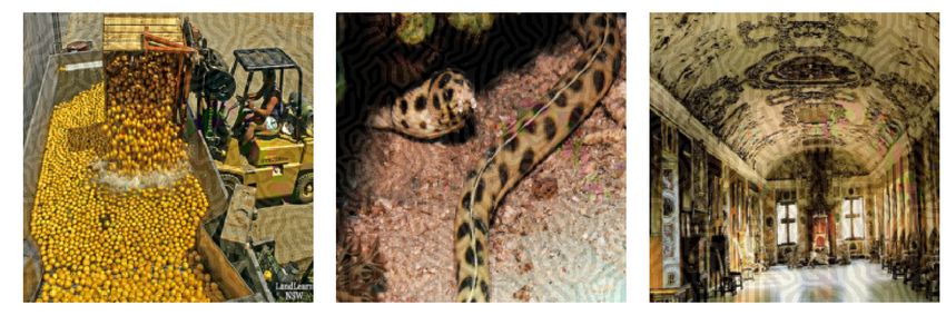
(a) Examples of images misclassified after the perturbation with (b) Examples of images misclassified after the perturbation with Tur-
UAPs from (Khrulkov and Oseledets 2018)( = 10) ing patterns ( = 10).
Figure 9: Examples of images misclassified after the perturbation with UAPs and Turing patterns.aa
aa Target
MobileNetV2 VGG-19 InceptionV3
Trained on
aa
aa
MobileNetV2 56.15 56.96 45.16
VGG-19 50.49 50.06 49.98
InceptionV3 49.55 48.76 47.18
Table 12: Turing patterns optimized in l1 , l2
aa
aa Target
MobileNetV2 VGG-19 InceptionV3
Trained on
aa
aa
MobileNetV2 90.59 61.27 35.15
VGG-19 62.15 75.64 31.91
InceptionV3 65.69 76.40 53.93
Table 13: Patterns optimized over filter Y and initialization maps
aa
aa Target
MobileNetV2 VGG-19 InceptionV3
Trained on
aa
aa
MobileNetV2 60.87 45.00 37.49
VGG-19 61.99 60.74 47.76
InceptionV3 53.22 54.54 47.45
Table 14: Independent channels
aa
aa Target
MobileNetV2 VGG-19 InceptionV3
Trained on
aa
aa
MobileNetV2 94.78 57.90 35.04
VGG-19 73.15 77.50 43.06
InceptionV3 63.90 64.46 53.10
Table 15: Summation channel mixing
aa
aa Target
MobileNetV2 VGG-19 InceptionV3
Trained on
aa
aa
MobileNetV2 81.97 68.30 48.24
VGG-19 76.15 78.87 43.83
InceptionV3 61.36 61.62 51.31
Table 16: 3D filter
aa
aa Target
MobileNetV2 VGG-19 InceptionV3
Trained on
aa
aa
MobileNetV2 94.26 57.80 35.05
VGG-19 74.79 78.00 43.38
InceptionV3 59.29 67.70 53.33
Table 17: Pointwise channel mixingYou can also read