Tide prediction machines at the Liverpool Tidal Institute - HGSS
←
→
Page content transcription
If your browser does not render page correctly, please read the page content below
Hist. Geo Space Sci., 11, 15–29, 2020
https://doi.org/10.5194/hgss-11-15-2020
© Author(s) 2020. This work is distributed under
the Creative Commons Attribution 4.0 License.

        Tide prediction machines at the Liverpool Tidal Institute
                                                    Philip L. Woodworth
          National Oceanography Centre, Joseph Proudman Building, 6 Brownlow Street, Liverpool, L3 5DA, UK
                                  Correspondence: Philip L. Woodworth (plw@noc.ac.uk)

           Received: September 2019 – Revised: 17 January 2020 – Accepted: 7 February 2020 – Published: 20 March 2020

       Abstract. The 100th anniversary of the Liverpool Tidal Institute (LTI) was celebrated during 2019. One aspect
       of tidal science for which the LTI acquired a worldwide reputation was the development and use of tide prediction
       machines (TPMs). The TPM was invented in the late 19th century, but most of them were made in the first half of
       the 20th century, up until the time that the advent of digital computers consigned them to museums. This paper
       describes the basic principles of a TPM, reviews how many were constructed around the world and discusses
       the method devised by Arthur Doodson at the LTI for the determination of harmonic tidal constants from tide
       gauge data. These constants were required in order to set up the TPMs for predicting the heights and times of
       the tides. Although only 3 of the 30-odd TPMs constructed were employed in operational tidal prediction at
       the LTI, Doodson was responsible for the design and oversight of the manufacture of several others. The paper
       demonstrates how the UK, and the LTI and Doodson in particular, played a central role in this area of tidal
       science.

1   Introduction                                                  graphic Laboratory. The LTI (as I shall continue to call it for
                                                                  the purpose of this paper) became an acknowledged centre
In the year following the end of the First World War, a num-      of expertise for research into ocean and earth tides, storm
ber of organisations were established which have had a last-      surges, sea level changes (Permanent Service for Mean Sea
ing importance for geophysical research. At an international      Level), and the measurement and modelling of coastal pro-
level, the International Union of Geodesy and Geophysics          cesses.
(IUGG) was founded in that year (Joselyn and Ismail-Zadeh,           Some of the history behind the establishment of the LTI is
2019). The 100th anniversary of the IUGG, which remains           described by Carlsson-Hyslop (2010, 2020). Short histories
the pre-eminent international body for geophysics, has been       may also be found in Doodson (1924) and Cartwright (1980,
marked by a series of papers in a special issue of this jour-     1999). The present paper focuses on one area of work for
nal (entitled “The International Union of Geodesy and Geo-        which the LTI became renowned, the development of tide
physics: from different spheres to a common globe”).              prediction machines (TPMs). Arthur Doodson (1890–1968)
   An example of an important development for geophysics          was the main person involved in this aspect of the LTI’s his-
at a national level was the establishment of the Liverpool        tory, and so he is the main character of interest for the present
Tidal Institute (LTI), marked by the set of papers in another     paper (Fig. 1a). Scoffield (2006) and Carlsson-Hyslop (2015)
special issue of this journal (entitled “Developments in the      contain details of his early career. Proudman (1968) provides
science and history of tides”). The LTI was based initially at    an excellent overview of many aspects of Doodson’s research
Liverpool University with Joseph Proudman as honorary di-         at the LTI, including that with the TPMs (see also Cartwright,
rector and Arthur Doodson as secretary. However, by 1929 it       1999).
had relocated across the river Mersey to Bidston Observatory         TPMs were analogue computers which, before the ad-
where there was more room for research and where Dood-            vent of digital computers, provided an accurate and efficient
son took up residence as associate director (Nature, 1928).       means of predicting the ocean tide, and in particular they pre-
It was renamed the Liverpool Observatory and Tidal Insti-         dicted the heights and times of high and low waters reported
tute, and during the next 100 years there were to be sev-         in tide tables. Cartwright (1999) gives a general explanation
eral other changes of name including the Proudman Oceano-

Published by Copernicus Publications.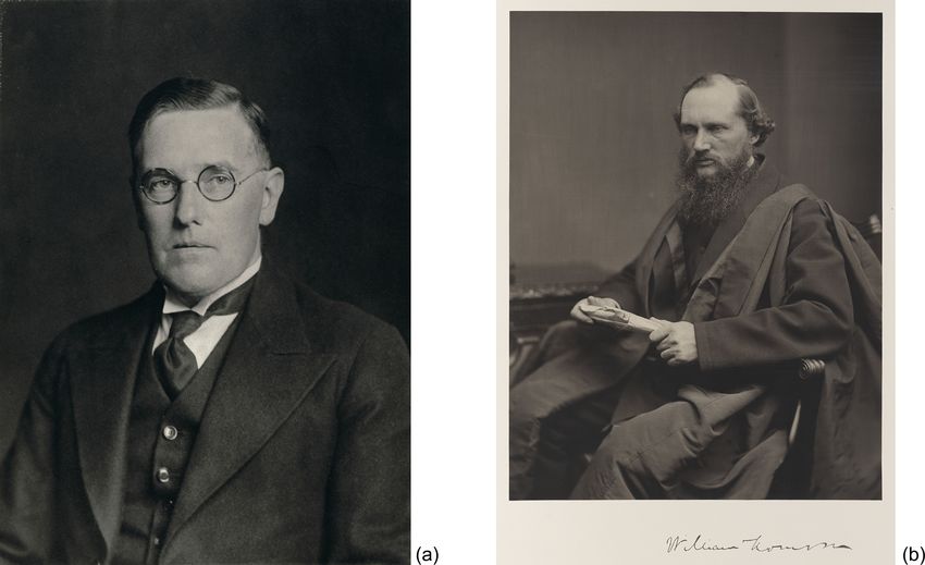
16 P. L. Woodworth: Tide prediction machines at the Liverpool Tidal Institute
lines of India and Australia. Another disadvantage of Lub-
bock’s method was that it required the use of long tide gauge
records, such as those from London or Liverpool (e.g. Lub-
bock, 1835). These deficiencies led to the development of
the harmonic method in the 1860s, first by Kelvin aided by
Roberts, and then also by Sir George Darwin (the second
son of Charles Darwin) and others, under the auspices of the
BAAS. The harmonic method’s advantage of being able to
use short tide gauge records (i.e. a year or less) ultimately
enabled tidal predictions to be produced for ports located in
any tidal regime.
Using the harmonic method, the tide at any one location
can be described with good accuracy as an expansion in
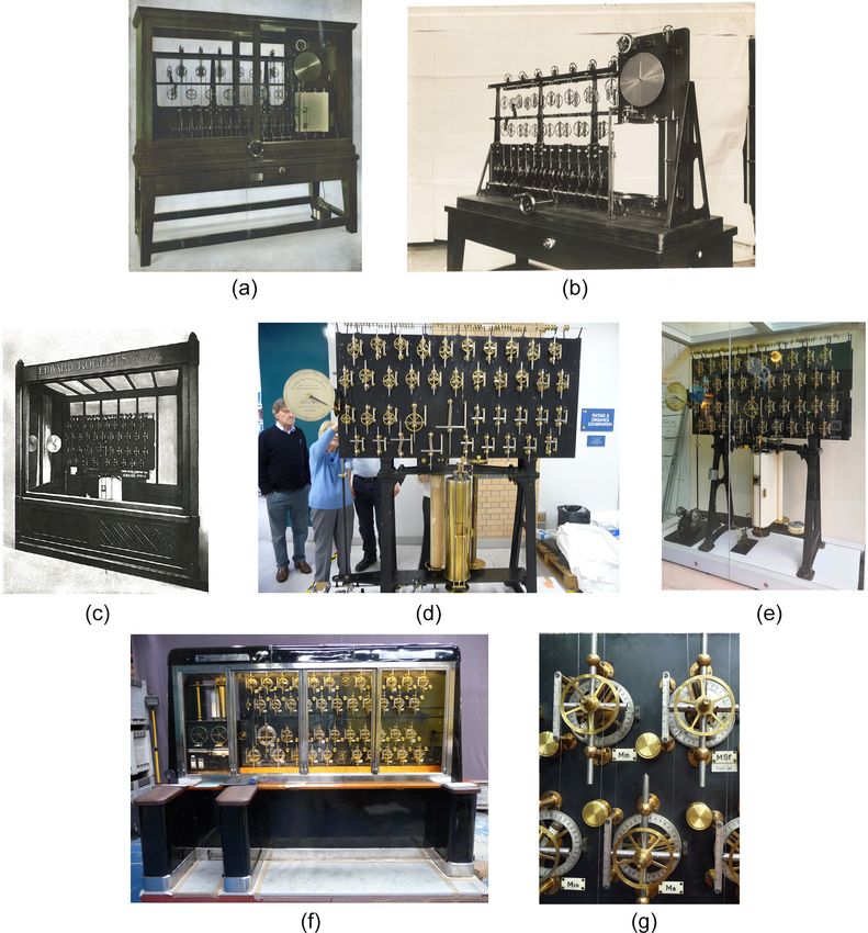
Figure 1. (a) Arthur Thomas Doodson CBE, DSc, FRS, terms of a number (N) of “constituents” or “satellites” such
FRSE (1890–1968) photographed in 1933 by Walter Stone- that
man. (b) Sir William Thomson (1st Baron Kelvin of Largs)
OM, GCVO, PC, FRS, FRSE (1824–1907) photographed in 1871 N
X
by Thomas Annan. © National Portrait Gallery, London. htotal (t) = hi cos (ωi t − gi ) , (1)
i=1
of TPMs and provides a description of some of them, while where the total tide htotal at time t is expressed as a sum of
Hughes (2005) contains some of the history of the individu- one cosine for each constituent; ωi is the angular speed of
als associated with them. constituent i; ωi = 2π
Ti , where Ti is its period; and hi and gi
The first TPM (aside from prototype models) was designed are its amplitude and phase lag. N is infinite in principle but,
by Sir William Thomson (1824–1907, Baron Kelvin of Largs in practice, the ocean tide can be described with good ac-
from 1892; Fig. 1b), with the help of Edward Roberts from curacy at most open-ocean locations by several 10 s of con-
the UK Nautical Almanac Office, and was constructed by the stituents.1
scientific equipment company of Alexander Légé in 1872– Consequently, if one has prior knowledge of each ωi , hi
1873 with funding from the British Association for the Ad- and gi , then one can calculate the height of the tide at any
vancement of Science (BAAS). Therefore, all TPMs are time t from the set of cosines. How one acquires this prior
sometimes referred to as “Kelvin machines”, although this knowledge will be explained below. The “turning points” of
name is also used to refer to a particular type of TPM (see the tidal curve (when ∂htotal /∂t = 0) will provide the heights
below). Between the 1870s and 1960s, over 30 TPMs were and times of high and low waters.
constructed around the world, of which the majority were One could undertake such a tedious arithmetic computa-
made in the UK. Only three of them were used for tidal pre- tion oneself, by calculating the height of the tide every hour
diction at the LTI. However, there were more for which Doo- during the year, by plotting the resulting time series and by
dson played a major role in their design. In addition, he su- inspecting the plot to see when the turning points occur and
pervised closely their manufacture by the Légé company and what their heights are. However, it was Kelvin’s realisation
provided a certificate of efficiency prior to delivery to cus- that TPMs could provide a means for undertaking such a
tomers. As a consequence, the LTI played the central role task more efficiently, their accuracy being limited only by
between the 1920s and 1960s in this area of tidal science. the number of constituents or “components” (N) included in
their design, that led to their development and use in tidal
2 The harmonic method
1 Equation (1) is shown in a simplified form, omitting astro-
Cartwright (1999) contains a comprehensive description of nomical arguments and nodal factors and with the mean level
the history of tidal science from antiquity to the present day. set to zero. It can be written more fully as htotal (t) = Z0 +
N
During most of the 19th century, tide tables in the UK were P
hi fi cos (ωi t − gi + (Vi + ui )), where Vi is called the astronom-
produced using the non-harmonic or “synthetic” method de- i=1
ical argument for constituent i at time t = 0 and the nodal factors
veloped by Sir John Lubbock (Baron Avebury) (Rossiter,
fi and ui are time-dependent adjustments to the amplitudes and
1971; Durand-Richard, 2016a). That method worked well in phase lags respectively of lunar tidal constituents (those for solar
areas with predominantly semidiurnal tides, and in fact the constituents are simply 1.0 and 0.0 respectively); V , f and u can
Admiralty continued to use non-harmonic methods derived all be computed readily using standard formulae which are derived
from Lubbock’s work well into the 20th century (Rossiter, from knowledge of the orbits of the sun and moon; and Z0 indicates
1971). However, it was less suitable in regions with pro- the mean level of the record. See Pugh and Woodworth (2014) for
portionately larger diurnal tides such as along the coast- more details.
Hist. Geo Space Sci., 11, 15–29, 2020 www.hist-geo-space-sci.net/11/15/2020/
P. L. Woodworth: Tide prediction machines at the Liverpool Tidal Institute                                                            17

prediction up until the 1960s.2 Kelvin’s first machine (the
so-called “British Association Machine”), derived from a de-
vice used in telegraphy by Sir Charles Wheatstone, could
simulate a tide containing 10 constituents. Later machines
included many more, as shown in Table 1a. The largest ac-
counted for 62 harmonic constituents. That is the enormous
machine, weighing 7 t, designed in Germany by Heinrich
Rauschelbach and now on display at the Deutsches Museum
in Munich (Cartwright, 1999). It is denoted as TPM-S16 in
Table 1a. Although open-ocean tides could be predicted ef-
fectively in this way, Doodson was always rightly sceptical
about the ability of TPMs to simulate tides in estuaries, even
when N was large (Doodson, 1926).                                      Figure 2. Schematic figure of a TPM based on drawings in Doo-
                                                                       dson and Warburg (1941). (a) A method for producing vertical si-
                                                                       nusoidal motion corresponding to that of one tidal constituent and
3   Schematic description of a TPM                                     (b) a method for summing six constituents with the use of a band
                                                                       wrapping around each pulley. See the text for further explanation.
Each TPM had its own architecture (as a modern computer
scientist might say). However, there were several features
common to almost all of them. First, one had to have a driv-           stituent in the machine has to be consistent with the phase
ing mechanism (either by hand or electric motor) to provide a          lag of that constituent in the real ocean tide. Many practical
circular motion with an angular frequency ωi corresponding             aspects involved in the construction of a working TPM are
to that of a tidal constituent. Second, one required a mecha-          described in chap. 14 of Doodson and Warburg (1941).
nism for converting that circular motion into sinusoidal mo-              Figure 2 is adapted from drawings in Doodson and War-
tion. Third, one had to sum the individual sinusoidal motions          burg (1941) (see also a similar drawing in Cartwright, 1999).
to derive an overall sum as in Eq. (1).                                It provides a schematic example of how most of the TPMs
   The important angular frequencies (ωi ) associated with             worked, with the various components described above. Fig-
the tide have been known for many years from astronomi-                ure 2a indicates the circular motion of a crank A revolving
cal measurements of the motions of the sun and moon (e.g.              around a centre O, with a pin C fixed in the crank, which is
see chap. 8 of Cartwright, 1999). A TPM mechanism in-                  free to move along a horizontal slot in a T piece. The T piece
cludes crank wheels which revolve at frequencies for each              itself is allowed to move up and down in a vertical direction
individual constituent relatable to the actual frequencies of          only. Therefore, its elevation will vary by OC cos(COP ).
the constituents of the tide in the ocean via a scaling fac-           (The width of the slot obviously has to be larger than twice
tor designed into the machine. In practice, this is impossible         OC). It can be appreciated that OC can be related to the
to do precisely, but the integer number of teeth on the vari-          amplitude of a constituent, with the rate of revolution of the
ous wheels can always be selected such that a constituent’s            crank proportional to the constituent’s angular speed and that
frequency in the machine is as close as possible to that re-           an initial angle at t = 0 must be capable of being set to rep-
quired in the ocean tide (times the scaling factor). This sort of      resent the phase lag. Then, as the crank rotates, a pulley
choice of number of teeth for any required gear ratio within           wheel centred at P connected to the T piece will rise and
a machine such as a TPM is a well-understood engineering               fall, thereby simulating the variation in water level due to
problem; this task was addressed by Roberts for Kelvin dur-            that constituent. A number N of such units (six in the case
ing the design of the first TPM. However, the inherent im-             of Fig. 2b) can be geared to a main shaft so that the individ-
precision limits the ability to use TPMs to make predictions           ual speeds are proportional to those of the six constituents.
over many years, as do mechanical issues such as friction              This is achieved by means of the number of teeth in the gear
within the mechanism (Doodson, 1926; Doodson and War-                  wheels. All motions are summed by using a continuous tape
burg, 1941). Instead, the machines usually have to be set up           (or “band”) usually made of a metal such as nickel. The band
again for every year of prediction; see below. Similarly, the          is fixed at one end X and wraps around the six pulleys P –U .
amplitude within the mechanism associated with a given con-            At its other end it has a pen carriage which plots a trace on
stituent has to be relatable to its known value hi multiplied          a paper chart on a rotating cylinder D. Section 7 describes
by another scale factor defined by the way the machine is set          how a real machine, in this case the Bidston Doodson–Légé
up. In addition, the phase of sinusoidal motion of each con-           Machine (TPM-S20 in Table 1a; Doodson, 1951, 1957), can
                                                                       be set up for each year of prediction required. This is done by
    2 The idea for TPMs was clearly not Kelvin’s alone. For example,   adjusting wheels located on the face of the machine for the
the Rev. Francis Bashforth explained in 1881 how he had had an         known amplitudes and phases of each constituent, similar to
idea for a four-component machine in 1845 (Bashforth, 1881; IHB,       those shown schematically in Fig. 2b.
1926; Hughes, 2005).

www.hist-geo-space-sci.net/11/15/2020/                                                      Hist. Geo Space Sci., 11, 15–29, 2020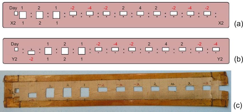
P. L. Woodworth: Tide prediction machines at the Liverpool Tidal Institute
www.hist-geo-space-sci.net/11/15/2020/
Table 1. (a) Inventory of tide prediction machines. (b) Inventory of portable tide prediction machines.
Sager no. Extra no. Kelvin Name Year Country Manufacturer No. of Country
prototype no. made made constituents now
(a)
TPM-KP1 Kelvin model made for the BAAS 1872 UK Messrs. White 8 UK
TPM-KP2 Kelvin Two-Component Machine 1873 UK L 2 UK
TPM-X1 Koenings’ Four-Component Machine Unknown France Unknown 4 Unknown
TPM-S1 Kelvin’s First TPM 1872–1873 UK L 10 UK
TPM-S2 India Office Machine 1879 UK L 24 India
TPM-S3 British TPM No. 3 1881 UK KW 16 France
TPM-S4 USCGS (US Coast and Geodetic Survey) No. 1 1882 USA Fauth & Co. 19 USA
TPM-X2a Australian TPM (Inglis No. 1) ∼ 1897 Australia A. Inglis 16 Unknown
TPM-X2b Australian TPM (Inglis No. 2) Unknown Australia A. Inglis 9 Unknown
TPM-S5 Roberts–Légé Machine 1906–1908 UK L 40 UK
TPM-S6 USCGS No. 2 1894–1910 USA US C&GS 37 USA
TPM-S7 British TPM No. 4 1909 UK KW 12 Brazil
TPM-S8 Japan Kelvin Machine No. 1 1914 UK KBB 15 Destroyed
TPM-S9 German TPM No. 1 1915–1916 Germany Toepfer & Sohn 20 Germany
TPM-S10 Argentina TPM No. 1 1918 UK KBB 16 Argentina
TPM-S11 Japan Kelvin Machine No. 2 1924 UK KBB 15 Japan
TPM-S12 Japan Kelvin Machine No. 3 1924 UK KBB 15 Japan
TPM-S13 Lisbon Machine 1924 UK KBB 16 Portugal
TPM-S14 Bidston Kelvin Machine 1924 UK KBB 29 France
TPM-S15 Brazil Kelvin Machine 1927 UK KBB 23 Brazil
TPM-S16 German TPM No. 2 1935–1939 Germany Aude und Reipert 62 Germany
TPM-S17 Russia Doodson–Légé Machine 1945 UK L 30 Destroyed
TPM-S18 Norway Kelvin Machine 1947 UK Chadburns 30 Norway
TPM-S19 Madrid Kelvin Machine 1948 UK KH 16 Spain
TPM-S20 Bidston Doodson–Légé Machine 1950 UK L 42 UK
TPM-S21 Manila Doodson–Légé Machine 1950 UK L 30 Philippines
TPM-S22 India Doodson–Légé Machine 1951 UK L 42 India
TPM-S23 Siam Doodson–Légé Machine 1951 UK L 30 Thailand
TPM-S24 Argentina Doodson–Légé Machine 1952 UK L 42 Argentina
Hist. Geo Space Sci., 11, 15–29, 2020
TPM-S25 German TPM No. 3 1952–1955 VEB Karl-Marx-Werk Germany 34 Germany
TPM-X3 Japan Doodson–Légé Machine 1956 UK L Japan
TPM-X4 Kobe Machine Unknown Japan Unknown Unknown
TPM-X5 Indonesia Doodson–Légé Machine ∼ 1963 UK L 30 Destroyed?
TPM-X6 Burma Doodson–Légé Machine ∼ 1964 UK L 42 Myanmar
(b)
Portable no. Name Year Country Manufacturer No. of constituents Number
made made made
PTPM-1 German Navy PTPM ∼ 1940 Germany Aude und Reipert 10 About 20
PTPM-2 British Copies ∼ 1947 UK Marine Instruments Ltd. 10 Unknown
PTPM-3 Doodson–Légé PTPM ∼ 1956 UK L 12 At least 12
Manufacturers: L – Alexander Légé & Co.; KW – Kelvin and White, Glasgow; KBB – Kelvin, Bottomley and Baird, Glasgow; KH – Kelvin and Hughes, Glasgow.
18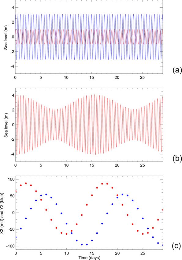
P. L. Woodworth: Tide prediction machines at the Liverpool Tidal Institute                                                               19

Figure 3. Photographs of the three Bidston TPMs: (a) the Bidston Kelvin Machine as normally seen in its casing and (b) an earlier photograph
showing more clearly the machine components, including the wheels for each tidal constituent and, on its right-hand side, the chart plotter.
(Photos: National Oceanography Centre and SHOM.) (c) The Roberts–Légé Machine at the Franco–British Exhibition of 1908, (d) being
refurbished in 2015 and (e) on display at NOC in Liverpool in 2019. (Photos: National Oceanography Centre, Philip Woodworth and Helen
Rawsthorne.) And (f) the Bidston Doodson–Légé Machine after being refurbished in 2015 with (g) a close-up of the pulley wheels for the
M10, Mm, M8 and MSf constituents between which a nickel band can be seen passing over or under each pulley. Each amplitude block
contains a Vernier screw with which to set the constituent’s amplitude, while its phase is defined using the wheel behind. The brass knobs
are the clutch controls for each constituent. (Photos: Philip Woodworth.)

   The most obvious product of the TPM was the ink trace on             stage, the individual sinusoidal motions would be arranged
a paper chart, similar to that produced by a traditional float          not as cosines summing to htotal but as a sum of the individ-
and stilling well tide gauge equipped with a chart recorder.            ual rates of change of height.
The fluctuations in the tide-like trace on the chart were pro-                               N
portional to those in the real ocean with a constant of propor-
                                                                                             X
                                                                        ∂htotal /∂t = −1.0         hi ωi sin (ωi t − gi )               (2)
tionality set by the machine design.                                                         i=1
   However, in practice, what most people needed to know
was simply the heights and times of high and low waters, not               The machine operator would run the machine, set up for
a continuous time series given by a trace on a chart. The pro-          the year required for prediction, and note the times t when
cedure for providing this information using most machines               ∂htotal /∂t happened to be zero, usually four times per day.
was to set up the machine for use in two stages. In a first             The machine would then be set up so as to provide Eq. (1),
                                                                        and the operator would make a note of the heights corre-

www.hist-geo-space-sci.net/11/15/2020/                                                         Hist. Geo Space Sci., 11, 15–29, 2020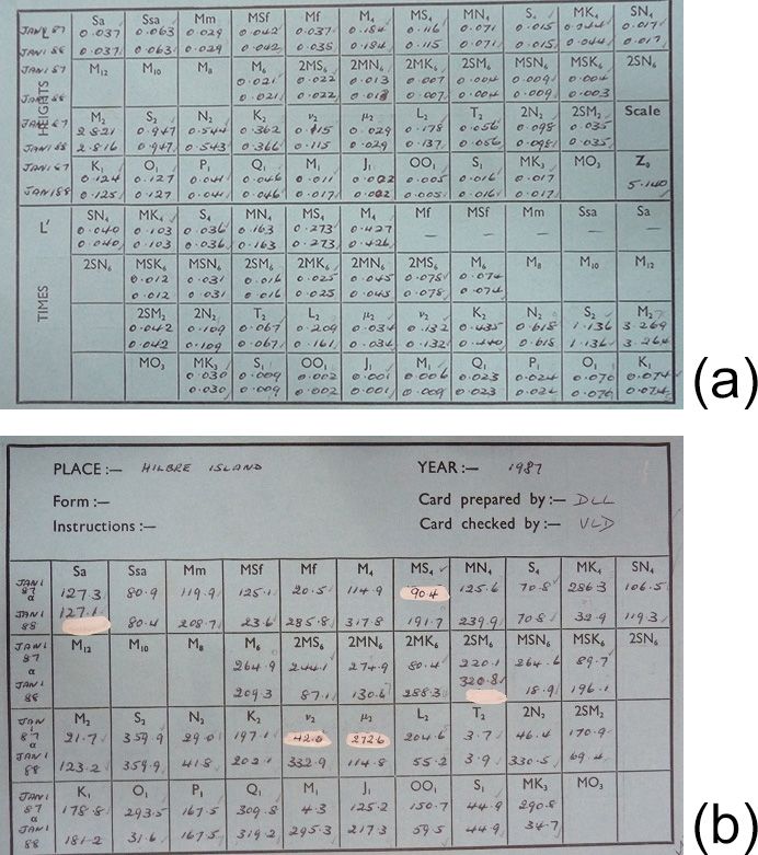
20                                                       P. L. Woodworth: Tide prediction machines at the Liverpool Tidal Institute

sponding to each turning point time t. The operator would                Sager corresponded with Doodson and received help in the
then have all the information required for a tide table.                 compilation of his inventory.
   If funds allowed, then it was highly desirable to have a                 Table 1a contains a line for each TPM with a code num-
TPM that was double sided. In this case, the machine was                 ber such as TPM-S20, indicating that the machine was num-
two machines in one, with one side calculating the rates and             ber 20 in Table 2 of Sager (1955); TPM-KP1, indicating
the other side the heights (Eqs. 2 and 1 respectively). Instead          Kelvin’s first prototype; TPM-X1, indicating a machine that
of a paper chart, the instantaneous rates and heights at time            was not in Sager’s 1955 inventory; or PTPM-1, indicating the
t would be displayed on a panel on the front of the machine,             first portable tide prediction machine (PTPM). Sager did not
and the operator would simply have to note the heights and               include the prototype machines of Kelvin, presumably be-
times when rates were zero. As a result, there was a major im-           cause they were never used for operational tidal predictions.
provement in the overall efficiency of the work. The Bidston             In addition, there were a couple of omissions such as the two
Doodson–Légé Machine (TPM-S20) provides a good exam-                     Australian TPMs. His book was published in 1955, just as the
ple of this. When first constructed in 1950 it was a single-             production of the machines was coming to an end, but there
sided machine, until funds could be made available in 1956               were still at least three to come along, including the Japan,
to enable its conversion to a double-sided machine.3                     Indonesia and Burma (Myanmar) Doodson–Légé machines
   Figure 2 provides only a schematic description of a TPM.              denoted TPM-X3, X5 and X6 in Table 1a. In addition, he did
However, while the principles of construction of each ma-                not include the smaller portable TPMs that were developed
chine were much the same, their mechanical design differed               for military and hydrographic surveying purposes; those that
in detail. Therefore, if one looks into aspects of a particular          I know about are listed in Table 1b. As far as I know, they
machine now, it may be difficult to obtain a complete under-             were not a great success and never became as well-known as
standing without access to copious original documentation.               the larger machines.
                                                                            Table 1a includes each machine name and the year and
                                                                         country of its manufacture, together with the manufacturer’s
4    TPM inventory
                                                                         name. It also shows the number of constituents in its design
An updated “inventory” has been made recently of all the                 and the country where the machine is now located. Wood-
TPMs that were made by various groups around the world                   worth (2016) contains more details for some of them. For ex-
(Woodworth, 2016). Tables 1 and 2 are based on the corre-                ample, when a machine was refurbished, extra constituents
sponding tables in that report.                                          were sometimes added, such as the conversion from 20 to
   A first inventory was made by the International Hydro-                24 constituents for TPM-S2 during its refurbishment in 1891.
graphic Bureau in 1926 (IHB, 1926).4 This was a collec-                     It can be seen from Table 1a that most of the machines
tion of sets of information provided by the machine own-                 were associated with a particular manufacturer and so with
ers at the time. However, Arthur Doodson remarked that                   a particular architecture. As mentioned above, the invention
the report could have been done better (Doodson, 1926). A                of the TPM is usually credited to Kelvin and all TPMs are
second inventory was made in 1955 by the oceanographer                   sometimes called Kelvin machines. However, “Kelvin-type”
Günther Sager from Germany. Chapter 3 of his “Gezeiten-                  machines can also refer simply to the set of machines made
voraussagen und Gezeitenrechenmaschinen” is entitled “Zur                in Glasgow (also in London and Basingstoke) by companies
geschichtlichen Entwicklung der Gezeitenrechenmaschinen”                 that were associated with Kelvin or, after his death, contin-
or “The Historical Development of Tide Calculators”. It con-             ued to carry his name (Table 1a). These “Lord Kelvin Tide
tains a list of the 25 TPMs that he knew about and gives some            Predictors” are referred to further in Table 2. The Norway
technical details of each one. In this case, it is known that            Kelvin Machine (TPM-S18) was also a Kelvin type, although
                                                                         it was made by Chadburns of Liverpool and not by one of the
    3 The two sides of the machine were known at the LTI as the          Kelvin companies.
times and heights sides, rather than the rates and heights sides. The       In addition, there were a number of machines, following
LTI names referred to the intended application, which was to com-        the Roberts–Légé Machine of 1906 (TPM-S5), that could
pute the times and heights of high and low waters. Two dials can         be described as “Légé type” (or “Roberts–Légé type” or
be seen on the left-hand side of the front of the machine beneath        “Doodson–Légé type”). This applies to the later machines,
the paper chart cylinder and above a panel showing the date and          designed or supervised by Edward Roberts or Arthur Doo-
time (Fig. 3f). The left-hand dial displays the rates (or “gradients”
                                                                         dson. These were manufactured by the London scientific
as Doodson, 1951, referred to them), for use either when the orig-
                                                                         equipment company of Légé & Co. The Kelvin and Légé
inal single-sided machine was set up to provide Eq. (2) or now us-
ing the times (back) side of the present double-sided machine. The       type architectures were quite different, the companies retain-
right-hand dial displays the heights, for use either when the original   ing those distinctive architectures for many years. For exam-
machine was set up for Eq. (1) or now using the heights (front) side     ple, the Roberts–Légé Machine (TPM-S5) and the Doodson–
of the present machine.                                                  Légé Machine (TPM-S20), made a half-century apart by the
    4 An even earlier list of the small number of machines in exis-      Légé company, have a similar number of constituents and
tence at the time was given in USCGS (1915).                             look very similar. However, the Légé-type machines tended

Hist. Geo Space Sci., 11, 15–29, 2020                                                      www.hist-geo-space-sci.net/11/15/2020/
P. L. Woodworth: Tide prediction machines at the Liverpool Tidal Institute                                                              21

Table 2. Lord Kelvin Tide Predictors. The machines made by the Kelvin companies carried plaques that gave the machine a “Lord Kelvin
Tide Predictor” number. This table provides a list of these machines.

     Sager No.    Lord Kelvin Tide     Name                             Comments
                     Predictor No.
              3                  1?    British TPM No. 3                Now in France. Plaque does not give a number.
              7                  2?    British TPM No. 4                Now in Brazil. Plaque does not give a number.
              8                    3   Japan Kelvin Machine No. 1       Machine destroyed in earthquake.
            10                     4   Argentina TPM No. 1              Plaque missing from the machine but almost certainly “No. 4”.
            11                     7   Japan Kelvin Machine No. 2       Photo of plaque available.
            12                     8   Japan Kelvin Machine No. 3       Photo of plaque available.
            13                     5   Lisbon Machine                   Photo of plaque available.
            14                     6   Bidston Kelvin Machine           Now in France. Photo of plaque available.
            15                     9   Brazil Kelvin Machine            Photo of plaque available.
            18                   10    Norway Kelvin Machine            We assume this counted as “Lord Kelvin Tide Predictor No. 10”
                                                                        so that the Madrid Kelvin Machine was later considered by KH
                                                                        as “No. 11”. The Norway Kelvin Machine was made by Chad-
                                                                        burns and not KBB/KH and does not have a plaque. But there
                                                                        is no other candidate for “No. 10”.
            19                   11    Madrid Kelvin Machine            Photo of plaque available.

to be more solid in construction, with moving parts for the              Such travel was essential, as Légé had not made a similar
harmonic motion made in steel instead of brass, and there-               machine for almost half a century since TPM-S5. It is unfor-
fore they were more expensive.                                           tunate that the Russia Doodson–Légé Machine is one of the
   Although there were important TPMs constructed in Ger-                few machines not to survive, although in fact it is the only
many and the USA (USCGS, 1915; Hicks, 1967; Cartwright,                  one for which there is a historical record on film (Tide and
1999; NOAA, 2019), the majority were designed and man-                   Time, 2019). The so-called Siam (Thailand) Doodson–Légé
ufactured in the UK. Of the 33 machines in Table 1a, 25 of               Machine (TPM-S23) was made to a particularly high stan-
them were made in either London, Glasgow or Liverpool. In                dard and was displayed in the “Dome of Discovery” at the
addition, the UK was the only country to export TPMs to                  Festival of Britain in 1951.
other countries. The construction of the majority of the ma-                After Doodson’s retirement in 1960, the liaison with Légé
chines made after 1920 was supervised, one way or other,                 was taken over by Jack Rossiter, the new director at Bid-
by Arthur Doodson. He oversaw the construction by Légé of                ston. This included the manufacture of machines for Indone-
machines for Russia, Bidston, Philippines, India, Thailand,              sia and Burma (TPM-X5 and X6). Scoffield (2006) mentions
Argentina and Japan (TPM-S17, S20–S24 and X3) and pro-                   that Légé & Co. may have also been trying to sell another
vided advice to prospective purchasers of other machines,                machine to Mexico in early 1965 and was unhappy when
such as that made for Norway by Chadburns (TPM-S18).5                    Rossiter suggested selling them the Roberts–Légé Machine
Those that he inspected were awarded a “Certificate of Ef-               (TPM-S5) instead. However, neither proposal came to any-
ficiency”. The Russia Doodson–Légé Machine (TPM-S17)                     thing, and subsequently Bidston terminated its relationship
required a particular effort, involving many trips by Doodson            with Légé on the advice of the solicitors of Liverpool Uni-
from Bidston to the Légé factory in London during wartime.               versity owing to the company’s financial difficulties.
                                                                            TPMs provide just one example of how analogue machines
   5 Doodson had also evidently been in contact with the Hydro-          undertook routine mathematical tasks in a wide range of sci-
graphic Department of the Chinese navy concerning the acquisition        entific research before digital computers became available,
of a machine. A letter from the navy to Doodson in December 1947         and Tables 1 and 2 show that they were employed by tidal
stated that they had ordered one from Marine Instruments Ltd. (i.e.      agencies in many countries. Rawsthorne (2019) has con-
KBB). However, there is no evidence that such a machine was de-          ducted a “prosopographical study” of this entire inventory
livered. Much earlier, Doodson had heard from KBB in 1931 that           of TPMs, in a study of how ideas and technology are spread
they had been approached about a machine for China, but nothing          around the world. Analogue machines continue to have an
seems to have come of that either.

www.hist-geo-space-sci.net/11/15/2020/                                                         Hist. Geo Space Sci., 11, 15–29, 2020
22 P. L. Woodworth: Tide prediction machines at the Liverpool Tidal Institute
important role in many modern research fields (MacLennan, These two TPMs equipped Doodson with experience that
2018). would prove invaluable when considering the design of later
machines. They would also provide him with the means to
5 The three TPMs at the LTI enable the LTI to become one of the main producers of tide
tables worldwide. The two machines were to play particu-
Most of the funding for the establishment of the LTI in 1919 larly important roles in World War II, in providing tidal pre-
had come from Sir Alfred Booth and his brother Charles dictions for D-Day and for other military operations in Eu-
Booth of the Booth Shipping Line in order to “prosecute con- rope and the Pacific. Those for D-Day were unusual in that
tinuously scientific research into all aspects of knowledge of they were made for an unknown location (now of course
the tides” (Doodson, 1924; Carlsson-Hyslop, 2020). known to be Normandy), using only the crudest of harmonic
In 1925, Charles Booth also provided most of the constants provided by Commander Farquharson at the Tidal
GBP 1500 required for the purchase of a 25- to 28- Branch of the Admiralty (Parker, 2011). However, they were
component TPM for the exclusive use of Doodson at the LTI. not secret for long. In July 1944, Doodson gave a lengthy in-
The BAAS contributed GBP 300. In the event, this became terview to the Liverpool Daily Post, stressing the importance
a 26-component machine, later extended to 29 components. of the TPMs to the D-Day predictions (LDP, 1944).
This Bidston Kelvin Machine (TPM-S14) was made by the In 1947, Doodson asked Légé to estimate the price of
firm of Kelvin, Bottomley and Baird of Glasgow with Doo- a machine with at least 35 components. Légé produced an
dson taking a great interest in its construction and suggest- initial design which Doodson started working on in detail.
ing modifications. It stood about 7 feet (2.1 m) high, 6 feet This became the 42-component machine delivered finally by
(2 m) long and 2 feet (0.6 m) wide and was encased by sliding Légé in December 1950 at a cost of GBP 5049 (Woodworth,
doors (Doodson, 1925, 1926, 1927). Figure 3a and b show 2016).6 This Bidston Doodson–Légé Machine (TPM-S20),
photographs of the machine. referred to by Bidston staff as the “D–L machine”, was the
Then in 1929, following the death of H. W. T. Roberts (the third machine to be used operationally at the LTI and one
son of Edward Roberts), Doodson acquired the Légé-made of a number of similar machines made by Légé & Co. un-
machine that Edward Roberts had designed in 1906 and der Doodson’s supervision and exported to several countries.
which had won a Grand Prix at the Franco–British Exhibition Doodson (1951) describes it in some detail. It was a single-
of 1908. Roberts had subsequently used it as part of his own sided TPM, being converted to a double-sided machine in
tidal prediction business (Messrs. Edward Roberts & Sons of 1956. It has an aluminium frame, unlike the steel frame of
Broadstairs), with the work of that business, including pre- TPM-S5. The machine is approximately 7 feet (2.1 m) high,
dictions for the Hydrographic Office, also passing to the LTI 9.5 feet (3 m) long and 3.5 feet (1.1 m) wide and weighs 1.4 t
in 1929. Doodson paid the Roberts family GBP 753 15s 0d. (not including the support base frame). Complete engineer-
This Roberts–Légé Machine (TPM-S5) simulated 33 con- ing drawings and documentation survive which have enabled
stituents, several more than the Bidston Kelvin Machine. its recent restoration.7 Figure 3f and g provides photographs
By 1929 it was in need of an overhaul and refurbishment. of the machine.
Shortly thereafter, the number of constituents was increased The purchase of the Doodson–Légé Machine had been
to 40 by Chadburns of Liverpool, with its original design made contingent on the sale of the Bidston Kelvin Machine
having allowed for such a future expansion. Its dimensions to the Service Hydrographique et Océanographique de la Ma-
are approximately 7 feet (2.1 m) high, 6 feet (2 m) long and rine (SHOM) in France. It was acquired by them in 1950
2.5 feet (0.8 m) wide (somewhat wider with its casing). It re- and was operated first in Paris and then in Brest for predict-
mained in use at Bidston until 1960 (Scoffield, 2006). This ing the tides of overseas ports (SHOM, 2019). It remained
TPM was sometimes known as the “Universal Tide Predic- in operational use at SHOM until 1966 (Rawsthorne, 2019).
tor of 1906” and also as the “Roberts Tide Predicting Ma- Nowadays, the Roberts–Légé and Doodson–Légé machines
chine”, a name which had previously been attached to the In- are both on display at the National Oceanography Centre in
dia Office Machine (TPM-S2) which had also been designed Liverpool (Tide and Time, 2019), the only place in the world
by Roberts. Doodson and Bidston staff referred to it as the where two TPMs can be seen alongside each other. Mean-
“Légé machine”. Photographs of this machine are shown in while, the Bidston Kelvin Machine may still be found at
Fig. 3c–e. SHOM in Brest. All three machines are in working or near-
Doodson wrote in an internal note that there was no dif- working order.
ference in performance between the Bidston Kelvin and
Roberts–Légé machines. He stated that for both “the total er-
ror of production of a tide does not differ by more than 0.05 ft 6 Schoffield (2006) mentions that the initial estimate by Légé
(1.5 cm) and 1 min of time from calculations using the same was GBP 4150 for a single-sided machine that could be upgraded
harmonic constants, even for the largest ranges of tide”. as funding permitted.
7 There were some 5000 gear ratios involved in the design of the
Bidston Doodson–Légé Machine.
Hist. Geo Space Sci., 11, 15–29, 2020 www.hist-geo-space-sci.net/11/15/2020/P. L. Woodworth: Tide prediction machines at the Liverpool Tidal Institute 23
6 The required harmonic constants
Equation (1) shows that if one knows the amplitudes and
phases of each constituent at a point on the coast (known
collectively as the “harmonic constants” for that location),
then it is possible to compute the total tide htotal at that po-
sition for any time t, either by considerable arithmetic effort
or with the use of a TPM. However, how does one know the
harmonic constants in the first place?
Any calculation of the harmonic constants has to be based
on measurements made at the location by a tide gauge, pro-
viding a record of the sea level at every hour (for exam-
ple) for an extended period such as a month or year. At
one time, there were hopes that machines could perform a
harmonic analysis of each record, machines having been in- Figure 4. A group photograph of the team of computers at Bid-
vented during the 19th century to undertake many mathemat- ston Observatory in 1953. (Photo: Valerie Gane.) They are gathered
ical tasks (De Mol and Durand-Richard, 2016). Kelvin ap- around the original Liverpool One O’Clock Gun which, when lo-
cated in Birkenhead Docks, was fired by means of transmission of
plied the Disk-Globe-and-Cylinder Integrator developed by
an electrical signal from the Observatory.
his brother, James Thomson, to the evaluation of the inte-
grals needed for harmonic analysis and thereby to the deter-
mination of harmonic constants from an input time series of machines for mechanical harmonic analysis has continued to
tidal measurements. Kelvin called this “substituting brass for attract interest in science and engineering through the years
brain” (Thomson, 1881). (e.g. Webb and Bacon, 1962, and for a review see Durand-
A small number of such machines were made eventually. Richard, 2016b, Sect. 8.2.3).
Kelvin first constructed a model of a five-component ma- The harmonic analyser was a classic example of Kelvin’s
chine capable of analysing a time series from which one ingenuity. However, the machine had no lasting importance
could determine the cosine and sine components of two har- within tidal science, and, in the context of the present pa-
monic constituents together with a mean value. This ma- per, it was not relevant to the work of the LTI. Instead, the
chine is now on display at the Hunterian Museum of Glas- harmonic constants had to be determined by laborious arith-
gow University. A similar machine made by R. W. Munro metical methods by teams of (predominantly female at the
and Company was employed by the Meteorological Office LTI) assistants called “computers” (Fig. 4). In the following,
for the determination of daily variations in meteorological I outline the method developed at the LTI by Arthur Doodson
parameters (Thomson, 1878); this is now on display at the and put into practice by his team of computers. 9
Science Museum. However, for tides one needed a machine Before doing that, it is useful to recall that the two largest
capable of handling more harmonic terms. By 1879, an 11- tidal constituents in many parts of the world are M2 (the main
component machine had been made, specifically for applica- semi-diurnal tide from the moon with a period of 12 h 25 min,
tion to tides (Thomson and Tait, 1879; Thomson, 1881). It half a lunar day) and S2 (the main semi-diurnal tide from
was not a great success. Thomson and Tait (1879) remarked the sun with a period of 12 h, half a solar day). Most other
that “The machine has been deposited in the South Kens- constituents also have periods around either 12 or 24 (semi-
ington Museum”. Parts of it are now preserved in the Sci- diurnal and diurnal tides), while some have shorter periods
ence Museum store; a photograph of it is contained in De (shallow-water tides), and a few have periods of up to a year
Mol and Durand-Richard (2016). 8 Proudman (1920) and or more (long-period tides). Ideally, all of the most impor-
Hughes (2005) mention several later attempts at mechanical tant of these constituents need to be represented in the mech-
tidal analysers, although they do not seem to have been suc- anism of a TPM, requiring prior knowledge of the harmonic
cessful either. Of course, by then the numerical methods of constants.
tidal analysis devised by Darwin (1893), and later developed For present purposes, I focus on the derivation of the
by Doodson (1928) discussed below, had removed the ne- semidiurnal constants and use Liverpool as an example. At
cessity for mechanical analysers. However, the use of similar this location, M2 and S2 have amplitudes of 3.13 and 1.01 m
respectively. Because a solar day lasts 24 h, the S2 tide will
8 The 11 components were designed to determine the five tidal repeat itself twice a day exactly at the same time every day
constituents M2, S2, K1, O1 and P1 (i.e. h cos(g) and h sin(g) for (shown in red in Fig. 5a). M2 has a larger amplitude and
each) plus the mean water level. Proudman (1920) states that the
five constituents included M4 instead of P1, although that is not 9 A good impression of the working relationships between Doo-
supported by Thomson (1881, 1882) or the surviving Science Mu- dson and his team of computers and other staff at Bidston Observa-
seum documentation. tory is given by Scoffield (2006).
www.hist-geo-space-sci.net/11/15/2020/ Hist. Geo Space Sci., 11, 15–29, 202024 P. L. Woodworth: Tide prediction machines at the Liverpool Tidal Institute
Figure 6. (a) A schematic version of an original cardboard stencil
for X2 with holes to show through those hours with data that had
to be multiplied either by positive or negative weights. (b) A cor-
responding stencil for Y2. (c) An original cardboard stencil for Y2
showing the positive (black) and negative (red) weights. There were
many pieces of cardboard like this for the different filters described
in Doodson (1928). (Schematic versions courtesy of Ian Vassie.)
plied by 2, being replaced by the nearest integer (i.e. ±2, ±1
and 0). In addition, setting t = 0 in the middle of the record
simplified the calculations, as cosines were required to be
multiplied only by cosines and sines only by sines. Further-
more, the method had some in-built redundancy, enabling a
check on the quality of the computations and on the possibil-
ity of there being unexpected constituents in the record. The
method is said to have revolutionised the analysis of tidal
Figure 5. (a) A schematic example of the variation of M2 (blue) observations in many countries (Proudman, 1968). Normally
and S2 (red) at Liverpool over a month, (b) M2 and S2 in combi- 1 year of tide gauge data was adequate, with observations of
nation and (c) the corresponding time series of daily values of X2 the water level every hour, i.e. 8640 values in a 360 d year.
(red) and Y2 (blue). (Doodson, 1954, described how shorter records may be anal-
ysed using similar methods.) His team of computers usually
worked with values of water level in units of one tenth of a
repeats twice a lunar day (a little later each solar day), as foot.
shown in blue. They combine by “beating together”, result- The method is described in detail in Doodson (1928)
ing in a total tide that is larger and smaller over a fortnight (see also Doodson and Warburg, 1941; Doodson, 1954).
(spring and neap variation, Fig. 5b). The separate contribu- The work was labour intensive, involving endless arithmetic.
tions of M2 and S2 to the total tide would not be readily However, Doodson claimed that an experienced computer
apparent with just 1 d of data, but the fact that they both ex- could analyse the tabulated hourly heights to determine about
ist becomes obvious when looking at this simple variation 40 constituents in 10 working days of 6 h each, with 1 d for
over a fortnight. However, the existence of other semidiurnal sundry checks by other computers. The analysis for 20 more
constituents complicates things. constituents would take another 6 h.
Doodson’s method of analysis of the hourly record made In this method it was not necessary to manipulate all 8640
use of ingenious arithmetical filters designed to magnify the hourly water levels at once. 10 A first step involved the use
importance within the record of each constituent in turn, and of a set of filters to convert the hourly information into daily
so, after a lot of work, to arrive at a set of estimates of their numbers, which have 24 times less the bulk of the original
amplitudes and phases. The multiplier coefficients of the var- record. For the semi-diurnal constituents, these filters were
ious filters in effect functioned as a form of least-squares called X2 and Y2 and were a set of simple integer arithmetic
fit similar to the way constituents are determined in modern weights applied to the hourly values for each day. Other inte-
harmonic analysis. However, Doodson refused to be bound
rigidly by the method of least squares, adopting it only as a
guide to his own method. Consequently, multiplications by
cosines and sines in the calculation of his coefficients were 10 Darwin (1893) had adopted a similar necessary approach of
deemed to be unnecessary, with the cosines and sines, multi- reducing the size of tidal data sets to manageable proportions.
Hist. Geo Space Sci., 11, 15–29, 2020 www.hist-geo-space-sci.net/11/15/2020/P. L. Woodworth: Tide prediction machines at the Liverpool Tidal Institute 25
ger filters were designed for diurnal variations and other tidal L2, T2, R2 and K2) fall into “groups” according to the pe-
components. 11 riods of their perturbation of X2 and Y2, with the group q
The computer listed on a page the hourly tide gauge val- perturbing X2 and Y2 by q complete periods per month. One
ues from hours 0 to 23 each day, with one line for each day, can determine the magnitude of these perturbations for each
and then used a cardboard cut-out called a stencil, with holes group with a filter defined by another set of integer multipli-
for those hourly values which were to be multiplied by a fil- ers, one set of multipliers for each group. This yields a set of
ter weight for each hole. The spacing of values written on values denoted as, for example, X2q which refers to X2 after
the page clearly had to be chosen so that the correct num- application of the multipliers for group q. This set X2q (and
bers would show through the appropriate holes in the stencil; similarly Y2q) consists of 12 numbers, one for each month
suitable paper was especially printed for this purpose. The in the year.
weight values themselves were written on the cardboard as Similarly, one will realise that each harmonic constituent
shown schematically for the X2 filter in Fig. 6a. within the group q will contribute to the set of 12 X2q values
The X2 filter for a particular day used data for hours 0–23 differently over a year. Consequently, by a suitable combina-
on that day and also hours 24–28 (i.e. hours 0–4 on the next tion of X2q values, a quantity called X2qr can be obtained,
day), spanning 29 h total. The integer weights were where r signifies the number of periods of variation of X2q
in the year. In general, a single X2qr (and Y2qr) corresponds
[1, 0, 2, 0, 1, 0, −2, 0, −4, 0, −2, 0, 2, 0, 4, 0, 2, 0, to a particular harmonic constituent.
− 2, 0, −4, 0, −2, 0, 1, 0, 2, 0, 1, 0, 0, 0]. The first task of the computer was to calculate X2 and
Y2 for each day, with the work done either by hand (which
The central value of the filter is shown underlined. The Y2 would take a considerable amount of time) or more usually
weights employed hours 3–23 on the required day and 24–31 later on with the use of a comptometer machine. She would
on the next day and had the values then write the values for each day in a table with 12 columns
(for 12 months of the year), with some columns having 29
[0, 0, 0, 1, 0, 2, 0, 1, 0, −2, 0, −4, 0, −2, 0, 2, 0, 4, 0, 2, 0, rows and some having 30 rows. X2 (or Y2) values for days
− 2, 0, −4, 0, −2, 0, 1, 0, 2, 0, 1]. from the start to the end of the year (i.e. about 360 values)
would be listed down column 1 first, then down column 2 etc.
In this case the central value (shown underlined) is 3 h until the year was completed in column 12. Doodson (1928)
different from that of X2. Therefore, the two filters sam- called this exercise the “daily processes”.
ple orthogonal components of the semi-diurnal variation. A The X2 (or Y2) values in each of the columns of the
schematic version of the Y2 stencil is shown in Fig. 6b and 12 months in this table were then multiplied by sets of integer
an original cardboard one in Fig. 6c. One can readily apply weights for each group q. These were called “daily multipli-
these filters to our example Liverpool data, and the daily time ers” (Table XV of Doodson, 1928), and this procedure was
series of X2 and Y2 for Liverpool then appear as in Fig. 5c. called the “monthly processes”. Then, the weighted X2 (or
It can be seen that Fig. 5c has much the same information Y2) values in the 12 months of the year (denoted X2q and
content as Fig. 5b (i.e. variation of the tide over a fortnight Y2q) were multiplied by further sets of integer weights for
given two harmonic constituents) but with 24 times fewer each month called “monthly multipliers” (Table XVI of Doo-
numbers. The constant parts (the offsets) of the red and blue dson, 1928) to provide X2qr (or Y2qr) values. These were
curves come from S2 because S2 is the same every day, while called the “annual processes”.
the cyclic parts, which vary over a fortnight, come from M2. As a consequence, these different sets of multipliers will
Consequently, the red and blue offsets are a consequence of have resulted in individual totalled quantities (X2qr or Y2qr)
the amplitude and phase of S2, while the cyclic parts depend which, after a further “correction” stage for leakage into the
on the amplitude and phase of M2.12 X2qr and Y2qr from a small number of other constituents,
However, it can be appreciated that this simple situation will have magnified the importance of particular constituents
becomes more complicated when additional constituents are within the record and so ultimately have provided an esti-
taken into account. For example, one can expect that S2, as mate of the constituent’s amplitude and phase. For some con-
it manifests itself in Fig. 5c for a particular month, will ap- stituents such as S2, estimates of amplitude and phase were
pear different in the next month if there is also significant K2 given from the use of only certain multipliers (i.e. an indi-
present in the record, and those differences will vary over half vidual 2qr), but for others, such as K2, they were provided
a year. In practice, M2 and S2 and all of the remaining semid- through the use of more than one 2qr, requiring combination
iurnal constituents (such as 2N2, Mu2, N2, Nu2, Lambda2, in an additional stage.
11 The way that the X2 filter was selected is described in Sect. 5 Finally, because the analysis set t = 0 in the middle of the
of Doodson (1928). He remarked that “it is unnecessary to illustrate 1-year record, there was a need to adjust the derived ampli-
the genesis of the remaining formulae”. tudes and phases for the appropriate astronomical arguments
12 The sums of the weights of X2 and Y2 are zero, so changes in and nodal factors at that time. These could be computed us-
mean sea level do not contribute to the offsets for S2. ing standard formulae.
www.hist-geo-space-sci.net/11/15/2020/ Hist. Geo Space Sci., 11, 15–29, 202026 P. L. Woodworth: Tide prediction machines at the Liverpool Tidal Institute
It can be seen that this was a complicated and labour in-
tensive procedure, but it was straightforward once it could
be explained clearly to a computer with basic mathematical
skills equipped with one of the mechanical or electronic cal-
culating machines available at that time. The method is de-
scribed in detail in Doodson (1928) with a worked example
for a year of data from Vancouver 13 .
Doodson (1928) explained that his was not the first such
method. There were many papers published in the 19th cen-
tury which list amplitudes and phases for harmonic con-
stituents computed in different ways (e.g. see Baird and Dar-
win, 1885). Most of these will have used the method devised
by Thomson, Roberts and Darwin and published in BAAS re-
ports between 1866 and 1885 (e.g. Darwin, 1884). This was
the method employed by Roberts and the Survey of India to
determine amplitudes and phases for use with their TPMs.14
There was also Darwin’s later method (Darwin, 1893), of
which Doodson (1928) claimed his to be a further develop-
ment. There was a popular method invented in Germany by
Börgen (1894) which was studied for use in several coun-
tries (e.g. Adams, 1910). The US Coast and Geodetic Survey
also had its own method based on the intensive use of many
filters (USCGS, 1894). Doodson (1928) provides a short dis-
cussion of the relative merits of each method. They were said Figure 7. (a, b) The two sides of a relatively recent “running card”
to differ in the amount of labour involved (the BAAS method for use with the Bidston Doodson–Légé Machine, in this case for
was said to require the most labour; Börgen’s method re- producing predictions for Hilbre Island in 1987 and 1988. (Card
quired the least until Doodson’s became available); in how courtesy of Valerie Gane.)
well they could eliminate the overlap of information from
different constituents in the derivation of the amplitudes and
phases; and in the completeness of the analysis. However, so by similar filtering to that described above. All the ampli-
far as I know, there was never a detailed, quantitative com- tudes and phases were written on a special “running card”
parison between methods. 15 for the port in question and for the year requiring predic-
tion by the machine. These values were derived from “con-
stants cards”, which contained a list of amplitudes and phase
7 Setting up the TPM
lags for the particular port and from values of V , f and u
Doodson then had all the amplitudes and phases that he for the year in question, as explained below. Each “running”
needed to set up his TPM, including those of the semidiur- (or “setting-up”) card was colour coded according to the par-
nal, diurnal, shallow-water and long-period tides calculated ticular year. Figure 7a and b shows the front and reverse of
a relatively recent example of a card that was used for op-
13 However, this is not a complete worked example, and there are eration of the Bidston Doodson–Légé Machine (TPM-S20).
some errors e.g. p. 258 and Table XXX of Doodson (1928) refer to Those used earlier for the Doodson–Légé Machine and the
a datum value of 500 for X2, Y2 which should be 600. two other Bidston machines will have been similar.16
14 The India Office Machine was used to make the tidal predic- The top part of one side of the card (Fig. 7a) shows val-
tions for India and elsewhere, although it was located first in Eng- ues for f times amplitude for each constituent, in the order
land for over 40 years, first at Lambeth and then at the National that the constituents appear on the front of the machine, for
Physical Laboratory in Teddington, until it was moved in 1921 to Hilbre Island (near Liverpool) for 1 January 1987 and 1988.
the headquarters of the Survey of India in Dehra Dun. The values are in metres, and the lunar ones such as M2 are
15 Tidal constants from many coastal locations produced by the
slightly different for the 2 years because their nodal factors
LTI and other national tidal agencies would eventually form the ba-
f vary from year to year (Pugh and Woodworth, 2014). In
sis of the International Hydrographic Organization tidal databank
(Qi, 2012). In turn, the databank would aid the development of re- fact, January 1988 was close to a nodal minimum for M2.
gional and global tidal charts and tide models. The construction of
tidal charts had been an important research topic since the middle of 16 Most running cards were colour-coded and contained informa-
the 19th century (e.g. Whewell, 1833) and was one in which Dood- tion for only 1 year. However, the values for the 2 years shown in
son himself had been engaged in the early years of the LTI (Proud- this particular example are useful in demonstrating the nodal depen-
man and Doodson, 1924; Cartwright, 1999). dence of the lunar constituents.
Hist. Geo Space Sci., 11, 15–29, 2020 www.hist-geo-space-sci.net/11/15/2020/You can also read