Time in Office and the Changing Gender Gap in Dishonesty: Evidence from Local Politics in India - Graduate Institute
←
→
Page content transcription
If your browser does not render page correctly, please read the page content below
Time in Office and the Changing Gender Gap in
   Dishonesty: Evidence from Local Politics in India∗
                       Ananish Chaudhuri† Vegard Iversen‡
                      Francesca R. Jensenius§ Pushkar Maitra¶
                                           May 2021

                                             Abstract
       Increasing the share of women in politics is often touted as a means of reducing
       corruption. In this study, we focus on dishonesty among elected male and female
       representatives, and how this changes with time in office. We combine survey data
       on attitudes towards corruption with data from incentivized experiments. Our
       sample consists of 400 inexperienced and experienced local politicians in West
       Bengal, India. While we find little evidence of a gender gap in the attitudes of in-
       experienced politicians, experienced female politicians exhibit a stronger distaste
       for corruption. However, this apparent hardening in attitudes among female politi-
       cians also coincides with more dishonest behavior in our experiments. Exploring
       mechanisms that can explain this difference, we find it to be strongly associated
       with lower risk aversion and weaker political networks. Our study indicates that
       gender gaps in politics should be theorized as dynamic and changing, rather than
       static.

   ∗
     We gratefully acknowledge funding from the University of Auckland, Monash University, and the
Norwegian Research Council (project number 250753). IRB clearance obtained from University of
Auckland (Approval number 019938). We thank the field staff at Outline India for conducting the
surveys and experiments that we report from. We thank the field staff at Outline India for conducting
the surveys and experiments reported. The paper has benefited greatly from comments at several
seminars and conferences, although the authors remain responsible for any errors.
   †
     Professor, Department of Economics, University of Auckland, New Zealand.                 E-mail:
a.chaudhuri@auckland.ac.nz
   ‡
     Professor of Development Economics and Head of Livelihoods and Institutions Department, Uni-
versity of Greenwich, United Kingdom. E-mail: vegard.iversen@gre.ac.uk.
   §
     Corresponding Author. Professor, Department of Political Science, University of Oslo, Norway.
E-mail: f.r.jensenius@stv.uio.no
   ¶
     Professor,    Department of Economics,       Monash University,        Australia.        E-mail:
pushkar.maitra@monash.edu.au
1 Introduction
The under-representation of women in political life has galvanized efforts to ensure that
more women stand for and win elections. Arguments in favor of increased political
presence of women include ideas of fairness and social justice; that women’s experiences
and perspectives are distinct, valuable and deserve to be heard; and that women, as well
as other under-represented groups, can serve as role models (Phillips 1995; Wangnerud
2009; Campbell, Childs and Lovenduski 2010).
Increased female representation has been found to shift policy agendas and develop-
ment outcomes (see Chattopadhyay and Duflo 2004; Betz, Fortunato and O’Brien 2021;
Clayton and Zetterberg 2018); improve women’s access to the state (Iyer et al. 2012);
and raise the quality of politicians (Besley et al. 2017). It is also argued that increasing
the share of women in politics may improve governance and reduce corruption, with
research indicating that women are more trustworthy (Dollar, Fisman and Gatti 2001;
Schneider and Bos 2014; Barnes and Beaulieu 2019), more averse to risk-taking (Croson
and Gneezy 2009; Eckel and Grossman 2002; Roszkowski and Grable 2005; Fletschner,
Anderson and Cullen 2010), and lack the political networks required to engage in malfea-
sance (Heath, Schwindt-Bayer and Taylor-Robinson 2005; Goetz 2007; Bjarnegård 2013;
O’Brien 2015).
Cross-country and cross-regional evidence indicates that having a higher share of
women in parliament or in the bureaucracy is associated with lower corruption (Dollar,
Fisman and Gatti 2001; Grimes and Wängnerud 2010). Studies using individual-level
data have also found women to be more honest and less tolerant of corruption (Friesen
and Gangadharan 2012). In India, Duflo and Topalova (2004) report that villagers are
less likely to pay bribes if the village headship is reserved for women. Baskaran et al.
(2018) find that the annual rate of asset accumulation among female members of state
legislative assemblies is 10 percentage points lower than for men. Brollo and Troiano
1(2016) report that female mayors in Brazil are less likely to be involved in administrative
irregularities.
Other studies, however, find no gender disparity in the propensity to be corrupt or
dishonest (Sung 2003; Vijayalakshmi 2008; Debski et al. 2018). Some scholars have tried
to reconcile these seemingly contradictory research findings by arguing that the gender
gap in dishonesty is more pronounced in democracies with high electoral accountability
(Alatas et al. 2009; Esarey and Schwindt-Bayer 2018). Others hold that the observed
association between gender and corruption is spurious, as liberal democracies are likely
to have less corruption and greater gender equality (Sung 2003).
Less studied is how time in office affects politicians’ attitudes and behaviors.1 In this
paper, we theorize the nature of the gender gap in dishonesty as changing, or dynamic.
As earlier studies have found women to be more pro-social, more risk-averse, and to
have weaker political networks than men, women could be expected to be less corrupt
than men when they enter office. However, these characteristics may change with the
experience of holding political office. Although such change may occur for both men
and women, we would expect a greater change for women, as the political culture they
enter into is likely to be further from their previous experiences than is the case for men,
especially in gender-segregated societies.
Empirically studying corrupt behavior in politicians is challenging, as self-reported
responses are prone to self-reporting and social-desirability biases, and elected politi-
cians are not a readily accessible pool of subjects for experimental work. Therefore,
studies attempting to capture the intentions and behavior of real-world politicians often
employ proxies and indirect measures, such as the quality of program delivery in their
constituency or aggregate regional/country-level indicators of corruption. By contrast,
1
An exception is Afridi, Iversen and Sharan (2017), who find more administrative lapses and program
leakages in villages with women village council heads compared to councils with men in power, but only
during their first year in office.
2experimental studies of individual-level behavior typically rely on citizen participants—
often university students from industrialized countries. That limits the scope for extrap-
olating findings to elected politicians, as the observable and unobservable characteristics
and attitudes of politicians are likely to differ greatly from those of the general citizenry
(Dal Bó et al. 2017; Chaudhuri et al. 2021).
For this study, we collected a comprehensive survey and experimental dataset cover-
ing a sample of 400 local male and female politicians in West Bengal, India. To measure
propensity towards dishonest behavior, we used questions and vignettes to reveal atti-
tudes towards corruption, as well as a die-tossing experiment in which participants were
asked to throw an unbiased die 30 times in private, with payment received based on
the number of sixes they report (see Fischbacher and Föllmi-Heusi 2013). There was
no monitoring of the actual number of sixes reported, so we cannot know for certain
whether an individual cheated. However, we can use the deviation of the actual number
of sixes reported from simulated or theoretical distributions of the number of sixes in 30
throws of an unbiased die to obtain a group-wise measure of dishonesty.2
We report two main findings. First, whereas there is little overall difference in atti-
tudes towards corruption among male and female politicians in the self-reported survey
data, experienced politicians in our sample, particularly women, express markedly lower
tolerance of corruption. The experimental data, however, reveal a gender gap in be-
havior. Among inexperienced politicians, women report fewer sixes than men in the
die-tossing task; and among experienced politicians, women report significantly more
sixes than men. However, we found no observable difference between experienced and
2
While we do not equate corruption with dishonest behavior, we expect those who behave dishon-
estly in our incentivized die-tossing game to be more prone to corruption behavior when given the
opportunity. A large and credible body of evidence now supports the assumption that behavior in the
game is a reliable indicator of corruption (see, e.g., Cohn, Marechal and Fehr 2014; Banerjee, Baul and
Rosenblat 2015; Hanna and Wang 2017; Kröll and Rustagi 2016; Dai, Galeotti and Villeval 2017).
3inexperienced male politicians. These findings indicate a pronounced time-in-office effect
on dishonest behavior among female, but not among male, politicians.3
Drawing on the theoretical discussion, we then test four possible mechanisms behind
the changing gender gap in dishonest behavior: differences in pro-sociality (altruism
and/or trustworthiness), risk aversion, access to political networks, and political as-
pirations. We use the behavior of participants in a dictator game and a trust game
to elicit pro-sociality, an investment game to measure risk aversion, use dynastic links
to estimate access to political networks, and examine responses to survey questions to
capture differences in political aspirations. We find no support for the hypothesis that
greater dishonesty is a result of female politicians becoming less pro-social or because
of differences in their political aspirations. However, we do find strong evidence for
women being more risk-averse than men when taking office, and for experienced female
politicians being significantly less risk-averse than their inexperienced counterparts. We
also find that these patterns are driven by the sample of politicians without dynastic
links—suggesting that the changes we observe are driven by women who enter politics
with weak political networks.
These findings make several contributions to the literature. To the best of our knowl-
edge, our study is the first to measure both self-reported attitudes and experimental
behavior on the topic of corruption in a large sample of elected politicians.4 Further, by
comparing inexperienced and experienced politicians, we present evidence on how behav-
ior may change with time in office, exposure to specific political environments and the
differentiated ways in which newly elected female and male representatives experience
these environments. Our findings that the behaviors of inexperienced and experienced
3
This discrepancy between attitudes and behavior echoes other work comparing survey and ex-
perimental data, and serves as a warning against reading too much into self-reported survey data on
sensitive topics (see Chaudhuri 2012).
4
However, survey experiments using actual legislators have become more common in political science
in recent years; see Naurin and Öhberg (2019).
4politicians differ and that considerable change emerges after as little as one term in office
provide valuable insights into the pace of behavioral change, and may also help reconcile
some of the seemingly contradictory conclusions about a gender gap in dishonesty found
by other studies.
2 A dynamic gender gap in dishonest behavior
Following the publication of Dollar et al.’s (2001) and Swamy et al.’s (2001) cross-country
analyses suggesting that having more women in parliament and other leadership posi-
tions reduces corruption, an emphasis on the instrumental value of women in positions
of power has spread widely. Reiterated in World Bank reports (e.g., WB 2002) and pol-
icy debates around the world, governments have acted swiftly on the idea that women
can help clean up politics. In 2003, for example, Mexico’s customs service announced
that its new anti-corruption force would be entirely female; and in Uganda, the vast
majority of positions as local government treasurers are assigned to women. Women are
increasingly being viewed as “political cleaners” (Goetz 2007).
Why is there a gender gap in corrupt or dishonest behavior among new entrants into
politics? A first explanation in the literature—which we will refer to as the pro-social
mechanism—is that women tend to be more altruistic than men. Many observational
and experimental studies support this argument. Evidence from dictator games suggests
that women are more generous (Eckel and Grossman 1998), while trust games show that
men are generally more trusting and women more trustworthy (see Rau 2012). Using
data from experiments conducted in Sweden, Dreber and Johannesson (2008) show that
women are less likely than men to lie in order to obtain a higher payoff; and D’Attoma,
Volintiru and Steinmo (2017, p. 2) find women to be more tax-compliant than men in
every country and under every condition studied. Similarly, a meta-analysis of sixty-
5three experimental studies finds that women appear to exhibit greater propensities to
tell the truth (Rosenbaum, Billinger and Stieglitz 2014). In a comprehensive review of
laboratory experimental evidence on gender differences in corruption, Chaudhuri (2012)
concludes that either women behave more honest than men, or there are no significant
gender differences.
A second explanation, also with ample empirical support, is that women tend to be
more risk-averse than men. We refer to this as the risk-aversion mechanism. Data from
the USA show that, as wealth increases, the proportion of wealth held as risky assets
is higher among men than among women (Jianakoplos and Bernasek 1998). Further,
in behavioral games with gambling options, men are more likely to choose risky bets
(Levin, Snyder and Chapman 1988). In their review of gender differences in economic
experiments, Croson and Gneezy (2009) conclude that there are robust differences in
male and female risk preferences. A gender gap in risk aversion has also been found in
studies of voters’ decisions, especially in high-stake political decisions (Verge, Guinjoan
and Rodon 2015). Applying these insights to a context of corruption, Schulze and Frank
(2003) show that whereas women are as willing as men to accept bribes in a no-risk
situation, they are less willing to do so in higher-risk situations.
The empirical expectation from both of these explanations is that, at the time of
entering office, female politicians are less likely than men to engage in corruption. How-
ever, neither of these explanations points to a static gender gap in attitudes or behavior.
To the extent that the differences result from socialization and experience rather than
from inherent differences between men and women, we should expect participation in
politics to re-socialize politicians.5 Newly elected politicians are likely—for better or
worse—to become socialized into the local version of the political game. Research from
Zambia, for instance, shows that holding office increases politicians’ adherence to a reci-
5
Essentialist versions of these arguments have encountered strong resistance from feminist scholars
(see, e.g., Phillips 1995; Goetz 2007).
6procity norm, indicating that with experience comes a greater likelihood of engaging in
corrupt behavior (Enemark et al. 2016).6 And the more the political environment differs
from the context politicians lived in before entering politics, the more change should we
expect to see in their behavior—not least as regards female politicians.
A third explanation for why women may engage less in corruption than men holds
that they have less opportunity, because of their weaker political networks (Heath,
Schwindt-Bayer and Taylor-Robinson 2005; Goetz 2007; Bjarnegård 2013; O’Brien 2015).
India is known to be a patronage democracy where much of the non-programmatic deliv-
ery of services, and probably also much of the corrupt behavior, occurs through networks
of brokers and activists (Chandra 2004; Bussell 2019). Indeed, female politicians have
been found to be less effective than men in navigating existing systems of patronage
(Bardhan, Mookherjee and Torrado 2005). People are also averse to working with fe-
male leaders, particularly in their first term in office (Gangadharan et al. 2016). This
network mechanism is a dynamic explanation that can help in explaining change over
time. Studies find that the people grow more accustomed to women leaders over time
(Beaman et al. 2009; Gangadharan et al. 2016) and that women rapidly build political
networks once they have a chance to do so (Goyal 2020).
If men and women face a similar political environment, we might expect their be-
havior to become more similar over time. However, some studies indicate that women
may become more prone to corrupt behavior as they gain political experience. First,
the literature on women’s experience of politics suggests that women face a more hostile
environment than men: they get less credit for the work they do, and experience nega-
tive attention, sexual harassment, and violent and other backlashes once in office (Krook
2016; Jensenius 2019; Mayaram 2002; Brulé 2020). This may harden their outlook on
6
This is consistent with studies of risk perception that find that those who are more familiar with
the risks they are exposed to are also less likely to perceive them as frightening (Cutter, Tiefenbacher
and Solecki 1992). Risk attitudes are influenced by social learning and environmental conditions and
can change rapidly—even within the span of weeks (Booth, Cardona-Sosa and Nolen 2014).
7political life. Second, we know that politicians with a shorter time horizon tend to be
more opportunistic while in office (Ferraz and Finan 2011). The changes in attitudes
and behavior during time in office that we observe may therefore be driven by women
becoming less interested in a future political career. We refer to this as the aspirations
mechanism.
3 Context and data
Our data are from West Bengal, a large state in Eastern India. India is a classic exam-
ple of a developing country where it is expected that politicians will engage in corrupt
behavior, with the media regularly reporting on scams and corruption scandals. Accord-
ing to Transparency International’s Corruption Perceptions Survey 2018, 56% of Indians
reported paying bribes for services in the previous year. Studies of the sworn affidavits
that politicians must submit before running for office show that many members of leg-
islative assemblies accumulate sizable wealth during their time in office (Fisman, Schulz
and Vig 2014). Bribe-paying may be increasing (Borooah 2016).
The 73rd Amendment to the Indian Constitution, ratified in April 1993, established
and codified a three-tiered system of local governance (the panchayat system), com-
prising councils at the village, block (or sub-district), and district levels. Although the
panchayat system had existed in many Indian states since the 1950s, it was not until
the mid-1990s that regular elections were held and village councils started playing more
than a limited role. West Bengal was an exception. When the Marxist CPI(M)-led Left
Front government came to power in West Bengal in 1977 on a platform of agrarian and
political reforms, revitalizing the panchayat system became a key priority. The first
panchayat election took place in 1978, with elections held every five years since then.
Thus, the decentralization mandated by the Amendment was already well established in
8West Bengal (see, Bhattacharya 2002; Ghatak and Ghatak 2002). A novel and radical
feature of the 1990s panchayat reforms was the mandated political reservations for mi-
nority groups and women. Regarding women’s representation, the minimum share was
set at one-third. West Bengal implemented this quota in 1993, increasing it to 50% from
the 2013 elections onwards.7
The village council (or gram panchayat, henceforth GP) is the lowest tier of local
governance. In West Bengal, each GP covers between five and fifteen villages, represent-
ing a total population of around 10,000 people. Each GP has an elected council headed
by a pradhan. In West Bengal, candidates for a GP ward seat may be nominated by
a political party or stand as an independents. In either case, though, they must be a
resident of the village they represent. The GP is responsible for allocating funds to ad-
ministrative expenses such as salaries, and the provision and maintenance of local public
goods, like roads and irrigation canals, village-level sanitation services, and the delivery
of important public programs. As GP councilors have considerable local power, corrupt
or dishonest behavior can adversely affect the community.
West Bengal is characterized by intense political competition at every tier of gov-
ernment. From 1977 to 2011, the CPI(M) (leading the Left Front, LF) was in power at
the state level, as well as being the dominant party in local-level elections. In 2011, the
state legislative assembly elections saw a massive political change, with the All India
Trinamool Congress (AITC) taking over as the ruling party. AITC won large majorities
at the GP level across the state in the 2013 local elections, and retained control of most
village councils in the 2018 elections as well.
7
The constitutional amendment also extended the reservation to the disadvantaged groups Sched-
uled Castes (SCs) and Scheduled Tribes (STs). Seats were reserved for SCs and STs in proportion
to the population of these groups in the district. Starting from 2013, seats were reserved for Other
Backward Castes (OBCs).
9Study design
Our study was implemented in September–October 2018, roughly three months after
the 2018 panchayat elections. The participants were 400 GP-level politicians from thirty
randomly selected GPs in eleven blocks (sub-districts) in North 24 Parganas district (see
Figure 1). West Bengal has twenty-three districts and a population of approximately 90
million, of which 11 million live in North 24 Parganas district. There are approximately
3,000 GPs in the state, with panchayat members typically numbering between twenty
and thirty. Between eight and twelve elected politicians were randomly sampled from
each selected GP, based on data available from the Election Commission of India.
To enable comparison of experienced and inexperienced politicians in as similar a
context as possible, we approached incoming (newly elected and re-elected) and outgoing
(those who lost and those who did not stand for re-election) politicians in the sampled
locations.8 Among the 400 politicians, 239 were incoming (elected to the GP in 2018),
with the remaining 161 outgoing. Of the incoming politicians, 44 had served on the GP
previously, so we categorize them as ‘experienced’ politicians. Our primary estimating
sample thus consists of 195 inexperienced politicians and 205 experienced politicians,
elected in the same localities.9 Our sample of inexperienced politicians consists of 111
women and 84 men; our sample of experienced politicians consists of 90 women and 115
men.
Study participants were contacted either through the GP’s pradhan—the new one if
available or the old one if not—or via the Block Development Office, the government
body with authority over the workings of the GP. Individual meetings were then arranged
8
Due to political violence and opposition parties contesting the validity of the polls in some GPs,
official election results were not declared until September 2018. Incoming politicians had not, therefore,
taken over GP administration at the time of our study. Consequently, the participating politicians
elected to office for the first time were completely inexperienced; they had not even attended the
orientation sessions that form part of the induction process.
9
As a robustness check we exclude from our analysis the 44 incoming politicians who had prior
political experience. Results are not affected.
10with each politician at a time and place of their own choosing. The survey team provided
information about the study and obtained written consent from all participants before
the survey and experiments were conducted.10
Participants first responded to an extensive survey including questions about their
political work and attitudes. The questions we focus on here relate to attitudes toward
corrupt behavior (see Section 4.1 for details). Having completed the survey, each respon-
dent participated in a set of incentivized experimental tasks: (1) a dictator game, meant
to capture generosity/altruism (Forsythe et al. 1994); (2) an ultimatum game, studying
respondents’ conception of fairness (Güth, Schmittberger and Schwarze 1982); (3) a trust
game, studying the inclination to trust a stranger and behave in a trustworthy manner
(Berg, Dickhaut and McCabe 1995); (4) a public-goods game with a punishment option,
studying cooperation and norm enforcement (Ledyard 1995; Chaudhuri 2011); (5) an
investment-decision game, studying attitudes to risk (Gneezy and Potters 1997); and
finally (6) a die-tossing game, designed to test honesty (Fischbacher and Föllmi-Heusi
2013).11
Table 1 presents the means and standard errors of politician characteristics in our
four main sub-samples of interest (male and female, inexperienced and experienced).
As in other studies in India (e.g., Afridi, Iversen and Sharan 2017), female politicians
are younger than their male counterparts, with the average female–male age difference
for inexperienced and experienced politicians being seven and nine years, respectively.
Regarding education, 56% of experienced males and 37% of experienced females have
completed more than ten years of schooling, while among inexperienced politicians the
corresponding percentages are 38% and 29%. Regarding land ownership, the households
of experienced male politicians own an average number of 52 kathas of land, compared
10
The study involved no deception and no physical or psychological harm. The Consent Form and
further information about our study design can be found in the Online Appendix.
11
Further details and experimental instructions are provided in Online Appendix C.
11Figure 1: Location of our study
Notes: Left-hand panel shows the location of West Bengal (darkened). Right-hand panel shows the
location of North 24 Parganas, where our study was conducted. The red dot denotes the state capital,
Kolkata.
to 14 for experienced females.12 The corresponding figures for inexperienced males and
females are 44 and 15, respectively. The average number of individuals with political
leadership experience within the family ranges from 0.27 for experienced males to 0.38
for inexperienced females. This differs notably from higher-level politics in India, where
a much greater share of women than men have dynastic ties (Basu 2016). There are
some, but mostly minor, differences in caste composition.
Table 1 also presents information about political or other civil society leadership
experience, the reservation status of the seat the respondent was elected into, and party
affiliation. Unsurprisingly, inexperienced female politicians are more likely to report no
12
Katha is a local measure of land area. In West Bengal, 1 katha = 720 square feet.
12Table 1: Descriptive Statistics on Observables
Female Male
Inexperienced Experienced Inexperienced Experienced
Mean SD Mean SD Mean SD Mean SD
(1) (2) (3) (4) (5) (6) (7) (8)
Years of Schooling ≤ 5 0.099 0.300 0.044 0.207 0.119 0.326 0.078 0.270
Years of Schooling 6–10 0.613 0.489 0.589 0.495 0.500 0.503 0.365 0.484
Years of Schooling > 10 0.288 0.455 0.367 0.485 0.381 0.489 0.557 0.499
Age 35.838 7.963 39.544 8.583 42.393 10.166 48.661 9.807
Hindu General Caste 0.117 0.323 0.144 0.354 0.083 0.278 0.183 0.388
Hindu OBC 0.117 0.323 0.078 0.269 0.071 0.259 0.130 0.338
Hindu ST 0.018 0.134 0.022 0.148 0.024 0.153 0.000 0.000
Hindu SC 0.360 0.482 0.444 0.500 0.214 0.413 0.261 0.441
Non Hindu 0.387 0.489 0.311 0.466 0.607 0.491 0.426 0.497
Land Owned (Katha) 15.622 37.543 14.378 29.029 44.190 83.556 52.078 70.840
Self-employed Farming 0.000 0.000 0.022 0.148 0.226 0.421 0.365 0.484
Self-employed non-Farming 0.045 0.208 0.067 0.251 0.500 0.503 0.374 0.486
Domestic 0.568 0.498 0.644 0.481 0.000 0.000 0.000 0.000
Leaders in Extended Family 0.117 0.350 0.111 0.350 0.238 0.754 0.183 0.657
No Leadership Experience 0.955 0.208 0.378 0.488 0.905 0.295 0.261 0.441
Reserved 0.883 0.323 0.911 0.286 0.726 0.449 0.704 0.458
Affiliation TMC 0.937 0.244 0.711 0.456 0.917 0.278 0.704 0.458
Affiliation Left Front 0.009 0.095 0.222 0.418 0.024 0.153 0.191 0.395
Sample 111 90 84 115
Notes: Sample includes inexperienced and experienced politicians. The omitted category for party
affiliation is affiliation other parties (including Indian National Congress and Bharatiya Janata Party and
independent). Standard deviations are presented in parenthesis.
prior civil society leadership experience.13 The share of inexperienced politicians report-
ing affiliation to AITC rather than the Left Front is much larger than for experienced
politicians. This reflects the change in the strength of these parties in the district.
These differences in the characteristics of inexperienced and experienced politicians are
important possible confounders in our analysis, which we control for in our multivariate
regression models.
13
This includes leadership in self-help groups or senior management positions in community-level
organizations.
134 Propensity towards corruption
To measure dishonest behavior, we first examine self-reported attitudes towards corrupt
behavior, and then the results from the die-tossing game. Although the self-reported
attitudes may suffer from self-reporting and social-desirability biases, we report both sets
of results to demonstrate the challenges of drawing valid inferences on this topic from
survey data. Our main hypothesis—which we test with the results from the die-tossing
game—is that we should expect to observe a dynamic gender gap, where inexperienced
female politicians are less likely than inexperienced male politicians to be corrupt, but
that this gap shrinks or is reversed with time in office.
4.1 Attitudes towards corrupt behavior elicited via surveys
Our survey questions facilitate scrutiny of self-reported attitudes to nepotism and cor-
rupt acts by politicians, civil servants and members of the public. To capture these
attitudes, respondents were presented with the following statements:14
1. It is acceptable for a shopkeeper to offer a politician a small gift to help keep the
tax auditor away.
2. It is acceptable for a businessman to give a job in a family firm to a family member
even though other applicants are more qualified.
3. It is acceptable for a government employee to give a government job to a family
member even though other applicants are more qualified.
4. It is acceptable for a male politician to give a government job to a family member
even though other applicants are more qualified.
5. It is acceptable for a female politician to give a government job to a family member
even though other applicants are more qualified.
14
This design of vignette-type examples draws on Truex (2011).
146. It is acceptable for a government employee to ask a school teacher for a small gift
in exchange for approving his BPL card without proper documentation.
7. It is acceptable for a politician to ask a school teacher for a small gift in exchange
for approving his BPL card without proper documentation.
Responses were recorded on a five-point Likert scale ranging from strongly disagree to
strongly agree. Table 2 shows the output from linear regression models of the following
form for the responses to each of these seven questions:
yiv = β0 + β1 Experienced + β2 Female + β3 Experienced × Female + γXiv + εiv (1)
Here yiv is the response to a question from politician i in village council (GP) v. The
outcome variables are dummy variables that take the value 1 if the participant strongly
disagrees or disagrees with the statement of interest. “Experienced” denotes a dummy
variable that takes the value of 1 if the politician is experienced. “Female” is a dummy
variable that takes the value 1 if the politician is female. Xiv denotes a vector of
individual characteristics of each politician. These include age, years of education (ref-
erence category: no more than primary schooling), caste/religion (reference category:
Muslim), land ownership, primary occupation, total number of political leaders in the
family, whether the individual has prior experience in any leadership position, party
affiliation, and whether the politician was elected from a reserved seat.
In addition to the difference-in-difference estimate (Experienced × Female, β3 ), we
are interested in the difference estimates listed at the bottom of the Table, capturing
differences in averages for the various groups, holding the additional controls at their
sample means.
The results presented in Table 2 show that experienced politicians, both men and
women, express a stronger distaste for corruption than do inexperienced politicians. The
15Table 2: Attitudes towards Dishonest Behavior
(1) (2) (3) (4) (5) (6) (7)
Experienced 0.110** 0.148** 0.169*** 0.122** 0.101* 0.088* 0.121**
(0.055) (0.057) (0.054) (0.053) (0.052) (0.051) (0.049)
Female 0.063 0.015 0.019 0.032 0.072 0.020 0.012
(0.063) (0.071) (0.070) (0.061) (0.064) (0.061) (0.057)
Experienced × Female -0.074 -0.080 -0.096 -0.115* -0.014 -0.012 -0.045
(0.062) (0.069) (0.069) (0.061) (0.059) (0.057) (0.053)
Constant 0.407*** 0.511*** 0.603*** 0.526*** 0.620*** 0.686*** 0.735***
(0.152) (0.161) (0.154) (0.142) (0.155) (0.124) (0.118)
Controls Yes Yes Yes Yes Yes Yes Yes
Sample Size 400 400 400 400 400 400 400
Difference Estimates:
Inexp Female – Inexp Male 0.0633 0.0147 0.0195 0.0320 0.0715 0.0201 0.0122
(0.0629) (0.0707) (0.0699) (0.0607) (0.0644) (0.0605) (0.0566)
Exp Female – Exp Male -0.0103 -0.0656 -0.0767 -0.0832 0.0577 0.00765 -0.0324
(0.0552) (0.0663) (0.0610) (0.0514) (0.0546) (0.0529) (0.0441)
Exp Female – Inexp Female 0.0368 0.0676 0.0725 0.00666 0.0868* 0.0752* 0.0762**
(0.0447) (0.0506) (0.0522) (0.0458) (0.0478) (0.0437) (0.0370)
Exp Male – Inexp Male 0.110** 0.148** 0.169*** 0.122** 0.101** 0.0877* 0.121**
(0.0549) (0.0574) (0.0545) (0.0533) (0.0521) (0.0509) (0.0487)
Notes: Standard errors clustered at the GP level. Regressions control for a set of individual characteristics
(age, years of schooling, religion/caste, land owned, political network, primary occupation reservation status
and party affilitation). Full set of results presented in Table B1. Outcomes are 1 if the respondents strongly
disagree or disagree with each statement. Statements are as defined on Page 14. Significance: ∗∗∗ p < 0.01;∗∗ p <
0.05;∗ p < 0.1.
difference estimates presented in the bottom two rows of the bottom panel of Table 2 are
always positive, and are statistically significant, always for men and often for women.
The effects are stronger for men, although the difference-in-difference estimates are never
statistically significant. There are no significant differences between the attitudes ex-
pressed by women and men, whether inexperienced or experienced.15
4.2 Results from the die-tossing game
We measure dishonest behavior with a die-tossing task. There is now ample evidence
validating this game (or variants, where participant earnings depend on self-reported
15
In Table A1 in the Online Appendix we present the results without the individual-level controls.
16outcomes) as a reliable measure of dishonesty and corruption, at the individual and the
aggregate levels. Banerjee, Baul and Rosenblat (2015) report that the degree of untruth-
ful reports is significantly higher among Indian students preparing the enter the country’s
administrative service, well-known for endemic corruption; Hanna and Wang (2017) find
a similar lack of truthfulness among students preparing to enter the Indian civil service
and a positive correlation between untruthful reports and absenteeism among public
hospital nurses; French passengers who report actual outcomes untruthfully are more
likely to evade fares on public transport (Dai, Galeotti and Villeval 2017); Indian milk-
men who are more dishonest in this game engage in greater adulteration, adding water
to their milk (Kröll and Rustagi 2016); Gächter and Schulz (2016) find that partici-
pants from countries with a high prevalence of rule violations are more dishonest in the
die-tossing game than those from more law-abiding countries; and Olsen et al. (2019)
find that country-level measures of corruption are strongly positively correlated with the
average rates of cheating in the die-tossing game.
Participants were asked to throw an unbiased die thirty times in private, and then
report the number of sixes rolled. Participants were told they would be paid Rs.5 for
each reported six. It was made clear that the die tossings would not be monitored. It
is impossible to know for certain whether a particular individual was dishonest in the
tie-tossing game, but knowledge of the statistical distribution of responses allows us to
infer how the reported number of sixes differ from a theoretical distribution across our
four sub-groups. As participants were throwing an unbiased die, we would expect, on
average, participants to report five sixes over 30 throws. In our data, the average number
of reported sixes was eight (ranging from one to twenty-seven).
Figure 2 presents the distribution of reported sixes by male and female, experienced
and inexperienced politicians. Experienced female politicians are likely to report more
sixes than the other three groups: the average number of reported sixes is 7.9, 7.5, 7.9
17Figure 2: Distribution of reported sixes in die-tossing game
Notes: Distribution of the reported number of sixes by the different groups of politicians (inexperienced
male, inexperienced female, experienced male and experienced female presented.)
and 9.2 for, respectively, male inexperienced, female inexperienced, male experienced,
and female experienced. A similar pattern emerges when we estimate multivariate linear
models on these data—regression specification given by equation (1)—as reported Table
3, column 1. The difference-in-difference estimate (Experienced × Female) is positive
and statistically significant.
At the bottom of Table 3, we show pair-wise comparisons of the four groups. Consis-
tent with the expectation that women are less prone to dishonesty when entering political
office, women report fewer sixes than men (see column 1). This difference is substantial,
though not statistically significant. Experienced female politicians, by contrast, report
18Table 3: Behavior in experimental tasks
Reported Dictator Trust Trust Risk
#6 Offer Offer Response Preference
(1) (2) (3) (4) (5)
Experienced 1.018 0.510 -1.389 0.036 -1.488
(0.919) (3.843) (4.791) (0.029) (5.274)
Female -0.972 -1.092 -2.807 0.019 -9.480**
(1.036) (4.161) (6.005) (0.030) (3.712)
Experienced × Female 1.309 -0.846 2.469 -0.026 9.160*
(1.026) (4.945) (5.206) (0.034) (4.579)
Constant 11.190*** 58.865*** 67.696*** 0.314*** 75.575***
(2.179) (8.852) (9.097) (0.080) (11.079)
Controls Yes Yes Yes Yes Yes
Sample Size 400 400 400 400 400
Difference Estimates:
Inexp Female – Inexp Male -0.972 -1.092 -2.807 0.0187 -9.480**
(1.036) (4.161) (6.005) (0.0303) (3.712)
Exp Female – Exp Male 0.337 -1.937 -0.338 -0.00775 -0.320
(0.968) (4.821) (5.001) (0.0354) (5.026)
Exp Female – Inexp Female 2.326** -0.335 1.081 0.00913 7.672
(0.853) (3.833) (3.605) (0.0300) (4.997)
Exp Male – Inexp Male 1.018 0.510 -1.389 0.0356** -1.488
(0.919) (3.843) (4.791) (0.0291) (5.274)
Notes: Sample includes inexperienced incoming politicians and experienced outgoing politi-
cians. Standard errors clustered at the GP level. Regressions control for a set of individual
characteristics (age, years of schooling, religion/caste, land owned, political network, primary
occupation, reservation status and party affiliation). Full set of results presented in Table B2.
Significance: ∗∗∗ p < 0.01;∗∗ p < 0.05;∗ p < 0.1.
2.3 more sixes than do inexperienced female politicians, even when controlling for a vec-
tor of individual characteristics. This difference—which is consistent with a substantial
time-in-office effect—is statistically significant (p-value < 0.05). We find little difference
between inexperienced and experienced men, indicating that the behavioral response
and learning trajectories of men and women in office differ.
4.3 Testing four mechanisms for change
In Section 2, we discussed changes in pro-sociality, risk aversion, political networks, and
aspirations as possible mechanisms that could explain gender differences in dishonesty
19and how this gap evolves over time in office. In the previous section, we found that
women appear to change more during their time in office than men, becoming more
likely to cheat for private gain. Can this difference be attributed to any of the proposed
mechanisms?
The pro-social mechanism
To explore the pro-social mechanism, we use two well-known experimental tasks: the
dictator game and the trust game. The dictator game is a two-person game with an
allocator and a recipient. Each allocator is given an endowment of Rs.100. The allocator
must then decide whether to share this—and, if so, how much—with an anonymous
recipient. The recipient has no decision to make and does not have an initial endowment.
Hence, given an allocation x, the allocator’s income is (100−x) and the recipient’s income
is x. Dictator games have been extensively used by social scientists to measure generosity
or altruism on the part of the allocator.
Also the trust game is a two-person game, with one player designated as sender and
the other as responder. The sender is given an initial endowment of Rs.100, and asked
to decide whether to transfer any part of this endowment to an anonymous responder.
The experimenter triples the value of x and gives the amount to the matched responder,
who is then asked to decide whether to return any money to the sender, and if so how
much. The sender’s earning is (100 − x + R), with R being the amount returned by the
responder; while the responder’s earning is (3x−R). As any positive amount transferred
is tripled, the responder states how much they will return for each value of 3x.
Backward induction suggests that a purely money-maximizing responder has no in-
centive to send money back. Anticipating this, the sender should not transfer any money
in the first instance, implying that both players will end the game with their initial en-
20dowments. However, if players are motivated by trust and reciprocity, both can emerge
better off.
With regard to dishonesty, the second-mover decision is most relevant. Evidence
suggests that by sending money back to the first-mover, second-movers are typically
influenced both by altruism (hence the need to control behavior in the dictator game)
and reciprocity (Cox 2004; Ashraf, Bohnet and Piankov 2006; Chaudhuri and Gangad-
haran 2007). For completeness, we present the results for both the first-mover and
second-mover decisions in the trust game. The first-mover decision (“trust offer”) is
typically used as a measure of trust, whereas the second-mover decision is a measure
of the second-mover’s trustworthiness (“trust response”). Taken together, the three
decisions—altruism (as measured by the dictator game), trust (as measured by the
first-mover decision in the trust game) and trustworthiness (as measured by the second-
mover decision in the trust game)—should provide information on a person’s degree of
pro-sociality, which may in turn have a bearing on honesty/dishonesty.
Regression results for these tasks are presented in columns 2–4 of Table 3. Again,
the regression specification is given by equation (1). In column 2, the outcome variable
is the offer made in the dictator game. At the bottom of the Table we show pair-wise
comparisons for each of our four groups. Although the difference estimates are not
statistically significant, they do point in the direction of male politicians being more
altruistic than female politicians, and that time in office makes politicians—male or
female—somewhat more altruistic. Thus, we find no evidence of the female politicians
in our sample being more pro-social. In columns 3 and 4 in Table 3 we present the
results of the trust game. None of the differences are statistically significant. The
coefficients for the second part of the task—measuring the trustworthiness of politician
participants—are also small and statistically insignificant. These results provide little
21evidence of politicians becoming less pro-social and more selfish during their time in
office.
The risk-aversion mechanism
A second explanation for a dynamic gender gap concerns gender differences in preferences
for risk. We elicited risk preferences through the investment game. In this task, each
player is given the option of investing any part of an initial endowment of Rs.100 in a
hypothetical risky project. The project offers a 50% probability of tripling the amount
invested, and a 50% probability of losing it. The player may can keep any amount he/she
chooses not to invest. The higher the investment in the risky asset, the less risk-averse
a person is seen as being.
We present the results from the investment game in column 5 of Table 3. The differ-
ence estimates show that inexperienced female politicians invest about 9.5 percentage
points less than inexperienced males; this difference is statistically significant. Consis-
tent with our empirical expectations, this suggests that inexperienced female politicians
are considerably more risk-averse than inexperienced male politicians. However, this dif-
ference disappears over time: experienced female politicians invest 7.6 percentage points
more than do inexperienced female politicians, although the difference is not statistically
significant at any conventional level. We find little difference in investment between in-
experienced and experienced male politicians, indicating that this behavioral difference
is confined to female politicians; they enter office more risk-averse than men, but seem
to become less so during their time in office.
Our findings indicate that the considerable difference in dishonesty between inexpe-
rienced and experienced women in the die-tossing game could be due to differences in
risk aversion. This is further corroborated by the fact that behavior in the investment
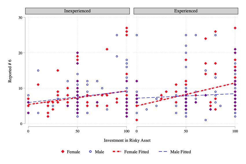
22Figure 3: Correlation between amount invested in risky asset and reported
number of sixes in dishonesty task
Notes: Difference in Slope (female – male) = 0.006 (p-value = 0.125, one sided) for inexperienced
politicians and 0.059 (p-value = 0.011, one sided) for experienced politicians.
game and in the die-tossing game are positively correlated (Figure 3). This correlation
is particularly strong for experienced female politicians.16
The network mechanism
Measuring political networks is challenging, but we try to do this by examining political
connections within the family—as indicating that a politician has access to political
networks even before entering political office. This is operationalized by whether or not
16
The difference in slope (female – male) = 0.006 (p-value = 0.125, one sided) for inexperienced
politicians and 0.059 (p-value = 0.011, one sided) for experienced politicians.
23participants had political leaders in their extended family, elicited in the survey-part of
our study.
To examine whether this mechanism can explain patterns of dishonesty behavior
among inexperienced and experienced politicians, we estimate our model for die-tossing
game separately for politicians with and without dynastic connections. The regression
results are presented in columns 1 and 2 of Table 4. As shown in column 1—and con-
sistent with our theoretical expectations—the difference between inexperienced women
and men in the full sample is driven entirely by the women from non-dynastic families.
Further, the difference between inexperienced and experienced women is much stronger
among those without political connections in the family.
These patterns are consistent with the idea that, because of their weaker political
networks, most women have fewer opportunities than men to act in a corrupt manner,
but that this changes as they gain political experience.
The aspirations mechanism
A fourth possible mechanism for the changing gender gap in dishonesty concerns differ-
ences in aspirations for a future role in politics. If women have lower political aspirations,
they may be more attracted to extracting short-term gains from office. To examine this
mechanism, we asked participants whether they aspired to stand for political office in
the future. Figure 4 shows the average proportion who responded “yes” to aspiring to
stand for any of the following positions: same as current, Pradhan, member of Pan-
chayat Samiti (taluk or block level), member of Zila Parishad (district level), Member
of Legislative Assembly (MLA, state level) or Member of Parliament. We find no gender
difference in aspirations for future political office among experienced or inexperienced
politicians, although both male and female inexperienced politicians report significantly
higher aspirations for future political office than do their experienced counterparts.
24Table 4: Time in Office and Dishonesty. Political Dynasty and
Aspirations
Political Dynasty Future Political Aspirations
No Yes No Yes
(1) (2) (3) (4)
Experienced 0.869 1.077 0.995 1.912*
(0.971) (1.726) (1.709) (1.021)
Female -1.416 0.501 -0.507 -0.782
(0.962) (1.507) (2.511) (0.914)
Experienced × Female 1.961 0.135 0.696 0.658
(1.273) (1.646) (2.415) (1.205)
Constant 11.204*** 10.360*** 13.058*** 9.775***
(2.361) (2.460) (4.381) (2.169)
Sample Size 302 98 104 296
Difference Estimates:
Inexp Female – Inexp Male -1.416 0.501 -0.507 -0.782
(0.962) (1.507) (2.511) (0.914)
Exp Female – Exp Male 0.545 0.636 0.189 -0.124
(1.158) (1.484) (1.938) (1.052)
Exp Female – Inexp Female 2.830** 1.211 1.691 2.571***
(1.113) (1.330) (1.943) (0.975)
Exp Male – Inexp Male 0.869 1.077 0.995 1.912*
(0.971) (1.726) (1.709) (1.021)
Notes: Dependent variable: Reported # of 6’s. OLS regression results presented.
Regressions control for a set of individual characteristics (age, years of schooling,
religion/caste, land owned, political network, primary occupation and party affiliation.
Standard errors clustered at the GP level. Significance:∗∗∗ p < 0.01;∗∗ p < 0.05;∗ p <
0.1.
The pattern in Figure 4 suggests that changing aspirations cannot account for the
time-in-office effect on women’s dishonesty, unless how aspirations and time horizons
affect dishonesty are different for women and men. To examine that possibility, we
estimate our die-tossing model separately for those with and without further political
aspirations.
The results are presented in columns 3 and 4 of Table 4. Although there is clear
evidence of a shorter time-horizon being associated with more dishonest behavior (note
the sizeable constant term in column 3), and also large differences between inexperienced
and experienced politicians, both male and female politicians become more dishonest
25Figure 4: Aspiration for political office in the future
Notes: Bars show the average proportion of politicians in the four categories (inexperienced male, inex-
perienced female, experienced male and experienced female) responding yes to aspiring to stand for any of
the following positions: same as current, pradhan, member of panchayat samiti, member of zila parishad,
MLA, MP.
with time in office. The aspirations mechanism does not seem to explain why women in
particular become more dishonest with time in office.
5 Concluding discussion
Increasing the share of women in politics has been promoted as a way of reducing
corruption and curtailing dishonest behavior. However, relatively little is known about
why and under what circumstances women are more honest and less corrupt than men.
Among ordinary members of the public, women have been found to be more altruistic
26and honest, at least in industrialized countries. However, it requires a considerable leap
of faith to argue that a similar behavioral pattern should be expected among elected
women politicians around the world; likewise with the assumption that gender gaps in
attitudes and behavior will remain static as newly elected representatives gain experience
and become socialized into heterogeneous and localized political cultures.
Our study contributes to the debate on the gender gap in dishonesty by arguing
that this gap should be theorized and studied as dynamic rather than static. There are
differences between men and women in all societies—but if these differences are due to
experiences and socialization, and not inherent traits, they must be recognized as both
context-specific and malleable. Women may be less prone to corruption when they enter
politics, but exposure to the political game, particularly the normalization of corrupt
behavior, is likely to change them. Our study from West Bengal suggests precisely this:
that women who enter politics are somewhat less likely to engage in corrupt behavior
than men, but that they become more likely to do so with time in office—and this seems
to be because of a reduction in risk aversion and stronger political networks.
How generalizable are these results? Our argument implies that gender gaps in
corrupt behavior, and also other forms of political activity, result from differences in
experiences and socialization. The differences between men and women (or other groups)
may not be so great if the lives of men and of women do not differ greatly—or, inversely,
in a society with greater gender gaps, greater differences might be expected between
men and women entering politics.
Further, the greater the difference in culture inside and outside of politics, the more
likely are changes among both men and women as they gain political experience. In
this study of village-level politics in India, we expect scant cultural change for men who
enter politics, as they are often already embedded in the political discourse in their
27villages, whereas entering “the game” at a different level of politics may result in more
of a change among men as well.
With greater gender differences within politics—for example, women experiencing
more hostility—the trajectories of women and men can be expected to differ. In India,
evidence suggests that women’s experiences of politics are worse than those for men.
Although our measures of pro-sociality and trust do not capture such changes, they
cannot be ruled out. More research is needed to establish whether there is evidence of
a shrinking gender gap as men and women become socialized into the same political
environment, or whether exposure to the political game makes women more dishonest
than their male colleagues. Regardless, our study of real-life politicians lends little
support to the idea that women’s entry into political institutions will help clean out
corruption or other malfeasance—except, perhaps, briefly.
References
Afridi, F., V. Iversen and M. Sharan. 2017. “Women political leaders, corruption and
learning: Evidence from a large public program in India.” Economic Development and
Cultural Change 66(1):1–30.
Alatas, Vivi, Lisa Cameron, Ananish Chaudhuri, Nisvan Erkal and Lata Gangadharan.
2009. “Gender, culture, and corruption: Insights from an experimental analysis.”
Southern Economic Journal pp. 663–680.
Ashraf, N., I. Bohnet and N. Piankov. 2006. “Decomposing trust and trustworthiness.”
Experimental Economics 9(3):193–208.
Banerjee, R., T. Baul and T. Rosenblat. 2015. “On self-selection of the corrupt into the
public sector.” Economics Letters 127:43 – 46.
Bardhan, Pranab, Dilip Mookherjee and Monica Parra Torrado. 2005. “Impact of reser-
vations of panchayat pradhans on targeting in West Bengal.” University of California
at Berkeley, Department of Economics, typescript.
Barnes, Tiffany D and Emily Beaulieu. 2019. “Women politicians, institutions, and
perceptions of corruption.” Comparative Political Studies 52(1):134–167.
Baskaran, Thushyanthan, Sonia R Bhalotra, Brian K Min and Yogesh Uppal. 2018.
“Women legislators and economic performance.” WIDER Working Paper 47/2018.
28You can also read