Towards Accountability in Machine Learning Applications: A System-Testing Approach - DISCUSSION PAPER
←
→
Page content transcription
If your browser does not render page correctly, please read the page content below
// NO.22-001 | 01/2022

DISCUSSION
     PAPER
   // WAYNE XINWEI WAN AND THIES LINDENTHAL

Towards Accountability in
Machine Learning Applications:
A System-Testing Approach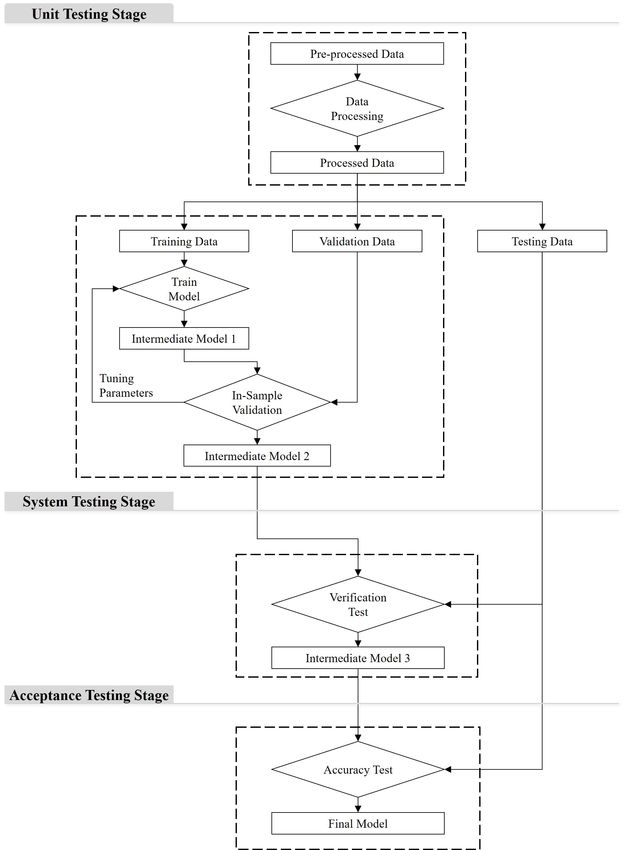
Towards Accountability in Machine Learning
             Applications: A System-Testing Approach

                            Wayne Xinwei Wan*, Thies Lindenthal†

                                           January 4, 2022

                                                 Abstract

 A rapidly expanding universe of technology-focused startups is trying to change and improve the
way real estate markets operate. The undisputed predictive power of machine learning (ML) mod-
els often plays a crucial role in the ‘disruption’ of traditional processes. However, an accountability
gap prevails: How do the models arrive at their predictions? Do they do what we hope they do –
or are corners cut?
     Training ML models is a software development process at heart. We suggest to follow a ded-
icated software testing framework and to verify that the ML model performs as intended. Illus-
tratively, we augment two ML image classifiers with a system testing procedure based on local
interpretable model-agnostic explanation (LIME) techniques. Analyzing the classifications sheds
light on some of the factors that determine the behavior of the systems.

Keywords: machine learning, accountability gap, computer vision, real estate, urban studies

JEL Codes: C52, R30

   * CorrespondingAuthor. Department of Land Economy, The University of Cambridge. Email: xw357@cam.ac.uk
   †
    Department of Land Economy, The University of Cambridge. Email: htl24@cam.ac.uk.

Acknowledgements: This publication is the result of a project sponsored within the scope of the SEEK research
programme which was carried out in cooperation between the University of Cambridge and ZEW – Leibniz-Zentrum
für Europäische Wirtschaftsforschung GmbH Mannheim, Germany. We thank Peter Buchmann for setting up the
infrastructure and providing excellent technical support.
1    Introduction

This paper does not develop any narrowly defined machine learning (ML) wizardry but addresses
a fundamental problem of complex prediction systems: How can we verify that a system is per-
forming in the way it is meant to perform? Can we be sure that its outcomes are not spurious or
biased?
    The triumph of ML applications has only started but has revolutionized commerce, personal in-
teractions, entertainment, medicine, government services, state supervision – and research, already
(Simester et al., 2020). In real estate and urban studies, a rapidly expanding literature explores the
potential of ML algorithms, introducing novel measurements of the physical environments or us-
ing these estimates to improve the traditional real estate valuation and urban planning processes
(Glaeser et al., 2018; Johnson et al., 2020; Karimi et al., 2019; Lindenthal & Johnson, 2021; Liu
et al., 2017; Rossetti et al., 2019; Schmidt & Lindenthal, 2020; Shen & Ross, 2020). These studies,
again and again, demonstrate the undisputed power of ML-systems as prediction machines. Still,
it remains difficult for researchers to establish causality or for end-users to understand the internal
workings of any models. An “accountability gap” (Adadi & Berrada, 2018) remains: How do the
models arrive at their prediction results? Can we trust them not to bend rules or to cut corners?
    This accountability gap holds back the deployment of ML-enabled systems in real-life situa-
tions (Ibrahim et al., 2020; Krause, 2019). If system engineers cannot observe the inner workings
of the models, how can they guarantee reliable outcomes? Further, the accountability gap also
leads to obvious dangers: Flaws in prediction machines are not easily discernible by classic cross-
validation approaches (Ribeiro et al., 2016). More importantly, the opacity of the ML models
also gives rise to the legal and ethical concerns for its real-life applications (Mullainathan & Ober-
meyer, 2017). For instance, anecdotal evidence reports that some ML engines for recruitment have
exerted biases again the female applicants (Dastin, 2018). Traditional ML model validation met-
rics such as the magnitude of prediction errors or F1 -scores can evaluate the models’ predictive
performance, but they provide limited insights for addressing the accountability gap.
    Training ML models is a software development process at heart. We posit that ML system

                                                  1
developers therefore should follow best practices and industry-standards in software testing. Par-
ticularly, the system testing stage of software test regimes is essential: It verifies whether an in-
tegrated system performs the exact function as required in the initial design (Ammann & Offutt,
2016). For ML applications, this system testing stage can help to close the accountability gap
and to improve the trustworthiness of the resulting models. After all, thorough system testing has
verified that the system is not veering off into dangerous terrain but stays on the pre-defined path.
System testing should be conducted before evaluating the model’s prediction accuracy, which can
be considered as the acceptance testing stage in the software testing framework. Accuracy is not
meaningful without verification. Alternatively, the system testing stage could be implemented as a
set of constraints imposed on the model during the training phase.
   Interpreting the mechanism of ML models in the system testing stage is fundamentally chal-
lenging due to the trade-off between the model’s interpretability and flexibility (James et al., 2013),
especially for the deep learning models (LeCun et al., 2015). Earlier methods include visualizing
intermediate activation layers of the input data or the filters in the model (Zeiler & Fergus, 2014),
but understanding the visualizations from these methods are difficult for the end-users. In recent
years, several up-to-date model interpretation algorithms have been developed, which attempt to
reduce the complexity by providing an individual explanation that solely justifies the prediction
result for one specific instance (Lei et al., 2018; Lundberg & Lee, 2017; Selvaraju et al., 2017;
Ribeiro et al., 2016). This kind of model interpretation technique is also referred to as the local
model explanation (Adadi & Berrada, 2018; Molnar, 2019). However, most of the current local
interpretation tools are qualitative and require human inspection for each observation. Thus, these
tools for model verification do not easily scale up with a large sample.
   Examples are often more informative than a long treatise. In this paper, we develop system-
testing stages for two ML-enabled use cases: 1) a building vintage classifier and 2) an automatic
valuation model (AVM) for residential real estate. Both use cases leverage street-level images of
residential real estate as inputs, which are easy to motivate and have been employed in research
recently (Law et al., 2019; Lindenthal & Johnson, 2021). In this paper, we do not have an intrinsic

                                                  2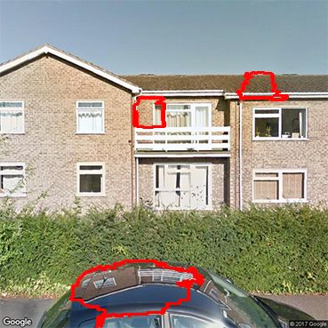
interest in the actual predictions these machines produce but focus on model verification tests:
First, we form expectations on relevant information in the images that the models should pick up
and irrelevant aspects to be ignored, ideally. Then we identify the areas of the input images that
are most relevant for the ML models using a local model interpretation algorithm. The final step
tests whether the models meet the expectations.
    Specifically, we combine expert domain knowledge and an ensemble of ML applications, in-
cluding computer-vision object detection models, image classifiers, and local interpretable model-
agnostic explanation algorithms. We start by asking architects which aspects of a façade they
focus on when trying to assess the vintage of a house. They advise that doors, windows, roof
shape, building materials, proportions, and ratios, or the existence of garages and driveways are
most informative when assessing a house’s vintage, while trees or cars should be ignored. Estate
agents, however, appreciate additional cues such as trees or (expensive) cars when assessing the
value of a home. To them, they are indicators of externalities and a neighborhood’s affluence. We
expect that well-behaved ML models will arrive at similar priorities when analyzing images of
houses.
    Next, we augment off-the-shelf image classifiers that have been re-trained to detect architec-
tural styles of English homes (replicating Lindenthal & Johnson, 2021) or the quintile of price
regression residuals.1 Widely available object detection models can reliably locate doors, win-
dows, overall façades, trees, and cars, among many other object categories. Further, we implement
the local interpretable model-agnostic explanation algorithm (LIME) – one of the popular local
model interpretation tools – to find the areas in the input images that are most relevant for the
predictions.
    Our results reveal that the ML classifiers lay their eyes on the right things. The vintage classifier
indeed focuses on windows and doors and puts less weight on information from the trees and cars.
Classifiers that assess home value, however, have a slightly different way of reading the images.

    1
      A computer-vision based classifier is selected as an illustration due to its popularity in real estate and urban
studies (Naik et al., 2016), although our approach also extends to other ML classifiers, e.g. in text-mining (Ambrose
et al., 2020; Fan et al., forthcoming; Shen & Ross, 2020).

                                                          3
First, the computer vision capabilities of AVM we investigate can capture otherwise unobservable
hedonic housing characteristics and thereby improve the model’s predictive power. To do so, the
classifier embedded in the AVM pays attention to informative objects like doors and windows,
just like the vintage classifier before. More interestingly, however, the AVM will rely more on
indirect cues of value such as cars, just as we hoped. In sum, we can confirm that our ML black
box examples do not venture far away from what a true expert would do – that peace of mind
is the true contribution of this paper.2 Overall, we do not aim for internal or external validity in
a typically applied economics sense. Instead, we promote a conceptual terminology and offer a
proof of concept – an approach often found in engineering or computer science papers.
   In addition, we extend the existing qualitative model-interpretation techniques to a formal
quantitative test. Methodology-wise, this helps to scale up the model interpretation analyses for a
large sample size, which is essential for most of the applications in real estate and urban studies.
In summary, our proposed method extends to other ML models and, due to the essence of closing
the accountability gap, this study has important implications for ML applications in real estate and
urban studies, as well as in other subjects beyond.
   Due to the nature of local model interpretation, the design of system testing is specific to
the functional requirement of the models. Therefore, we also discuss a few factors that need to
be considered when designing a system test. Firstly, we find that, with a larger size of training
samples, the system testing scores saturate earlier than the prediction accuracy scores. Secondly,
the appropriate size of the selected interpretable information is essential for reaching a reliable
system testing score. Lastly, the quality of the input training data (i.e. the noise level) also greatly
impacts the model’s performance in the system testing.
   The rest of the paper is structured as follows. Section 2 reviews the literature that applies ML
models, particularly the image-based ML classifiers, in real estate and urban studies. Section 3
describes our proposed system testing approach and suggest a model verification test. Section 4
illustrates the suggested system testing stage with two concrete examples of ML systems, and the

   2
       Depending on the use case, additional tests might be advisable for a full due diligence, of course.

                                                            4
system testing results are presented in Section 5. Section 6 discusses some practical factors that
impact the performance of the system tests. Section 7 concludes.

2    Literature Review

Over the past few years, the application of ML techniques in evaluating human perceptions of
housing quality and urban environment has caught increasing attention in the literature (Aubry
et al., 2019; Koch et al., 2019). For example, the studies on the aesthetic value of residential
properties demonstrate how the predictive power of ML models improves the traditional real estate
valuation process. Before the wide application of ML methods, some literature has provided clues
that the aesthetics of different architectural styles carry impacts on the market transaction price
(Buitelaar & Schilder, 2017; Coulson & McMillen, 2008; Francke & van de Minne, 2017). The
exteriors of a building also introduce externalities that can spill over to the market price of sur-
rounding buildings (Ahlfeldt & Mastro, 2012; Lindenthal, 2017). Nevertheless, a majority of these
prior studies using traditional approaches, such as the human assessment by experts or surveys, to
measure the subjective perceptions towards the physical housing features (Freybote et al., 2016).
The human assessment is normally costly and time-consuming, and it is also threatened by the
limited sample size and large bias from unobserved factors. Some other studies use indirect mea-
surements of the building styles, such as the zoning of conserved buildings or the introduction of
redevelopment projects, to achieve cleaner institutional settings for the evaluation (Ahlfeldt et al.,
2017). Unfortunately, few of these approaches can scale up well.
    Emerging literature aims to address these challenges by applying deep learning techniques to
classify human perceptions towards housing quality. Utilizing the rich building-level images from
Google Street View, Glaeser et al. (2018) find that the improvement in building appearance is
associated with higher home values in Boston, while the appearance of foreclosed properties de-
preciates significantly. In the UK, the architectural style is found to be a significant determinant
for resale prices, but it has a limited impact on the primary market (Lindenthal & Johnson, 2021).

                                                  5
Law et al. (2019) show that street image and satellite image data can capture visual urban qualities
and improve the estimation of house prices. By identifying the uniqueness of building vintages
relative to the surrounding neighborhoods, Schmidt & Lindenthal (2020) document that the behav-
ior of rounding price is linked to the liquidity and uniqueness of assets. Johnson et al. (2020) also
confirm the price premium from a property’s curb appeal, and they discover that the premium is
more pronounced during market downturns. Using ML algorithms to quantify levels of semantic
uniqueness in property descriptions, Shen & Ross (2020) find that the uniqueness of properties
leads to higher prices and longer listing periods.
   Apart from the strength in assessing the quality of individual houses, recent literature has also
demonstrated the power of ML methods in urban studies. It illustrates that the ML methods can ef-
fectively measure many previously unobserved features of the urban environments (Ibrahim et al.,
2020). On the social dimension, several studies reveal that demographics in the neighborhood,
including income, race, education, and voting patterns, are associated with and are predictable
by the physical appearance and perceived safety of the urban environment (Gebru et al., 2017;
Glaeser et al., 2018; Naik et al., 2016, 2017). On the dimension of physical planning, greenery
and street-facing windows are found to positively attribute to the perception of safety (De Nadai
et al., 2016). Rossetti et al. (2019) quantify the quality and human perception of public spaces
in urban environments. Zhang et al. (2018) propose a framework to represent the locale of street
scenes, while Liu et al. (2017) evaluate the maintenance quality of building façade and the sense
of continuity along the streets in Beijing.
   While deploying ML models is getting more popular in the research of housing and urban
environment, a vital concern remains: If the end-users do not understand and trust an ML model,
they will not use it (Ribeiro et al., 2016). This is especially true when we aim to move one step
forward, from the models’ predictions to real-life decisions and policymaking (Ibrahim et al.,
2020). Unfortunately, it is textbook knowledge that there exists a trade-off between a model’s
flexibility (i.e. prediction accuracy) and the model’s interpretability (James et al., 2013). For the
deep learning models that we develop, the nature of complexity hinders end-users from interpreting

                                                     6
them, and the end-users normally just consider the models as “black boxes”. As a result, this
becomes an essential barrier for promoting policy insights from the models’ prediction results.
    To bridge this accountability gap, several model interpretation methodologies have been intro-
duced (Adadi & Berrada, 2018; Lei et al., 2018; Lundberg & Lee, 2017; Selvaraju et al., 2017;
Ribeiro et al., 2016) in recent years. The intuition behind this is that, although the global decision
function of a classification model is very complex and hard to interpretable, justifying the predic-
tion for a specific instance is feasible with fidelity. For instance, Ribeiro et al. (2016) propose
a novel local interpretable model-agnostic explanation (LIME) system to explain ML classifica-
tion models with human-understandable representations by approximating the model locally with
sparse linear explanations.3 The image to be classified is firstly divided into several interpretable
components (i.e., contiguous super-pixels). Then, by randomly turning some of the super-pixels
off, the algorithm generates a set of pseudo instances “near” the original image and tests how the
classification result of each pseudo instance deviates from the classification of the original image.
Finally, by learning a locally weighted linear model on the pseudo instances, the super-pixels with
the highest positive impact on the initial classification are selected as the explanation of the model.
More recently, Lundberg & Lee (2017) proposed the Shapley Additive Explanations (SHAP) for
the local interpretation of models. Instead of using linear regression as in LIME, this method
weights each feature using the Shapley value originated from game theory. It is worth noting that
these methodologies are qualitative, and each explanation is only valid for one local instance (i.e.,
each specific image). One exception is the recent study by Krause (2019), which uses the model-
diagnostic method to extract the marginal contribution of each period toward observed prices in
the data and then constructs a house price index, accordingly.
    In addition to the challenge of low interpretability, the unopened “black box” may also lead to
undesirable classifiers, in which the model’s flaws are very difficult to be identified if we merely
check the accuracy of prediction. Ribeiro et al. (2016) demonstrate this modeling issue with an
experiment classifying the photos of wolves and huskies (see Appendix Figure A2). They in-

    3
      Appendix Figure A1 visualizes the intuition of LIME using a classification function in a 2-D panel. See Ribeiro
et al. (2016) for detailed discussions.

                                                         7
tentionally choose pictures of wolves that have snow in the background, and pictures of huskies
without snow, as the training samples. As a result, the trained classifier predicts “wolves” based
on the snow in the background rather than the animals. However, this flaw in the model cannot be
easily identified by just reviewing the prediction accuracy, especially if all the images of wolves in
the validation test have snow in the background.
   As a result, we argue that the standard metrics testing the prediction accuracy of an ML
model—such as the F1 score and the Herfindahl index— are not sufficient to evaluate the model’s
performance. Lindenthal & Johnson (2021) also discuss this potential misclassification issue,
specifically in the context of housing quality and urban environments. They find that the automat-
ically collected street images contain irrelevant information like trees and vehicles for classifying
building vintages. Images with larger areas showing the buildings will result in higher classifica-
tion accuracy. However, there is still no direct evidence showing whether the model has included
irrelevant information in the predictions.
   To close these research gaps, we extend the qualitative local model-explanation method in the
prior literature to a formalized quantitative evaluation method in this study, denoted as a model ver-
ification test. In addition, using a concept similar to the testing procedures in software development
(Ammann & Offutt, 2016), we propose an extended testing framework for the general ML models
in real estate and urban studies. Given our model verification test is not restricted to the types of
classification problems or the exact ML algorithms chosen, we use a model with deep networks for
image classification as our illustrative example, which is one of the most popular ML applications
for researches in housing quality and urban environment. Also, we choose to implement one of the
commonly used local model interpretation techniques—the LIME algorithm proposed by Ribeiro
et al. (2016)—in the paper, while the other model local interpretation methodologies like SHAP
also apply for our testing approach.

                                                   8
3 System Testing and Model Verification Tests
This section first proposes an abstract framework of system testing that improves the interpretabil-
ity and due diligence of ML models. Subsequently, it describes a concrete system testing im-
plementation based on a quantitative model verification test suitable for ML models using image
data.
3.1 System Testing
A dedicated testing framework has been widely adopted in software engineering (Ammann &
Offutt, 2016): To ensure that functionality and performance meet the pre-specified requirements,
the newly developed software usually needs to pass four major stages of testing before deployment.
The unit testing stage examines the functionality of individual components of the software; the
integration testing stage examines whether the individual units are well combined; the system
testing stage checks whether the integrated system meets all end-to-end specifications. In the last
step, then the acceptance testing stage assesses the performance of the system to ensure acceptance
by end-users.
The processes of developing ML models can also be generalized using the same concepts from
software development. Data collection and pre-processing can be considered as separate functional
components that could be verified with empirical unit tests. Depending on the complexity of the
research questions, one or more ML models might be trained, and each trained model can again
be considered as a separate functional unit, which can be tested by means of in-sample cross-
validation. The frequently-used ML model accuracy tests assess whether the performance (i.e.
prediction accuracy) of the system meets the end user’s requirements, similar to an acceptance
test.
Missing, however, is a system-testing stage to ensure that the integrated system of the func-
tional units performs as intended and that the predictions are obtained reliably.4 Following best
4
More accurately, there are more than 50 types of system testing for various purposes. Investigating whether the
model performs the exact function as required is more similar to our proposed concept of functional testing, which is
a critical one among these system tests. See Ammann & Offutt (2016) for detailed discussions.
9Figure 1: The Flow Chart of Machine Learning Process with the Proposed System Testing
Notes: The figure plots the flow chart of our proposed framework for applying machine learning models in real estate
and urban studies. Using the concept similar to the hierarchies of system testings, we consider data collection and
each trained models as individual units. For simplicity, only one trained model is plotted in this flow chart, and the
integration testing between the units is ignored. The classic accuracy test is considered as the acceptance testing of the
model. Our proposed model verification test is considered as a system testing to investigate whether the model serves
the initial functional purpose as expected, and it is conducted before the acceptance testing.
10practice, we argue that system tests of any ML system should be successfully passed before even
starting to verify the model’s predictive performance.
3.2 Model Verification Test for (some) CV Models
While system testing is a conceptual stage to verify that ML models comply with the design re-
quirements, specific testing routines, so-called model verification test, are needed to conduct this
stage. Next, we design a novel model verification test and demonstrate how to implement system
testing for one of the major applications of ML models in real estate and urban studies – ML im-
age classifiers (Glaeser et al., 2018; Johnson et al., 2020; Liu et al., 2017; Rossetti et al., 2019;
Schmidt & Lindenthal, 2020; Lindenthal & Johnson, 2021).
Obviously, a concrete implementation of a system test depends on the specific task at hand, the
data used and the type of models trained. Here, we suggest not peak into the inner workings of
ML systems directly but instead to analyze whether model outcomes can be traced back to input
characteristics. To do so, we leverage relatively new local model interpretation techniques that
reveal the elements or aspects of input data that are most decisive for a model’s output. We then
determine how much of this crucial information overlaps with desirable information, based on
human expert input.5
More specifically, our model verification test suits the situation when we classify images j
into different categories (e.g., classify building into architectural styles, uniqueness levels, price
ranges, etc.), and we want to understand whether the ML models have used information of object
i (e.g., building façades) for the classification. The model verification test returns two quantitative
testing outputs—the verification test score and ratio, which both measure to what extent that the
ML model uses information i for the classification results.
Firstly, we calculate the model verification test score (T estS corei j ) for each object type i in
5
A fundamentally different alternative, a so-called global model interpretation approach, investigates the func-
tionality of individual components “inside” ML models, e.g., the neurons in a deep convolution neural network model
(Olah et al., 2020). However, due to the complexity in global interpretation, these tools normally require strong as-
sumptions on the explainable functionalities (Zeiler & Fergus, 2014). To use another neurological metaphor: The
global model interpretation approaches are comparable to MRI scans that try to detect and explain patterns of activity
in human brains.
11the image j. This score represents how much the model predicts based on the information from
object type i in this image j. Technically, we first extract object i in an image j, using the off-
the-shelf ML object detection tools. For a specific object i, we denote the associated area in the
image as Ob jectAreai j . There may exist multiple objects in this object type, and we denote the
set of all these objects as I. Next, we analyze which areas in the images (i.e., the super-pixels)
contribute the most to the model’s classification decision, using local interpretation tools such as
the LIME algorithm. We call the area of the image j that best explaining the classification result
“the interpretable area”, which is denoted as InterpretArea j . The verification test score is then
calculated as follow:
S T
( i∈I Ob jectAreai j ) InterpretArea j
T estS corei j = . (1)
InterpretArea j
We find the overlaps between the interpretable areas and the detected object areas of type i. Since
the sizes of interpretable areas are not equal in every image, we normalize the overlapped area
by the size of the interpretable area. In other words, the test score equals the proportion of the
interpretable areas that originate from the object type i. The interpretation is that, if the test score
is higher, the model utilizes more information from this object type for its predictions. Therefore,
this also marks an advancement in the previous ML interpretation methodology: While the image
segments returned by previous methods help to interpret how the model works qualitatively, we
propose a quantitative approach to formalize the model verification test.
Secondly, we calculate an additional testing output, named as the verification test ratio. We
introduce this alternative testing output because the detected object areas in each image may not
be equal. It is noteworthy that if the model just randomly selects any image segments to make
predictions, the probability that it captures information from objects in type i should equal the total
area of objects in type i divided by the total area of the image. To address this issue, we construct
a benchmark for the verification test score of object i in image j:
S
Ob jectAreai j
i∈I
Benchmarki j = . (2)
ImageArea j
12If the test score is higher than the corresponding benchmark score, it indicates that the model is
intentionally capturing information from this object type to reach the prediction results. Accord-
ingly, we calculate the ratio of the verification test score to the benchmark score to further address
the different scales of benchmark scores across object types:
T estS corei j
T estRatioi j = . (3)
Benchmarki j
The interpretation is that, if the ratio is larger than one, it implies that the model intentionally ex-
tracts information from this type of object for the classification. In contrast, a ratio lower than one
implies that the model considers the information from this object irrelevant for the classification.
4 Two Examples
To illustrate how the proposed model verification test helps to interpret and verify the outcomes of
ML models, we use two common applications of ML in real estate and urban studies as examples.
The first model classifies images of houses, ensembles, or streetscapes into pre-defined categories,
all based on street-level image data (Glaeser et al., 2018; Johnson et al., 2020; Liu et al., 2017;
Rossetti et al., 2019; Schmidt & Lindenthal, 2020; Lindenthal & Johnson, 2021). The second ex-
ample is a basic AVM that combines a traditional hedonic model with a computer vision approach,
again classifying building image data by property value (similar to, e.g., Ahmed & Moustafa,
2016; Law et al., 2019).
4.1 Example 1: Architectural Style Classification
In the first example, we replicate Lindenthal & Johnson (2021) and classify the architectural styles
of residential buildings in Cambridge, UK. The guiding principle for our classifier is to emulate
human experts’ classifications as closely as possible. This implies it should focus on the same
aspects that architects or realtors would pay attention to. The model should...
13• ... focus on the façade of the house and ignore the background, sky, gardens, yards, people,
or streets;
• ... inspect the brickwork, which again is a good indicator for vintage in Cambridge.
• ... pay attention to doors and windows, as their sizes, locations and styles are correlated with
the house’s vintage;
• ... ignore trees and cars as much as possible;
While we do not wish to discard subconsciously picked up cues or patterns, our tests can only
reflect clear rules. A subjective statement such as “this façade somehow reminds me of a Georgian
house I once lived in” might be true but cannot be translated into a test requirement.
4.1.1 The Vintage Classifier
We first replicate the ML vintage classifier in Lindenthal & Johnson (2021) and re-use their exten-
sive image dataset of around 25,000 building images from Cambridge (UK). These images have
been collected from Google Street View and classified into architectural styles by architects.6 To
achieve both a clearer differentiation and a more balanced sample size for each category of the
architecture style, we classify the samples into seven styles, including the Georgian, Early Victo-
rian (denoted as Victorian for short), Late Victorian/Edwardian (denoted as Edwardian for short),
Interwar, Postwar, Contemporary, and Revival style. Appendix C summarizes the definitions and
key features of these architectural styles in the UK.
We conduct stratified sampling by architectural styles to construct the dataset for the model’s
training, in-sample validation, and out-of-sample testing. In total, there are 2,791 buildings se-
lected in our out-of-sample testing dataset. We first use the Inception computer vision models
(Szegedy et al., 2016) to obtain 2048 element strong feature vectors for each image. Then we train
a deep convolutional neural network model to classify buildings into seven architecture styles,
6
This sub-sample is far larger than the required sample size to reach the model’s saturated training accuracy, but
more images are manually tagged with the architectural styles to enable the out-of-sample validation of the model’s
prediction accuracy. See Lindenthal & Johnson (2021) for a detailed discussion.
14which gives us the classification model that we intend to analyze further. The technical details of
training the vintage classifier are provided in Appendix D. The out-of-sample classification perfor-
mance is of secondary interest to us but cross-validation results can be found in Appendix E.
The standard metrics of model prediction accuracy, e.g. precision, recall, F1 scores, or the
Herfindahl index of the scores for each vintage (HHI) indicate that our simple model performs
at a satisfactory level. To better understand the way the model classifies the images, we apply
the LIME model explanation algorithm following Ribeiro et al. (2016) to all images in our test
sample.7 For each image, the algorithm detects the image segments that were most relevant for the
model to classify the house into the most probable style. These areas are called super-pixels. We
limit the number of super-pixel groups the algorithm can identify to a maximum of five.
Finally, our model verification tests all relate to classes of objects that should be in the focus
of the classifiers – or not. We automatically detect façades, doors, windows, trees, or cars on all
the 2,791 images in the testing sample set. To give an example, Figure 2 presents a selection of
objects detected in one randomly selected image.8 A rectangular mask is drawn tightly around
each identified object, and a numerical score is returned denoting the confidence in the detection
result. Admittedly, many objects do not have perfectly rectangular shapes. Still, we consider the
area within the mask as the relevant image area associated with the specific object. A visual check
confirms that our object detection model effectively identifies all objects of interest in our sample
reliably.
4.2 Example 2: AVM Residual Value Classification
The second example is a simple hedonic valuation model that is augmented by an additional ML
building image classifier. The goal is to extract additional information from the residuals of a
hedonic regression by classifying the homes into residual value quintiles using images. Other than
the difference in classification categories, the classifier is identical to the previous example.
7
The package is available at: https://github.com/marcotcr/lime
8
We use the latest version of the Inception/ResNet object detection model: https://github.com/tensorflow/
models/blob/master/research/object_detection/g3doc/detection_model_zoo.md.
15Figure 2: Object Detection in Images
Notes: This figure provides an example of object detection results in our testing image samples. Each detected object
is enclosed by a box, labeled with the classified object type. The corresponding percentage next to the label indicates
the confidence in the detection results.
Again, we analyse whether the super-pixels coincide with doors, windows, or other objects. In
addition, we investigate how the super-pixels will differ when the classification task changes. We
expect some overlap in super-pixels from the architectural style classification and a residual value
classification. Architectural styles have been documented as important determinants of residential
property price in the UK (e.g. Law et al., 2019; Lindenthal & Johnson, 2021) and the residual value
classifier is likely to focus on the same objects as the architectural style classifier. Adding style
information to the hedonic regression stage, however, should reduce the reliance on architectural
features and lead to more different super-pixels.
We form several hypotheses of the model verification testing results for this example:
• There is information in the residuals from the hedonic price model that can be extracted by
the ML image classifier. Adding the residual value classifier will improve the accuracy of
the overall AVM.
• Residual value classifiers will categorize buildings more accurately when residuals stem
16from relatively parsimonious hedonic models. For models with only a few hedonic variables,
there are simply more unobserved factors that might be picked up in the images.
• The super-pixels from the residual value classifier will partially overlap with the superpixels
from the architectural style classification in 4.1. However, the overlap will be smaller when
architectural style is added as a hedonic variable in the initial hedonic regression.
• The residual value classifier will disproportionally rely on information from windows and
doors because windows and doors are critical determinants of building styles.
• Positive externalities from greenery could influence property values. We expect trees to
matter more for residual values than for architectural styles.
• Cars and property value are both related to a household’s wealth. We, therefore, expect
information on nearby cars not to be ignored when trying to assess a house’s value.
4.2.1 AVM Data and Methodology
In this example, we combine the same image data in the first example with the transaction data.
We collect the residential property transactions in Cambridge, England between January 1995 and
October 2018 from the UK Land Registry. The Land Registry records the date of transaction, the
price paid, street address, a classification of the property type (flat, detached, semi-detached, or
terraced house), the estate type (freehold or leasehold), and an indicator for newly built properties.
We exclude the leasehold properties and flats in our sample. This ends up with 26,841 transac-
tions of 15,855 buildings. Appendix Table B1 presents the summary statistics of the transaction
data. We also measure each building’s floor areas using maps for the UK Ordnance Survey and
estimate the building’s volume by combining the building outlines with digital elevation models
from the Environment Agency (2015), following the method by (Lindenthal, 2018). In addition,
we also measure the distance from each residential property to the city center (i.e., the Great St.
Mary’s Church). Lastly, we match the address of the buildings with 69 unique district codes in
17Cambridge.9
Our first hedonic price model without controls for the architectural styles (Model 1) is specified
as follow:
0
log(Priceit ) = α0 + Xit β + ϕt + ωi + it . (4)
log(Priceit ) is the logarithmic form of the transaction price for property i at time t. Xit is a set of
hedonic housing features, including the logarithmic form of distance to the city center, the floor
area, and the volume of the house; and a dummy variable indicating the new constructions. ϕt
and ωi denote the year and district fixed effects, respectively. it is the error term. Our second the
hedonic model (Model 2) is modified from Equation (4) by adding an additional set of dummy
variables denoting the predicted architectural styles from our ML model in Section 3. The coeffi-
cients of the two hedonic models are estimated using the full sample of transactions, excluding the
2,791 buildings in the out-of-sample prediction set. Appendix Table B2 reports the hedonic model
estimation results.
Then, we train the ML models to classify the residuals of the two hedonic models in terms of
five quintiles10 , using the sample of 13,448 building images that can match with the most recent
transaction record (excluding the 2,791 images in the predict sample set). Like our ML model
for classifying architectural style in Section 3, we randomly sampled 80% of these images as the
training data and use the rest 20% as the in-sample validation data. The other model settings are
the same as the architectural style model. Lastly, we use the ML classifiers to predict the hedonic
price residuals (i.e., which quintiles it belongs to) of the sampled images in the prediction set.
9
We classify the districts according the Lower Super Output Areas (LSOA) in the UK, which typically has 1,000-
3,000 residents and 400-1,200 households of comparable economic and socio-demographic characteristics.
10
Images can also be trained to directly predict the continuous residuals of the hedonic price models. Here we
transform to a classification problem to be comparable with results of the architectural style classifications
185 Results
5.1 Example 1: Vintage Classification Based on Street-level Imagery
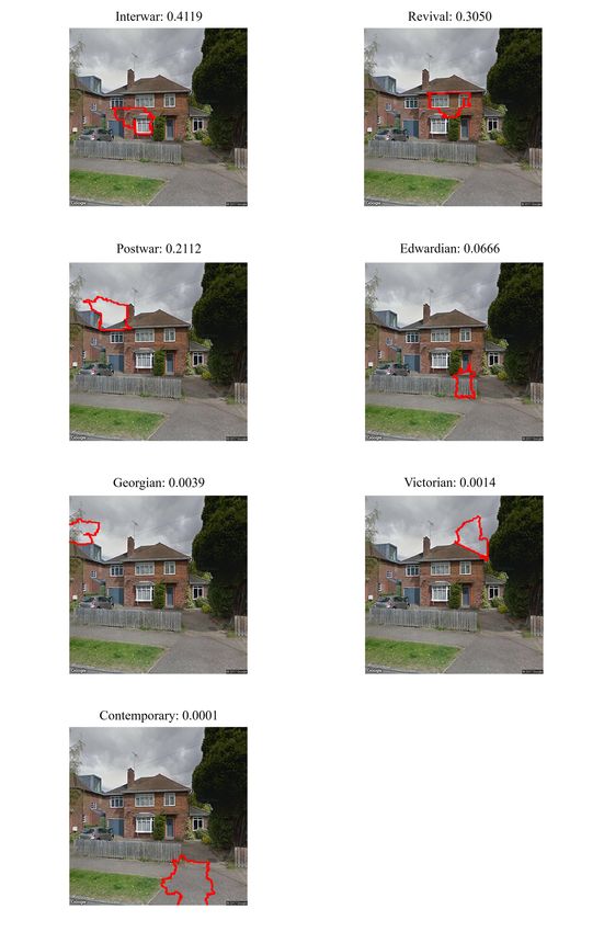
Figure 3 illustrates the interpretation results of an Interwar-style house, which is correctly pre-
dicted by the model with a prediction score of 0.4119. The verification test reveals that the model
has mainly considered the brickworks in the front door and the design of windows on the first
floor for this conclusion. Nevertheless, the model has relatively low confidence in this prediction
result, with the HHI equal to 0.3117. The top second and third predicted styles are Revival and
Postwar, and the corresponding prediction scores are 0.3050 and 0.2112, respectively. The most
decisive building features for these incorrect predictions are the windows on the second floor and
the sloping roof. In contrast, the model has effectively distinguished this building from the other
four building styles, because the corresponding prediction scores are all lower than 0.1. Interest-
ingly, the LIME analysis reveals that only some irrelevant information in the image—such as the
sky, the fence of the garden, and the road—may potentially “explain” these four incorrect styles.
In other words, the model does not establish associations between any physical features of this
house and the four incorrect styles, which further supports that the model has confidently rejected
these four styles based on the relevant information.
Apart from improving the model’s trustworthiness by interpreting the associations with relevant
information, it is also important to assure that the model does not capture the irrelevant information
to reach the correct classifications by coincidence. Figure 4 shows two examples of the analysis
results. The Edwardian-style building in Figure 4a is correctly classified by our model. The
analysis shows that this prediction is mostly based on the brick patterns and sash windows, which
are the key features of Edwardian buildings. However, in a much smaller number of cases, we find
the model’s prediction is also influenced by irrelevant information, even though the final prediction
result turns out to be correct coincidentally. Figure 4b shows a Postwar-style building that is also
correctly classified by the model. However, the model classifies this image mainly based on the
top of a black car, which just accidentally passes by the building.
19Figure 3: Interpretation for the Model’s Prediction Scores on Each Architecture Style
Notes: This figure shows the local model interpretation results for an interwar-styled building, which is correctly
classified by the model but with low confidence (HHI = 0.3117). The model’s prediction score for each architectural
style is reported, which denotes the probability that the building belongs to the corresponding style. The images show
the most decisive super-pixels that explain each architectural style.
20Figure 4: Interpretation for the Classifier’s Ability of Capturing Relevant Information
(a) Relevant Information
(b) Irrelevant Information
Notes: Figure (a) is an Edwardian-styled building that is correctly classified by the model. The local model interpreta-
tion analysis shows that the model captures the relevant information of the bricks and sash windows for this prediction.
Figure (b) shows a postwar building that is also correctly classified by the model. However, the model classifies this
image mainly based on the top of a black car, which accidentally passes by.
21The previous visual inspection is only the interpretation for each input instance, and it does
not easily scale up in the context of big data. Thus, we formalize the inspection by calculating
the proposed verification test score of each image. As described in our hypothesis (Section 4.2),
we use the test score for houses—the most essential objects for classifying building styles—as
the baseline result, and we use the test scores for windows and doors as the robustness checks to
address the concern that some pictures only capture parts of the buildings. We also calculate the
test score for trees and cars as the indicators for capturing irrelevant information.
Panel A of Table 1 reports the average verification test scores for the sub-samples of each
building style. For the classification of Georgian, Victorian, Edwardian, or Revival buildings, the
verification test scores of houses range from 0.857 to 0.890, which indicates that the model well
captures the housing features for the classification of these building types. Similar patterns are
observed if we use the verification test scores of windows or doors as alternative measurements.
For the Edwardian-style buildings, the verification test score for windows is as high as 0.302,
which affirms the finding in Figure 4a that the model captures the unique design of windows for
this architectural style. However, for the classification of Postwar-style buildings, only 69% of the
most explainable areas are from the houses. This is also a support for the unique case we observe
in Figure 4b that the irrelevant information may threaten the trustfulness in classifying Postwar-
style buildings. To further eliminate the potential bias from images showing the only parts of the
buildings (i.e., the verification test score of house in these images will always be one), we exclude
these samples in an additional robustness check and report the updated verification test scores in
Appendix Table B3. Similar trends are observed, which indicates that our main conclusions are
robust.
One major concern of the proposed verification test score is that the areas of objects in each
image are not equal. To address this issue, we first compare the test scores with the benchmark
score—the percentages of the objects’ areas in the images, which are reported in Appendix Table
B4. The model verification scores of houses are all larger than the benchmark score. This assures
that the model is trustworthy because it is intentionally capturing information from the houses for
22Table 1: Verification Test Results of Vintage Classifier
Panel A. Verification Test Score
Architect’s Classification
(1) (2) (3) (4) (5) (6) (7) (8)
All Georgian Victorian Edwardian Interwar Postwar Contemp. Revival
House 0.801 0.857 0.890 0.874 0.779 0.690 0.728 0.888
(0.005) (0.029) (0.008) (0.009) (0.010) (0.012) (0.013) (0.012)
Window 0.188 0.241 0.176 0.302 0.187 0.136 0.137 0.178
(0.004) (0.029) (0.008) (0.010) (0.008) (0.007) (0.007) (0.010)
Door 0.036 0.071 0.081 0.045 0.011 0.010 0.031 0.029
(0.002) (0.019) (0.006) (0.005) (0.002) (0.003) (0.004) (0.005)
Tree 0.093 0.082 0.030 0.083 0.143 0.130 0.085 0.078
(0.004) (0.027) (0.005) (0.008) (0.010) (0.010) (0.009) (0.011)
Car 0.052 0.005 0.074 0.053 0.052 0.049 0.042 0.045
(0.002) (0.004) (0.007) (0.006) (0.006) (0.006) (0.005) (0.008)
Panel B. Verification Test Ratio (Verification Test Score/Benchmark)
Architect’s Classification
(1) (2) (3) (4) (5) (6) (7) (8)
All Georgian Victorian Edwardian Interwar Postwar Contemp. Revival
House 1.103 1.114 1.068 1.127 1.140 1.080 1.061 1.176
Window 1.336 1.493 1.024 1.581 1.524 1.414 1.081 1.441
Door 1.399 1.765 1.515 1.406 1.062 1.579 1.211 1.304
Tree 0.787 0.774 0.769 0.701 0.782 0.764 0.985 0.760
Car 1.167 2.065 1.359 1.181 1.126 1.248 0.968 0.992
Notes: In Panel A, the verification test score presents the proportion of the interpretable area (super-pixels) that overlap
with objects detected in the image (e.g., house or window), by vintage. Standard errors are reported in parentheses. In
Panel B, the verification test ratio normalizes the verification test scores by dividing by the share each object takes up
of the entire image. A ratio larger than 1 means that the ML model uses relatively much information from the object
type to classify building styles, a score below 1 indicates a lack of emphasis. The ratios for the façade, windows, and
doors are larger than 1 overall, lower than 1 for trees, and mixed for cars.
23the predictions. Taking a closer look at each category, it is questionable whether the low test score
is driven by the low proportion of buildings in the images. For the Postwar category, the area of
buildings on average only constitutes 63.9% of the image area in the testing data, which implies
more noises and thus increases the difficulty of classification.
We further calculated the ratio of our verification test score to the benchmark, which is denoted
as the verification test ratio. The results are reported in Panel B of Table 1. This ratio represents
the effort that the model selects information from that type of object, in comparison with randomly
selecting information from the image. After controlling for this heterogeneity in the testing data,
the test ratio of the postwar building is still relatively low at 1.08 and the test ratio for Edwardian
buildings is still the highest at 1.127. For all the seven building styles, our model intentionally
selects the relevant information from houses, windows, and doors, because these test ratios are
larger than one. In contrast, the model also disregards irrelevant information from the trees as we
hope, because the ratio is lower than one.
One interesting finding is that the model also captures information from cars for the classifi-
cation of several building categories, as those verification test ratios are larger than 1. When we
initially design the verification test, we consider that cars are irrelevant to the building vintages.
However, it is plausible that cars are not really “irrelevant” information due to endogeneity: The
architectural styles may correlate with some other specific designs (i.e. large spaces in the front
door), which allow cars to be parked in front of the buildings. Unobserved factors like the demo-
graphics and wealth status of homeowners may also both correlate with the type of their cars and
the architectural style of their homes (Bricker et al., 2020).
To answer this question, we further test the impact of capturing information from each category
on the model’s prediction accuracy. The hypothesis is that, if the model captures more real relevant
information from the training samples, it will have a higher prediction accuracy in the testing
samples. In other words, if capturing information from cars decreases the model’s classification
accuracy, we can reject the hypothesis that unobserved correlation exists between cars and building
styles, and we can be affirmed that the cars are irrelevant information.
24We first examine this hypothesis using a univariate t-test, of which the results are reported in
Table 2. Specifically, we compare the means of verification test scores between the correctly and
the incorrectly classified images. It reveals that, in the correct classifications, the model relies more
on relevant information like houses, windows, and doors, and it captures less irrelevant information
about trees and cars. All the differences in mean are statistically different at the level of 1%. The
results remain robust if we compare the difference in mean using sub-samples of each category
(Appendix Table B5).
Table 2: Verification and Accuracy of Vintage Classifier - Univariate Test
(1) (2) (3)
Y: Verification Test Score
Correct Classifications Incorrect Classifications Difference (1)-(2)
House 0.8186 0.7624 0.0562***
(0.0052) (0.0093) (0.0107)
Window 0.1984 0.1640 0.0344***
(0.0042) (0.0064) (0.0077)
Door 0.0392 0.0271 0.0121***
(0.0024) (0.0029) (0.0038)
Tree 0.0853 0.1095 -0.0242***
(0.0042) (0.0073) (0.0084)
Car 0.0485 0.0609 -0.0123**
(0.0028) (0.0050) (0.0057)
Notes: This table compares the verification test scores for the subsample of correct classifications and incorrect
classifications. A higher verification test score for an object type means that the ML model uses more information
from the object for classification. Column (1) reports the model verification score for the correctly classified sample.
Column (2) reports the model verification score for the incorrectly classified sample. A positive difference in Column
(3) means that the ML model uses more information of the object (e.g., house) for the correct predictions than for the
incorrect predictions, and vice versa. Standard errors are reported in parentheses. *** pof house increase by 0.1, the odds ratio of a correct classification will increase by approximately
0.058 (Column (1)) to 0.074 (Column (2)), and these estimates are statistically significant at the
level of 1%. Similarly, the odds ratio improves with higher verification test scores of windows
and doors, and it decreases with higher verification test scores of cars and trees. Since capturing
information on cars is not associated with higher classification accuracy, it implies that cars are ir-
relevant information as we originally hypothesized, and we should adjust the model from capturing
information of cars.
Table 3: Verification and Accuracy of Vintage Classifier - Logit Regression
(1) (2)
Y: Correct Classification (Yes = 1)
House 0.5832*** 0.7445***
(0.1883) (0.1994)
Window 0.6105** 0.6910**
(0.2744) (0.3042)
Door 0.8968* 0.8705*
(0.4878) (0.5048)
Tree -0.4670** -0.4726**
(0.2064) (0.2109)
Car -0.2696 -0.2358
(0.3132) (0.3186)
Building Style Fixed Effect N Y
Observations 2,791 2,791
Pseudo R-Squared 0.014 0.027
Notes: This table presents logit regression estimates for the impact of verification test scores on prediction accuracy.
The dependent variable is a binary variable denoting whether the building is correctly classified. The explanatory
variables are the model verification scores for each object of interest. A higher verification test score for an object
type means that the ML model uses more information from the object for classification. A positive estimate of the
coefficient means that a higher verification test score of the object (i.e., using more information from the object for
classification) correlates with a better prediction accuracy, and vice versa. Robust standard errors are reported in
parentheses. *** ppositive correlation between the model’s ability in capturing relevant information and the model’s
prediction accuracy. Therefore, apart from improving the trustworthiness of the “black box”, the
verification test result also serves as an effective indicator of the prediction accuracy.
5.2 Example 2: AVM Residual Value Analysis
We report the analysis results corresponding to our six AVM-related tests. First, we find that based
on building images only, the ML models classify the price residuals of Model 1 more accurately
than the residuals of Model 2. Panel A of Table 4 reports the confusion matrix of the Model 1,
and Panel B reports the confusion matrix of the Model 2. We find that the average F1 scores for
predicting residuals of Model 1 and 2 are 36.10% and 33.31%, respectively. This means that, after
including the architectural styles in the hedonic model, the F1 score of price residual prediction by
around 3 percentage points. Therefore, this supports our argument that the residuals of Model 1
contain more information on how building appearances impact the price, so the ML classifier can
extract more of this information from the building images.
Second, we confirm that including predicted residuals from the ML image classifiers in the
hedonic price models will increase their price prediction accuracy. For Model 1, the RMSE and
MAE of the prediction results are 0.2229 and 0.1613, respectively. After including the predicted
residual quintiles as additional control variables in Model 1, the RMSE and MAE of Model 1
decrease to 0.2078 and 0.1492, respectively. It translates to a decrease of 6.8% in RMSE and
a 7.5% decrease in MAE. Similarly, we find that after including predicted residual quintiles in
Model 2, the RMSE decreases from 0.2169 to 0.2018, and the MAE decreases from 0.1562 to
0.1445. Therefore, these results show that adding information from images to the hedonic price
models improves the price prediction accuracy. It is also noteworthy that the prediction accuracy is
of Model 2 is slightly higher than the accuracy of Model 2, which verifies the existing but relatively
small impacts of architectural styles on housing prices (Lindenthal & Johnson, 2021).
Third, we find larger overlaps between the InterpretAreas of building styles and price residuals
in Model 1. In Table 6, we report the average size of the overlapped InterpretArea, which is scaled
27You can also read


