How Do Expectations About the Macroeconomy Affect Personal Expectations and Behavior?

How Do Expectations About the Macroeconomy Affect Personal

                             Expectations and Behavior?∗

                      Christopher Roth†                Johannes Wohlfart‡

                                        February 12, 2019

Using a representative online panel from the US, we examine how individuals’ macroeco-
nomic expectations causally affect their personal economic prospects and their behavior.
To exogenously vary respondents’ expectations, we provide them with different profes-
sional forecasts about the likelihood of a recession. Respondents update their macroeco-
nomic outlook in response to the forecasts, extrapolate to expectations about their per-
sonal economic circumstances and adjust their consumption plans and stock purchases.
Extrapolation to expectations about personal unemployment is driven by individuals with
higher exposure to macroeconomic risk, consistent with macroeconomic models of imper-
fect information in which people are inattentive, but understand how the economy works.
JEL Classification: D12, D14, D83, D84, E32, G11

Keywords: Expectation Formation, Information, Updating, Aggregate Uncertainty,
Macroeconomic Conditions.

   ∗
      We would like to thank the editor, Olivier Coibion, as well as two anonymous referees for thoughtful
comments that improved the paper considerably. We are also grateful to Klaus Adam, Steffen Altmann,
Steffen Andersen, Rüdiger Bachmann, Christian Bayer, Roland Bénabou, Chris Carroll, Enzo Cerletti,
Stefano Eusepi, Andreas Fagereng, Elisabeth Falck, Paul Goldsmith-Pinkham, Thomas Graeber, Alexis
Grigorieff, Ingar Haaland, Michalis Haliassos, Lukas Hensel, Lena Jaroszek, Yigitcan Karabulut, Markus
Kontny, Michael Kosfeld, Theresa Kuchler, Moritz Kuhn, Peter Maxted, Markus Parlasca, Ricardo Perez-
Truglia, Luigi Pistaferri, Carlo Pizzinelli, Simon Quinn, Timo Reinelt, Sonja Settele, Johannes Stroebel,
Michael Weber, Mirko Wiederholt, Basit Zafar as well as conference participants at the SITE Work-
shop on Psychology and Economics (Stanford), the ifo Conference on Macroeconomics and Survey Data
(Munich), the CESifo Summer Institute Workshop on Expectation Formation (Venice), the Workshop
on Firm and Household Uncertainty, Expectation Formation, and Macroeconomic Implications (Kiel),
the Econometric Society European Meeting (Cologne), the Annual Meeting of the German Economic
Association (Freiburg), the CEPR European Conference on Household Finance (Sicily), the European
Midwest Micro Macro Conference (Bonn) and seminar participants in Frankfurt, Cologne, Mannheim,
Munich, Copenhagen, Amsterdam and San Diego for helpful comments. We thank Goethe University
Frankfurt and Vereinigung von Freunden und Förderern der Goethe Universität for financial support.
Johannes Wohlfart thanks for support through the DFG project “Implications of Financial Market Im-
perfections for Wealth and Debt Accumulation in the Household Sector”. We received ethics approval
from the University of Oxford. The online Appendix is available at https://goo.gl/MTJ8hG and the
experimental instructions are available at https://goo.gl/1C9vLK.
    †
      Christopher Roth, Institute on Behavior and Inequality (briq), Bonn, e-mail: chris.roth@briq-
institute.org
    ‡
      Johannes Wohlfart, Department of Economics, Goethe University Frankfurt, e-mail:
wohlfart@econ.uni-frankfurt.de

1     Introduction

Households’ expectations about their future income affect their consumption and finan-
cial behavior and should be shaped by perceptions of both idiosyncratic and aggregate
risk. Policymakers attach an important role to the macroeconomic outlook of households,
and low consumer confidence about the aggregate economy is central to many accounts
of the slow recovery of consumption after the Great Recession. However, aggregate risk
only accounts for a small fraction of the total income risk faced by households. Macroe-
conomic models of imperfect information therefore predict that households are typically
uninformed about news that are relevant for the macroeconomic outlook (Maćkowiak
and Wiederholt, 2015; Reis, 2006; Sims, 2003). In this paper, we ask the following two
research questions: First, are relevant pieces of news about the macroeconomy, such as
professional forecasts about economic growth, part of households’ information sets? Sec-
ond, do households adjust their expectations regarding their own economic situation and
their economic behavior in response to changes in their expectations about aggregate
economic growth?

    Correlational evidence on these research questions could be confounded by omitted
variables, reverse causality and measurement error. For instance, Kuchler and Zafar
(2018) show that individuals extrapolate from their personal situation to their macroe-
conomic outlook. We sidestep these issues through the use of a randomized information
experiment embedded in an online survey on a sample that is representative of the por-
tion of the US population that is employed full-time. Our experiment proceeds as follows:
first, we elicit our respondents’ prior beliefs about the likelihood of a recession. We de-
fine a recession as a fall in US real GDP around three months after the time of the
survey. Subsequently, we provide our respondents with one of two truthful professional
forecasts about the likelihood of a recession taken from the micro data of the Survey
of Professional Forecasters (SPF). Respondents in the “high recession treatment” receive
information from a very pessimistic forecaster, while respondents in the “low recession
treatment” receive a prediction from a very optimistic forecaster. Thereafter, we measure

                                            1

our respondents’ expectations about the evolution of aggregate unemployment and their
personal economic situation over the 12 months after the survey, and elicit both their
consumption plans as well as their posterior beliefs about the likelihood of a recession.
We re-interview a subset of our respondents in a follow-up survey two weeks after the
information provision.

   Our experimental design allows us to study whether people adjust their personal job
loss and earnings expectations and their economic behavior in response to changes in
their macroeconomic outlook. Moreover, the setup enables us to shed light on different
predictions of macroeconomic models of imperfect information, which parsimoniously
explain many stylized facts in macroeconomics (Carroll et al., 2018; Maćkowiak and
Wiederholt, 2015) and dramatically change policy predictions relative to standard models
(Wiederholt, 2015). In such models, people are imperfectly informed about the state of
the economy, due to either infrequent updating of information sets (Carroll, 2003; Mankiw
and Reis, 2006; Reis, 2006) or receiving noisy signals (Maćkowiak and Wiederholt, 2015;
Sims, 2003; Woodford, 2003). For example, an adjustment of our respondents’ beliefs
in response to the information implies that they are imperfectly informed about the
professional forecasts, even though those forecasts are relevant for their economic outlook.

   We document several findings on people’s recession expectations and their relationship
to people’s personal economic outlook and behavior: first, we find that our respondents
have much more pessimistic and dispersed prior beliefs about the likelihood of a reces-
sion compared with professional forecasters. Respondents update their beliefs about the
likelihood of a recession in the direction of the forecasts, putting a weight of around one
third on the forecast. Among those with a college degree, learning rates are significantly
higher for respondents who are less confident in their prior beliefs, in line with Bayesian
updating. For those without a college degree, there is no such heterogeneity. The findings
for highly educated respondents are in line with models of imperfect information in which
people are initially inattentive but update rationally after receiving new information.

   Second, we explore the degree of extrapolation from macroeconomic outlooks to per-
sonal economic expectations. We find that a negative macroeconomic outlook has a

                                             2

negative causal effect on people’s subjective financial prospects for their household and
increases their perceived chance of becoming personally unemployed. A back-of-the-
envelope calculation suggests that 11.3 percent of our respondents would need to become
unemployed in case of a recession for their expectations to be accurate on average. This
effect is large, but still relatively close to the increase in the job loss rate by 7 percentage
points during the last recession. However, there is no significant average effect on people’s
expected earnings growth conditional on keeping their job. In the two-week follow-up sur-
vey, people’s updating of expectations decreases in size, but mostly remains economically
and statistically significant.

   Third, we characterize heterogeneity in the effect of recession expectations on per-
sonal expectations. The negative effect on perceived job security is driven by individuals
with a higher exposure to past recessions, such as people with lower education and lower
earnings, as well as men. Individuals who are more strongly exposed to macroeconomic
risk (e.g. those with previous unemployment experience, those living in counties with
higher unemployment, or those working in more cyclical industries) more strongly up-
date their expectations about personal unemployment. Similarly, we provide evidence
of updating of earnings expectations conditional on working in the same job for groups
that should not be constrained by downward rigidity in wages. Thus, the updating of
personal expectations is data-consistent in terms of size and heterogeneity, indicating
that our respondents have an understanding of their actual exposure to recessions. The
assumption that people understand the true model of the economy is a key feature of
imperfect information models.

   Fourth, we provide evidence of adjustments in behavior in response to the informa-
tion. We find that a more pessimistic macroeconomic outlook causes a significantly lower
planned consumption growth, in line with recent evidence that recessions can entail shocks
to permanent income (Krueger et al., 2016; Yagan, 2018). Furthermore, we document
surprisingly large effects of our treatment on active adjustments in people’s stockholdings
between the main intervention and the follow-up survey, measured with self-reports.

   Finally, we provide causal evidence on the relationship between people’s expectations

                                               3

about economic growth and inflation.1 There was substantial disinflation during most
past recessions (Coibion and Gorodnichenko, 2015b) and many macroeconomic models
predict a co-movement of inflation and unemployment in response to shocks. However, our
fifth main finding is that exogenous changes in beliefs about the likelihood of a recession
do not decrease people’s inflation expectations.

    We contribute to a growing literature that uses survey experiments to study the ex-
pectation formation process and the importance of information rigidities. This literature
has mainly focused on expectations about inflation (Armantier et al., 2016, 2015; Binder
and Rodrigue, 2018; Cavallo et al., 2017; Coibion et al., 2018a) and house prices (Armona
et al., 2018; Fuster et al., 2018) documenting that consumers and firms update their ex-
pectations in response to the provision of publicly available information. Our paper is
the first to exogenously shift households’ expectations about future GDP growth to as-
sess whether people extrapolate from expectations about aggregate conditions to their
personal economic outlook, and whether these expectations causally affect consumer and
financial behavior.2 A key contribution of our paper is to document that updating of
personal expectations in response to a revised macroeconomic outlook is driven by those
groups who are actually more strongly exposed to macroeconomic risk, suggesting that
households have a basic understanding of their exposure to business cycle fluctuations.

    A larger literature uses observational data to study how people’s macroeconomic ex-
pectations are formed (Das et al., 2018; Goldfayn-Frank and Wohlfart, 2018; Kuchler and
Zafar, 2018; Malmendier and Nagel, 2011, 2016; Manski, 2017; Mian et al., 2018; Tor-
torice, 2012), and how these expectations shape household behavior, such as the effect of
home price expectations on housing-related behavior (Bailey et al., 2018a,b) or the effect
of inflation expectations on consumption behavior (Bachmann et al., 2015; D’Acunto et
al., 2018a). A literature in finance uses survey data to study the extent to which op-
timism and pessimism about stock returns and the macroeconomic outlook can explain
   1
      We build upon existing work by Carvalho and Nechio (2014), Dräger et al. (2016) and Kuchler and
Zafar (2018) who examine how beliefs about unemployment correlate with beliefs about interest rates
and inflation.
    2
      Individuals’ expectations about uncertain future income are at the core of many models of household
behavior, such as the probability of unemployment in models of precautionary savings behavior (Carroll,
1992) or income risk in models of portfolio choice (Guiso et al., 1996).

                                                   4

households’ investment behavior (Das et al., 2018; Greenwood and Shleifer, 2014; Mal-
mendier and Nagel, 2011; Vissing-Jorgensen, 2003).3 Our paper also contributes to a
literature that uses observational data to study the importance of information rigidities
in macroeconomics (Carroll, 2003; Coibion and Gorodnichenko, 2012, 2015a; Mankiw et
al., 2003). Finally, our paper relates to work studying different models of belief formation
about macroeconomic variables (Bordalo et al., 2018a,b; Fuster et al., 2012, 2010).

    The rest of the paper is structured as follows: Section 2 describes the design of the
main experiment and provides details on the data collection. In Section 3, we present
evidence on belief updating in response to the professional forecasts. Section 4 presents
the results on the causal effect of expectations about a recession on people’s personal
economic outlook, behavior and other macroeconomic expectations. We provide various
robustness checks in Section 5. Section 6 concludes.

2       Experimental design

In this section we describe the survey administration, present our experimental design
and explain the structure of the main survey and the follow-up survey. The full experi-
mental instructions for all experiments (including robustness experiments 1, 2, and 3) are
available at https://goo.gl/1C9vLK. Figures A.1 and A.2 show detailed timelines of the
experiment and the relevant reference periods for behavioral outcomes and expectations.

2.1     Survey

We collect a sample of 1,124 respondents that is representative of the full-time employed
US population in terms of gender, age, region and total household income through the
widely used market research company “Research Now”. We only invite people who both
have a paid job and work full-time. The data were collected in the summer of 2017.
We conducted the follow-up survey approximately two weeks after the main survey was
    3
     We also contribute to a literature in labor economics on the determinants of subjective job security
(Campbell et al., 2007; Dickerson and Green, 2012; Geishecker et al., 2012). This literature finds that
individual job loss expectations strongly predict actual transitions into unemployment.

                                                   5

administered and managed to recontact 737 respondents, which corresponds to a recontact
rate of 65 percent.

2.2     Baseline experiment

Prior beliefs: Likelihood of a recession First, we ask subjects to complete a ques-
tionnaire on demographics, which includes questions on gender, age, income, education,
and region of residence. Subsequently, we give our respondents a brief introduction on
how to probabilistically express expectations about future outcomes, and also explain
several relevant economic concepts, such as “recession” and “GDP”. Then, we ask our
respondents to estimate the likelihood that there will be a fall in US real GDP in the
fourth quarter of 2017 compared to the third quarter of 2017. The survey was conducted
in the summer of 2017, so this corresponds to a fall in real GDP three to six months after
the survey.4 Thereafter, we ask our respondents how confident they are in their estimate.

Information treatment: Professional forecasters The Federal Reserve Bank of
Philadelphia regularly collects and publishes predictions by professional forecasters about
a range of macroeconomic variables in their Survey of Professional Forecasters (SPF)
(Croushore, 1993). The SPF is conducted in the middle of each calendar quarter, and
forecasters have to estimate the likelihood of a decline in real GDP in the quarter of the
survey as well as each of the four following quarters. The average probability assigned to
a drop in GDP in the quarter after the survey has had high predictive power for actual
recessions in the past. In our survey we randomly assign our respondents to receive
one of two forecasts taken from the microdata of the wave of the SPF conducted in the
second quarter of 2017, the most recent wave of the SPF available at the time of our
survey. To make the forecast more meaningful to respondents, we tell them that it comes
from a financial services provider that regularly participates in a survey of professional
forecasters conducted by the Federal Reserve Bank of Philadelphia.
   4
      One concern could be that quarterly GDP also fell outside actual recessions in the past, so eliciting
beliefs about this outcome could not really capture beliefs about the likelihood of a recession. However,
a fall in US real GDP in the fourth quarter happened only during actual recessions since World War II.

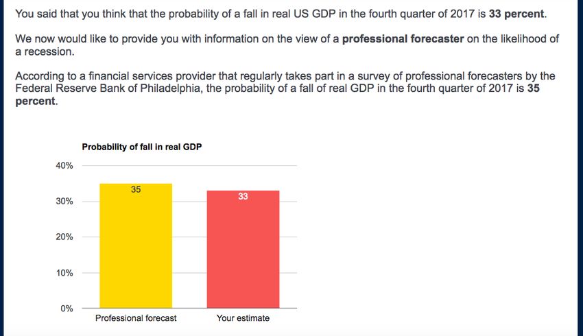
                                                    6

In the “high recession treatment”, respondents receive a forecast from the most pes-
simistic panelist in the SPF, who assigns a 35 percent probability to a fall in US real
GDP in the fourth quarter compared to the third quarter of 2017. In the “low recession
treatment”, respondents receive information from one of the most optimistic forecasters,
who expects a fall in US real GDP with a probability of 5 percent.5 In order to make
the treatment more meaningful to our respondents, we provide them with a figure that
contrasts their prior belief with the prediction from the professional forecaster (see Figure
1 for an illustration of the treatment screen).

Personal expectations, economic behavior, and macroeconomic expectations
After the information provision all respondents are asked to estimate the likelihood that
the unemployment rate in the US will increase over the 12 months after the survey, as well
as a qualitative question on how they expect unemployment to change. This is followed
by questions on personal economic expectations, other macroeconomic expectations and
their consumption plans. While we elicit most expectations probabilistically, we also
include some qualitative questions with categorical answer options.6

    We first ask our respondents whether they think that their family will be better or
worse off 12 months after the survey. Subsequently, we elicit people’s density forecast
about their earnings growth conditional on working at the same place where they cur-
rently work.7 We ask our respondents to assign probabilities to ten brackets of earnings
growth over the next 12 months, which are mutually exclusive and collectively exhaustive.
Respondents could not continue to the next screen if the entered probabilities did not
sum up to 100 percent. The elicitation of a subjective probability distribution allows us
to measure both mean expected earnings growth and uncertainty about earnings growth.8
   5
      The professional forecasts correspond to SPF panelists’ beliefs about a drop in real GDP two quarters
after this wave of the SPF was conducted.
    6
      The question framing we use to elicit people’s expectations closely follows the New York Fed’s
Survey of Consumer Expectations (SCE). The question framing was optimized after extensive testing
(Armantier et al., 2017) and follows the guidelines on the measurement of subjective expectations by
Manski (2017).
    7
      In contrast to the question in the SCE, we also allow for changes in hours worked as well as for job
promotions or demotions at their workplace as this provides us with additional variation.
    8
      Means of density forecasts are easy to interpret, while point forecasts could capture mean, mode or
some other moment of our respondents’ subjective probability distributions (Engelberg et al., 2009).

                                                    7

Thereafter, respondents estimate their subjective probability of job loss and their subjec-
tive probability of finding a new job within three months in case they lose their job over
the next 12 months. In addition, we elicit density forecasts of inflation over the next 12
months using the same methodology as for earnings expectations.9

    Subsequently, we ask our respondents some qualitative questions related to their con-
sumption behavior. First, we ask them whether they think that it is a good time to
buy major durable goods. Second, our respondents are asked how they plan to adjust
their consumption expenditures on food at home, food away from home and leisure ac-
tivities during the four weeks after the survey compared to the four weeks prior to the
survey. Thereafter, our respondents answer a qualitative question on how they expect
firm profits to change over the next 12 months, and they estimate the percent chance that
unemployment in their county of residence will increase over the next 12 months. Finally,
we re-elicit beliefs about the likelihood of a fall in real US GDP in the fourth quarter of
2017 compared to the third quarter of 2017. At the end of the survey, our respondents
complete a series of additional questions on the combined dollar value of their spending
on food at home, food away from home, clothing and leisure activities over the seven days
before the survey, the industry in which they work and their tenure at their employer,
as well as a set of questions measuring their financial literacy.10 Moreover, we ask them
a series of questions on their assets, their political affiliation as well as their zipcode of
residence.

2.3     Follow-up survey

We designed our main survey to minimize concerns about numerical anchoring and ex-
perimenter demand. First, instead of eliciting posterior beliefs about the likelihood of a
recession immediately after the information provision, respondents first answer a range
   9
      We ask our respondents about inflation, as done in the New York Fed’s Survey of Consumer Ex-
pectations, instead of changes in the general price level, as done in the Michigan Survey of Consumers.
Asking consumers to think about prices results in more extreme and disagreeing self-reported inflation
expectations (de Bruin et al., 2011).
   10
      We use the three questions on interest compounding, inflation and risk diversification that have now
become standard to measure financial literacy (Lusardi and Mitchell, 2014).

                                                    8

of other questions and only report posteriors at the end of the survey, roughly 10 minutes
after the information. Second, we elicit both probabilistic and qualitative expectations to
ensure the robustness of our findings to different question framing and numerical anchor-
ing. While we believe that these design features already address some concerns regarding
numerical anchoring, we further mitigate such concerns by conducting a two-week follow-
up survey in which no additional treatment information is provided. We chose to have a
two-week gap between the main study and the follow-up to balance the trade off between
testing for persistence and maximizing statistical power in the follow-up survey.

    In the follow-up survey, we re-elicit some of the key outcome questions from the main
survey, such as the likelihood of an increase in national- and county-level unemployment,
expectations about firm profits, as well as personal economic expectations, such as sub-
jective job security and earnings expectations. We re-elicit our respondents’ estimated
likelihood of a fall in real GDP in the fourth quarter of 2017 compared to the third
quarter of 2017. Moreover, we collect data on our respondents’ consumer and financial
behavior in the time between the main intervention and the follow-up survey. First, we
ask our respondents about their combined spending on food at home, food away from
home, clothing and leisure activities over the seven days before the follow-up survey.11
Second, we ask them whether they bought any major durable goods and whether they ac-
tively increased or reduced their stockholdings during the 14 days prior to the follow-up.
Finally, we elicit our respondents’ beliefs about their employers’ exposure to aggregate
risk, their personal unemployment history, as well as their beliefs about the most likely
causes of a potential recession.

2.4     Discussion of the experimental design

In our experiment we provide respondents with different individual professional forecast-
ers’ assessments of the likelihood of a recession. An alternative experimental design would
  11
     We chose to have a one-week time horizon as this mitigates concerns about measurement error due
to imperfect memory and as we were constrained by the time window between the main survey and the
follow-up. One caveat is that our measure includes categories that are quite lumpy, such as clothing, and
therefore may vary greatly across individuals at the weekly frequency, which could lead to more outliers
and noisier estimates.

                                                   9

provide the average professional forecast to respondents in the treatment group, while giv-
ing no information to individuals in a pure control group. We believe that our design
provides important advantages for studying the causal effect of recession expectations on
personal economic expectations and behavior.

    The variation in recession expectations in the alternative design would stem from
differences between individuals whose beliefs have been shifted, and those who still hold
their prior beliefs. Thus, the alternative design identifies the causal effect of recession
expectations on outcomes of individuals who hold unrealistic priors ex-ante, as the treat-
ment only shifts beliefs for this group. This could threaten the external validity of results
obtained under the alternative design. By contrast, our design also generates variation in
recession expectations among individuals with more realistic priors, and therefore identi-
fies average causal effects of recession expectations for a broader population. In addition,
receiving a forecast may not only shift the level of individuals’ beliefs but may also have
side effects, such as reducing the uncertainty surrounding the level of their beliefs or
priming respondents on recessions and professional forecasts. In our design, the only
difference between the two treatment arms is the percent chance assigned to the event
of a recession by the professional forecast our respondents receive, while side-effects of
receiving a forecast should be common across treatment arms.12

    There are two disadvantages of not having a pure control group. First, a pure control
group would allow us to assess whether the questions and procedures of the experiment
per se induce a change in subjects’ beliefs about a potential upcoming recession. While
this would give an indication of the external validity of our findings, we note that such
changes in expectations should be common across treatment arms and do not threaten
the internal validity of our results. Second, a pure control group would provide us with a
potentially more meaningful benchmark to interpret the magnitudes of the experimentally
estimated causal effects of subjects’ recession expectations on their macroeconomic and
  12
     Moreover, since in the alternative design the treatment intensity is correlated with the level of
the prior belief, heterogeneous effects across groups would conflate differences in priors and differential
extrapolation from macroeconomic to personal expectations. Our design enables a clean analysis of het-
erogeneous extrapolation from aggregate to personal economic expectations across groups, as treatment
intensity is orthogonal to prior beliefs.

                                                    10

personal expectations as well as their behavior.

   Under which conditions will our experimental design generate variation in respon-
dents’ recession expectations? As further discussed in online Appendix D.2 we require
i) that respondents do not fully “de-bias” the signals and thereby perfectly learn about
the average professional forecast and ii) that respondents believe that the professional
forecasts provide a relevant signal about the future state of the economy that is not yet
fully incorporated into their information sets.

2.5       Data

Representativeness Table A2 provides summary statistics for our sample for a large
set of variables. Around 80 percent of our respondents indicate that they are the main
earner in their household. Moreover, Table A3 in the online Appendix13 displays the
distributions of a range of individual characteristics among respondents in full-time em-
ployment in the 2015 American Community Survey (ACS) and in our data. Our sample
matches the distributions of gender, age, region and total household income very pre-
cisely. In addition, the composition of our sample is quite close to the composition of
the population in full-time employment along non-targeted dimensions, such as industry
and hours worked. One caveat is that our sample has higher labor earnings and is more
educated than the US population in full-time employment, similar to the New York Fed
Survey of Consumer Expectations. We address this issue by conducting heterogeneity
analyses according to education and by demonstrating the robustness of our results to
re-weighting (Section 5).

Definition of variables First, we generate a variable measuring the perceive chance of
becoming personally unemployed over the next 12 months as the product of people’s per-
ceived probability of losing their main job within the next 12 months and their perceived
probability of not finding a new job within the following three months. For each respon-
dent we calculate the mean and standard deviation of expected inflation and expected
  13
       The online Appendix is available at https://goo.gl/MTJ8hG.

                                                 11

earnings growth using the mid-points of the bins to which the respondent has assigned
probabilities.14 Moreover, we create an index of people’s planned change in non-durable
consumption from the four weeks prior to the main survey to the four weeks after the
survey, using their qualitative spending plans for food at home, food away from home,
and leisure activities. Finally, we create a measure of people’s actual changes in spending
on food at home, food away from home, clothing and leisure based on their self-reported
spending during the seven days before the main survey and the seven days before the
follow-up survey.15 The questions on expected firm profits, the expected financial situa-
tion of the household and the change in stockholdings between main survey and follow-up
were elicited on five- and seven-point scales. We code these variables such that higher
values refer to “increase” or “improve” and lower values refer to “decrease” or “worsen”.
These qualitative outcome variables are normalized using the mean and standard de-
viation separately for the main survey and the follow-up survey. For the quantitative
measures we do not normalize outcome variables as they have a natural interpretation.

Integrity of the randomization Our sample is well-balanced for a set of key char-
acteristics and pre-treatment beliefs about the likelihood of a recession (Table A5). The
means do not differ significantly across treatment arms for any of these variables and
we cannot reject the Null hypothesis that the partial correlations of the variables with a
dummy for being in the high recession treatment are jointly zero. Moreover, we observe
no differential attrition in our main survey across treatment arms, and participation in
the follow-up survey is not related to treatment status in the main experiment. The
sample of individuals in the follow-up is balanced across the two treatment arms in terms
of key covariates (Table A6). There are marginally significantly more individuals with a
college degree and more men in the low recession treatment arm in the follow-up sample,
but we cannot reject the Null hypothesis that the correlations of the covariates with the
  14
      We elicit probabilities over eight closed bins between -12 percent and 12 percent and two open bins
for outcomes outside this range. For the open bins we assign -14 percent and 14 percent, respectively.
   15
      We take the difference in log spending from the follow-up and the baseline survey, so this variable
measures the percent change in spending. We deal with outliers by setting spending growth to missing
for respondents in the top and bottom two percent of observed spending growth. We obtain qualitatively
similar results if we instead use one or five percent as cutoff, or if we winsorize the variable.

                                                   12

high recession dummy are jointly zero. To rule out any concerns, we include a set of
control variables in all of our estimations.

Data quality We provide evidence that our expectations data on earnings and inflation
are of high quality by comparing our data with a panel survey by the New York Fed that
was launched as a predecessor to the Survey of Consumer Expectations (SCE) (Armantier
et al., 2013). For example, for inflation expectations, 80 percent of our respondents
assign positive probability to more than one bin (89.4 percent in the Fed survey) and the
average number of bins with positive probability is 4.24 (3.83). Although a larger share
of our respondents assign positive probability to non-contiguous bins (6.9 percent vs 0.9
percent), this still accounts for a very small fraction of our sample. Only 0.4 percent,
6.5 percent and 0.3 percent of our respondents enter a prior probability of a fall in real
GDP of 0 percent, 50 percent and 100 percent, respectively, which may indicate mental
overload (de Bruin et al., 2000; Manski, 2017).16

3        Updating of recession expectations

3.1      Prior beliefs

Stylized facts Respondents in our sample have a much more pessimistic macroeco-
nomic outlook than professional forecasters (Figures 2 and A.3 and Table A4). The
median professional forecaster in the second quarter of 2017 reports a likelihood of a
recession in the fourth quarter of 2017 of just 15 percent. By contrast, the median re-
spondent in our sample assigns a probability of 40 percent, as pessimistic as professional
forecasters were for the last time in the second quarter of 2009. While there is a large
dispersion in beliefs about the likelihood of a recession among consumers, the dispersion
of beliefs is much smaller in the sample of professional forecasters, ranging from four
professional forecasters estimating a 5 percent chance of a recession to one forecaster
    16
      Figures A.10 to A.15 display the distributions of future unemployment and inflation expectations,
inflation uncertainty, expected earnings, earnings uncertainty and subjective job loss and job finding
probabilities.

                                                  13

assigning a 35 percent chance.

    We confirm these patterns using robustness experiment 1 (described in more detail
in Table A1), which was conducted with an online convenience sample from the online
labor market Amazon Mechanical Turk (MTurk), which is widely used in experimental
economics research (Bordalo et al., 2016; Cavallo et al., 2017; D’Acunto, 2018a,b; DellaV-
igna and Pope, 2017; Kuziemko et al., 2015; Roth et al., 2019). We discuss the advantages
and disadvantages of MTurk samples in appendix Section C.1. The median professional
forecaster in the second quarter of 2018 reports a likelihood of a recession in the fourth
quarter of 2018 of 10 percent, while the median respondent in our MTurk sample assigns
a probability of 45 percent (Figure A.6). The distribution of recession expectations in
the MTurk sample is remarkably robust to incentivizing the consumers’ forecast using
a quadratic scoring rule (see A.7).17 A Kolmogorov-Smirnov test confirms that the dis-
tributions of incentivized and unincentivized beliefs are not statistically distinguishable
(p=0.319).

    The finding of greater pessimism and a higher dispersion of beliefs among consumers
than those among professional forecasters is in line with previous findings on inflation
expectations (Armantier et al., 2013; Mankiw et al., 2003) and with qualitative expec-
tations on aggregate economic conditions over a longer time period from the Michigan
Survey of Consumers (Das et al., 2018).18

Correlates of recession expectations Neither education nor age are related to peo-
ple’s recession expectations, but females have a significantly more pessimistic macroeco-
nomic outlook than men (Table A7). Interestingly, Democrats are much more pessimistic
compared to Independents, while Republicans are much more optimistic, consistent with
evidence on partisan bias in economic expectations (Mian et al., 2018). People who
have been personally unemployed in the past are significantly more pessimistic about
aggregate economic conditions, in line with Kuchler and Zafar (2018), who find that
  17
      Specifically, respondents in the incentive condition are told that they can earn up to $1 depending
on the accuracy of their forecast.
   18
      In section E.1 in the online Appendix we confirm the external validity of these findings using data
from the New York Fed’s Survey of Consumer Expectations.

                                                   14

individuals who lose their jobs become significantly less optimistic about the aggregate
economy. Taken together, it is reassuring that the correlations between covariates and
recession expectations are in line with previous literature.

3.2    Updating of recession expectations

Do our respondents update their recession expectations upon receiving the professional
forecasts? Figure 2 shows our first main result:

Result 1. The information provision strongly shifts expectations towards the professional
forecast in both treatment arms, and cross-sectional disagreement within the treatment
arms declines. This implies that the respondents were initially not fully informed about
the forecasts and that the forecasts are relevant to the respondents’ economic outlook.

   Figure 3 displays scatter plots of prior and posterior beliefs. Observations along the
red horizontal lines indicate full updating of beliefs towards the professional forecast, while
respondents along the 45 degree line do not update at all. We observe more updating
of beliefs among respondents in the low recession treatment, where the average absolute
distance of prior beliefs to the signal of 5 percent is greater than in the high recession
treatment, which provides a forecast of 35 percent. 11.5 percent of respondents in the
low recession treatment and 19.5 percent of respondents in the high recession treatment
do not update their beliefs at all, while 68.6 percent (47.8 percent) of respondents either
fully or partially update their beliefs towards the signal (see Table A23). The remaining
respondents either “over-extrapolate” from the signal or update in the opposite direction.
However, part of these observed changes in beliefs could be caused by typos or by re-
spondents changing their beliefs because taking a survey on macroeconomic topics makes
them think more carefully about the question. Finally, the cross-sectional disagreement
in posterior beliefs as measured through the interquartile range and standard deviation
declines within both treatment arms compared to prior beliefs (Table A4).

                                              15

Magnitudes We quantify the degree of updating of recession expectations by estimat-
ing a Bayesian learning rule that we derive in online Appendix D.1. We define updatingi
as the difference in people’s posterior and prior expectations, and the “shock” as the dif-
ference between the professional forecast and the prior belief, i.e. (35 - priori ) for people
in the “high recession treatment” and (5 - priori ) for people in the “low recession treat-
ment”. We assume that people’s prior beliefs about the probability of a recession follow
a beta distribution and that the loss function is quadratic. Under these assumptions,
people should follow a linear learning rule, updatingi = α1 shocki , where α1 lies in the
interval [0, 1] and depends negatively on the strength of the respondent’s prior belief.19

    The individual-level shock depends on the respondent’s prior, which introduces two
problems: First, the prior is measured with error, thereby leading to attenuation bias in
the estimated learning rate α1 . Second, self-reported expectations could differ between
the prior and the posterior for reasons that are unrelated to the treatment but potentially
correlated with the prior. Most importantly, people who hold higher priors and are subject
to a more negative shock, should mechanically display more negative changes in their
expectations since the probability of a recession is bounded to be in the interval [0, 100],
leading to an upward bias in the estimate of α1 . Controlling linearly for people’s prior
belief removes attenuation bias and mechanical correlations between people’s updating
and the shock, while not changing the interpretation of the estimated coefficient α1 as
the learning rate. Moreover, we include a vector of additional control variables Xi , which
increases our power to precisely estimate treatment effects and which allows us to control
for the slight imbalance in the follow-up sample.20 Specifically, we estimate the following
equation using OLS:

                       updatingi = α0 + α1 shocki + α2 priori + ΠT Xi + εi                              (1)
   19
      In the case of a beta distribution, confidence in the prior can take the lowest values for individuals
with a prior of 50 percent, but is not mechanically linked to the prior. In a first step we are interested
in the average learning rate over the full sample.
   20
      The controls are as follows: age, age squared, a dummy for females, log income, a dummy for
respondents with at least a bachelor degree, dummies for the respondent’s Census region of residence,
a measure of the respondent’s financial literacy as well as a dummy for Republicans and a dummy for
Democrats.

                                                    16

where εi is an idiosyncratic error term. We report robust standard errors throughout the
paper.

    We estimate a highly significant learning rate equal to about one third of the shock to
individual beliefs (Table 1). Our estimated learning rate from professional forecasts is in
the range of estimates in related literature (Armantier et al., 2016; Coibion et al., 2018a;
Fuster et al., 2018). Thus, our information treatment generates a difference of about 10
percentage points in people’s average posterior beliefs across treatment arms. The size
and significance of the estimated learning rate implies that the respondents found that
the forecasts contain some relevant information that was not already incorporated into
their priors. Online Appendix D.2 provides a more detailed discussion of the estimated
learning rate in the context of different corner cases and estimates in related literature.

Are changes in expectations consistent with Bayesian updating? First, Bayesian
updating predicts that respondents should adjust their expectations partially or fully to-
wards new signals that they find informative, i.e. that learning rates should lie in the
interval [0, 1]. Our estimated learning rate of one third is in line with this prediction.
Second, Bayesian updating implies that respondents who are less confident in their prior
belief should react more strongly to new signals. We examine this prediction by con-
structing a dummy indicating whether the respondent is at least “sure” about his or her
prior estimate. Consistent with Bayesian updating, the estimated learning rate is signifi-
cantly lower for respondents who are more confident in their prior belief (Table 1 column
2). Moreover, respondents who report that they usually do not follow news on the na-
tional economy place significantly higher weight on the signal (column 3), consistent with
the idea that information acquisition prior to the experiment increases the strength of
people’s prior belief.21 In robustness experiment 3 described later we also find support
   21
     We examine whether individuals put differential weight on signals that are more optimistic or more
pessimistic than their prior belief. We interact the individual-specific shock with a dummy variable taking
value one if shock < 0, and zero otherwise. There is no asymmetric updating from relatively positive
and relatively negative signals. Similarly, the weight put on the prior belief does not differ systematically
between the two treatment arms (p=0.443), indicating that our respondents do not differentially weigh
signals that are more or less positive in absolute terms. Finally, we find no significant differences in
learning rates according to the level of people’s prior, confirming that despite the beta distributed priors
confidence is not mechanically linked with the level of the prior. Results on these estimations are available

                                                     17

of two more predictions of Bayesian updating: i) receiving a forecast makes respondents
more confident in their beliefs; ii) changes in confidence are positively related to the
individual-level learning rate (Table A18).

Heterogeneous updating across demographic groups Individuals with lower ed-
ucation update more strongly from the forecasts, while there are no significant differences
according to income, gender, industry, personal unemployment experiences, the unem-
ployment rate in the county of residence and financial literacy (Table A9). Heterogeneity
in learning rates could stem from differences in trust towards experts, differential ex-ante
informedness about the professional forecasts across groups,22 or different learning rules.

    One particular way in which learning rules could differ across individuals is that
less sophisticated individuals could find it more difficult to rationally learn from the
information. As shown in Table A10, the heterogeneity in learning rates according to
confidence in the prior is fully driven by individuals with a college degree, while those
without a college degree weigh the new information independently of their confidence in
their priors. The coefficients on the interaction terms between the shock and confidence
in the prior are significantly different between the two groups (p < 0.01). Thus, while
learning from information is consistent with Bayesian updating for more sophisticated
individuals, less sophisticated individuals seem to follow simpler learning rules. Similarly,
heterogeneity in learning rates by news consumption is fully driven by highly educated
respondents.

Do changes in recession expectations persist? Following Cavallo et al. (2017) we
employ a two-week follow-up survey in which no treatment information is administered.
The medium-run learning rate (calculated using the follow-up) amounts to about 40 per-
cent of the short-run learning rate (Table 1 column 5), in line with respondents receiving
upon request.
   22
      According to theories of rational inattention, individuals with greater exposure to macroeconomic
risk and individuals with lower cost of acquiring information should hold stronger prior beliefs about the
likelihood of a recession. We cannot disentangle these two forces in our data. Note that our analysis
in Section 4.3 examines whether for a given change in expectations about a recession more exposed
respondents extrapolate more strongly to their personal job loss expectations, which enables us to abstract
from differences in information acquisition or trust towards experts across groups.

                                                    18

new relevant signals about the macroeconomy between the two surveys or imperfect mem-
ory (see also Figures 2 and A.4). Moreover, learning rates still differ significantly between
respondents with different confidence in the prior and different levels of news consumption
prior to the survey.

Implications for macroeconomic models Our results presented in this section have
several implications for macroeconomic models. The finding that respondents use the
professional forecasts to persistently update their beliefs implies i) that the professional
forecasts were not fully incorporated into our respondents’ information sets before the sur-
vey and ii) that our respondents consider the information relevant for their expectations
about the future. This finding suggests that there exist costs of information acquisition,
as in micro-founded sticky information models (Reis, 2006).23 Our experiment sets these
costs to zero for a particular piece of news about aggregate economic growth.

    Conditional on acquiring information, we observe heterogeneity in learning rates across
groups. This is in line with the idea that our respondents perceive the piece of information
with individual-specific noise, as in models of noisy information (Maćkowiak and Wieder-
holt, 2015; Sims, 2003). In addition, we also observe heterogeneity in learning rules: On
the one hand, highly educated respondents put lower weight on the information when
they hold stronger priors, in line with the predictions of Bayesian updating. Rational
learning from new information is a key feature of both sticky and noisy information mod-
els, so these models may be able to proxy the expectation formation of more sophisticated
individuals in a reasonable manner. On the other hand, less highly educated respondents’
learning from the information does not seem to be well captured by Bayesian updating,
highlighting a role for cognitive limitations and heterogeneity in belief formation mecha-
nisms in macroeconomic models. These findings are consistent with recent evidence that
individuals with cognitive limitations display larger biases in their expectation formation
(D’Acunto et al., 2019a,b,c). Our findings are inconsistent with more traditional models
  23
     Our evidence on information acquisition costs in the context of news about future economic growth
complements similar findings from experimental studies of information rigidities in households’ expecta-
tions about inflation (Armantier et al., 2016; Cavallo et al., 2017) and house prices (Armona et al., 2018;
Fuster et al., 2018) or firm expectations (Coibion et al., 2018a).

                                                    19

of full-information rational expectations (Muth, 1961) or models with no heterogeneity.24

     Finally, in line with the model and time series evidence in Carroll (2003), our findings
imply that households exhibit some trust towards experts in the context of expectations
about general economic conditions.

4        The causal effect of recession expectations

4.1      Empirical specification

In the previous section we established that our respondents durably update their beliefs
about the likelihood of a recession in response to professional forecasts. This provides us
with a first stage to examine the causal effect of recession expectations on expectations
about personal economic outcomes. Specifically, we examine whether people’s subjective
economic model, as measured through the size and heterogeneity of extrapolation to
expectations about their personal situation, is in line with empirical facts. As a first step,
we examine how these expectations, expi , are correlated with our respondents’ posterior
beliefs about the likelihood of a recession, posteriori :

                               expi = β0 + β1 posteriori + ΠT Xi + εi                                    (2)

where Xi is a vector of the same control variables that we included in our previous estima-
tions. The OLS estimate of β1 cannot be given a causal interpretation. For example, it is
possible that people who are generally more optimistic or pessimistic respond differently
to both the question on the posterior as well as the questions related to the evolution of
other economic outcomes. It is also conceivable that the direction of causality runs from
the personal situation to macroeconomic expectations, as suggested by recent evidence
in Kuchler and Zafar (2018). Finally, the estimate of β1 could be biased towards zero
    24
     Our findings suggest that in a setting where individuals observe one specific piece of information once,
more highly-educated respondents’ learning from information may be well approximated by Bayesian
updating. However, in general, salience could also matter for how much weight individuals put on
information. For instance, D’Acunto et al. (2018b) document that the price changes of more frequently
purchased goods matter more for the formation of inflation and interest rate expectations.

                                                     20

because of measurement error in the posterior belief. To deal with omitted variable bias,
reverse causality and measurement error, we instrument our respondents’ posterior beliefs
with the random assignment to the different professional forecasts, where highrecessioni
is an indicator taking value one for individuals who received the pessimistic professional
forecast, and value zero for respondents receiving the optimistic forecast.. Specifically,
we use two-stage least squares and estimate the following equation:

                                           \ i + ΠT Xi + εi
                          expi = β0 + β1 posterior                                     (3)

where

                         \ i = αˆ0 + αˆ1 highrecessioni + Θ̂T Xi
                       posterior

   We have a strong and highly significant first-stage on people’s post-treatment beliefs
about the likelihood of a recession based on the random assignment of the different
professional forecasts (F-Stat = 75.16; see Table 2).

4.2     Do recession expectations affect personal expectations?

Consistent with the evidence on updating of recession expectations, we establish that the
experimental variation successfully shifts the respondents’ expectations about aggregate
unemployment. Posterior beliefs about a recession significantly affect people’s beliefs
about the probability that the national unemployment rate will increase. In the IV spec-
ification a one percentage point higher likelihood of a recession causes a 0.895 percentage
point increase in the perceived chance that national unemployment will increase (Panel
B of Table 2; column 1). We find similar effects if we use the categorical measure which
is immune to numerical anchoring (column 2). The effect size is 0.536 for the subjective
probability that unemployment in the respondent’s county of residence will increase (col-
umn 3), and slightly lower than for aggregate unemployment. The results on national
and county-level unemployment expectations are significant and of similar magnitude in
the OLS and IV specifications.

   Do recession expectations affect people’s beliefs about their personal economic out-

                                            21

comes? Table 2 shows our second main result:

Result 2. People extrapolate from their recession expectations to their own households’
financial prospects and to expectations about personal unemployment. The estimated effect
sizes are large, but still close to job transitions during the last recession.

People who think that a recession is more probable are also more likely to hold pessimistic
beliefs about their own household’s financial prospects and expect lower earnings growth
in their job. They also report lower levels of subjective job security. The estimated effects
in the IV specifications are very similar in size to the OLS estimates, but the effects on
expected earnings growth become statistically insignificant (Panel B). The effect size on
subjective job security is substantial, yet in line with job losses during the last recession:
a one percentage point increase in the likelihood of a recession leads to an increase in
subjective unemployment risk of 0.113 percent. To illustrate the magnitude of this effect,
consider moving from a situation with zero risk of a recession to a situation in which a
recession will happen with certainty. 11.3 percent of our respondents would then need to
become unemployed for their expectations to be accurate on average. For comparison,
the job loss rate increased by 7 percentage points during the Great Recession 2007-09,
and most laid-off workers remained unemployed for several months (Farber, 2011). Thus,
although the magnitude of our estimated effect is relatively large, it is still close to the
increase in unemployment during the last recession.25

4.3     Heterogeneous extrapolation to personal expectations

Actual differences in risk exposure across groups Actual exposure to macroe-
conomic risk should affect the extent to which people extrapolate from news about the
macroeconomy to their personal expectations. Therefore, we examine changes in un-
employment rates over the Great Recession for different demographic groups using data
   25
      Figure A.16 displays local polynomial regressions of people’s expectations about personal economic
circumstances on their prior beliefs about the likelihood of a recession. The correlations are all strong and
go into the expected directions, indicating that non-experimentally manipulated recession expectations
correlate with personal economic prospects in a meaningful way.

                                                     22