Pork, infrastructure and growth: Evidence from the Italian railway expansion - University of ...
←
→
Page content transcription
If your browser does not render page correctly, please read the page content below
NICEP Working Paper: 2021-04

    Pork, infrastructure and growth: Evidence
       from the Italian railway expansion

                           Roberto Bonfatti
                          Giovanni Facchini
                          Alexander Tarasov
                          Gian Luca Tedeschi
                             Cecilia Testa

Nottingham Interdisciplinary Centre for Economic and Political Research

School of Politics, The University of Nottingham, Law & Social Sciences Building,
University Park, Nottingham, NG7 2RD
ISSN 2397-9771
Pork, Infrastructure and Growth:
       Evidence from the Italian Railway Expansion∗

             Roberto Bonfatti, Giovanni Facchini, Alexander Tarasov,
                           Gian Luca Tedeschi and Cecilia Testa†

                                            July 30, 2021

            This paper studies the role played by politics in shaping the Italian railway network,
       and its impact on long-run growth patterns. Examining a large state-planned railway
       expansion that took place during the second half of the 19th century in a recently
       unified country, we first study how both national and local political processes shaped the
       planned railway construction. Exploiting close elections, we show that a state-funded
       railway line is more likely to be planned for construction where the local representative
       is aligned with the government. Furthermore, the actual path followed by the railways
       was shaped by local pork-barreling, with towns supporting winning candidates more
       likely to see a railway crossing their territory. Finally, we explore the long-run effects of
       the network expansion on economic development. Employing population and economic
       censuses for the entire 20th century, we show that politics at a critical juncture played
       a key role in explaining the long-run evolution of local economies.

       Keywords: Infrastructural Development, Political Economy.
       JEL classification numbers: N01, N73, D72.

   ∗
     We thank Carlo Ciccarelli, Francesco Drago, Peter Egger, Giovanni Federico, Stefano Fenoaltea, David
Nagy, Johanna Rickne, Valeria Rueda, Jim Snyder, Guido Tabellini and seminar participants at the CES-Ifo
Conference on the Global Economy, Royal Economic Society Annual Conference, ETH Zurich, IFW Kiel,
University of Modena and Reggio Emilia and the University of Padua for useful feedback, and Edoardo Cefalá
and Malena Arcidiacono for excellent research assistance.
   †
     Bonfatti: University of Padua and University of Nottingham, roberto.bonfatti@unipd.it; Facchini,
University of Nottingham and CEPR, giovanni.facchini@nottingham.ac.uk; Tarasov, HSE University,
atarasov@hse.ru; Tedeschi: University of Padua, gianluca.tedeschi@unipd.it; Testa: University of Nottingham
and NICEP, cecilia.testa@nottingham.ac.uk.

                                                    1
1. Introduction

There is a widespread belief that a well-designed transport network is at the heart of a
flourishing economy, and indeed transport infrastructure takes up a large share of public
investments around the world. Motivated by these facts, a large literature has attempted to
evaluate the impact of transport infrastructure. One typical approach has been to exploit
some source of quasi-experimental variation in its placement, allowing the researcher to
identify its impact on various economic outcomes. This literature has typically found that
(a) infrastructure has large positive effects on economic activities; (b) the actual process
of allocating infrastructure is not random, suggesting that political factors could play an
important role in the choice of its location (for an overview, see Redding and Turner 2015).
Yet, work on whether and how politics shapes infra-structural development remains scant.
Importantly, since investment in infrastructure has been shown to have both short- and
long-run economic consequences, then if political factors affect investment decisions, short-run
political circumstances may shape long-term local development in a significant way. In this
paper, we make progress on these important questions by analysing the political determinants
of the major railway expansion that occurred in Italy between 1879–1890, and its long-term
effects on economic growth.
    This is an ideal setting for a number of reasons. First, the network expansion set out by
the so-called “Baccarini Law” of 1879 sparkled the second Italian railroad “boom” (Fenoaltea
1983), almost doubling the size of the country’s network in a short period of time.1 Second,
historians have long argued that in the allocation of these lines electoral considerations
played an important role (e.g. see Tajani 1944 and Schram 1997). Finally, weak party
structures in this period implied that personal politics played a crucial role (Larcinese 2021),
providing strong incentives for individual representatives to bring distributive goods to their
constituencies.
    A large literature points out that those in a position of power are able to bring the “bacon”
home (see Larcinese et al. 2013 for an overview). Thus, one key implication of models of
pork-barrel politics is that constituencies represented by elected officials in government are
more likely to be recipients of distributive goods, such as transport infrastructure. Moreover,
if elected government officials reward their partizan supporters, then areas that voted more
for government candidates are more likely to attract investment spending. Importantly, if the
latter affects economic growth, then short run pork-barrel politics may have persistent effects.
In this paper, we bring these predictions to the data to shed light on whether (a) support
   1
     The program had very significant implications for the finances of the new state. Its total cost for the
government was initially estimated at around 1.26 billion Lire, or 12.3% of 1879 GDP, but eventually came
to almost twice that amount (Schram 1997, page 111; Ferrucci 1898; Istat 1957).

                                                     2
for pro-government candidates affects the location of railway infrastructure and (b) political
factors prevailing right after the Italian unification, by shaping infrastructural development,
had long-term effects on economic growth.
In the first part of the paper, following the standard approach in the distributive politics
literature,2 we study how support for pro-government candidates affects the location of
railway infrastructure. We build on a unique dataset combining national election outcomes
at the municipality level and geo-coded historical railway paths. To identify the causal effect
of alignment, we use a regression discontinuity design focusing on close elections, i.e. on
districts in which a pro-government candidate won or lost by a narrow margin.
The railway construction plans on which we focus were laid out in the 1879 Baccarini
Law. The legislation determined the lines to be built by including a list of city-pairs that
would have to be connected, but it did not specify the exact route that each line would have
to follow. We thus proceed in two steps. In the first step, we focus on district-level electoral
outcomes to determine whether municipalities belonging to districts that narrowly elected a
pro-government candidate in 1876 (the election shaping the composition of parliament when
the Baccarini Law was approved) were in closer geographic proximity to a Baccarini Law
line, compared to those narrowly won by a pro-opposition candidate. In the second step, we
focus instead on the actual construction of the railways over the subsequent three legislatures
(1880-82, 82-86, 86-90), and on the exact route that was chosen for them. For this analysis,
we exploit detailed information on voting in approximately 7,000 municipalities. We attain
identification by restricting the sample to municipalities included in marginal districts, and in
close proximity to the Baccarini Law railways. Within this restricted sample, we ask whether
municipalities were more likely to receive a railway depending on the extent to which they
voted for the district’s winning candidate, and whether or not the latter belonged to the
government coalition.
Our results show that pork-barrel politics played an important role both in terms of
which lines were included in the state-planned railway expansion and in determining the path
followed by the railways that were built. In particular, regression discontinuity estimates
comparing municipalities belonging to electoral districts where the government marginally
lost to ones where the government marginally won reveal that Baccarini Law lines are
significantly closer to municipalities in districts carried by the government. Results are robust
to the inclusion of a rich set of municipality-level controls, fixed effects and to varying RD
specifications. Furthermore, studying the actual construction of the planned railways through
the subsequent period reveals that a municipality’s alignment with national politicians played
a very important role: first, municipalities strongly supporting members of parliament elected
2
For a seminal contribution, see Levitt and Snyder (1995).
3in their district are significantly more likely to see a railway crossing their territory; second,
such support is particularly relevant if the elected candidate was affiliated with the government
party.
In the second part of the paper, building on a rich literature studying the contribution of
railways, or more in general transport infrastructure, to economic development, we study
the long-run consequences of the railway expansion promoted by the Baccarini Law. In
particular, we ask whether the impact of politics on the shape of the railway expansion
studied in the first part of the paper had long-lasting consequences on subsequent growth.
To address this question, we digitize detailed municipality-level population and industry data
up to 1991. We deploy a variety of strategies to attain identification. First, we use a rich
set of pre-determined municipality characteristics and demanding fixed effects specifications.
Second, to further improve our comparison of municipalities with similar characteristics and
subject to similar conditions, we focus our analysis on the sample of municipalities that are
in close proximity to the railway lines. Third, we exploit the political conditions that affected
construction of the railways, by further restricting our sample to municipalities belonging
to electoral districts with close races when the construction was contracted out. Fourth,
building on the first part of our analysis, we exploit closeness to instrument for historical
railway access.
Our results show that municipalities that gained railway access thanks to the Baccarini
Law expansion experienced significantly higher population growth in the century following
their construction. This effect was small at the beginning, but it accelerated in the post-WWII
period. A comparison of OLS and IV coefficients reveals that the latter are always smaller than
the former, suggesting that the railways were allocated to disadvantaged towns (that would
have grown less even in the absence of the railways, and that stood to benefit less from the
railways). We also show that population growth was not driven by an increase in employment
in the manufacturing sector, but rather by an expansion in the service industries.3 This
finding suggest that municipalities reached by the Baccarini Law railways became important
hubs providing services to the surrounding areas. Taken together our results represent a
remarkable example of how even minor political events occurring at a “critical juncture”
(Acemoglu and Robinson 2012) may have a big effect on long-run development.
This paper is related to two strands of research. First, it speaks to the literature on
distributive politics and in particular to the comparatively small body of work that has
analysed the allocation of transport infrastructure.4 In an early contribution, Knight (2005)
shows that politicians enjoying positions of power - i.e. members of the US House Committee
3
Margo and Haines (2008) find similar results for the American Midwest in the 19th century.
4
For a recent survey, see Golden and Min (2013).
4on Transportation and Infrastructure – are able to secure more infrastructure funding for
their districts in the 1991-1998 period. Similar patterns were uncovered by Curto–Grau et al.
(2012) for road expenditure across Spanish provinces in the late 19th– early 20th century.
Burgess et al. (2015) study instead the role played by ethnic favoritism on the allocation of
roads in Kenya after independence, finding that districts sharing the same ethnicity as the
president receive twice as much expenditure on roads and have five times the length of paved
roads built. Interestingly, this effect disappears during periods of democracy. Finally, Bogart
(2018) studies how the adoption of river navigation acts by English towns in the late 17th–
early 18th century was affected by political connections. Most of these studies use panel
fixed effect models, whereas we deploy a regression discontinuity design, providing additional
benefits in terms of identification. In addition, relative to this earlier literature, our paper
also explores the long-run implications of pork barrel politics.
Our paper is also related to the recent literature on the impact of infrastructure on growth.
In particular, in an early contribution, Atack et al. (2010) show that railway access had a large
positive impact on urbanization in the American Midwest in the 1850-1860. Hornung (2015)
and Büchel and Kyburz (2020) document a positive effect of railway access on city population
growth rates in 19th century Prussia and Switzerland respectively. Taking a longer time
perspective, Berger and Enflo (2017) document a similar effect in Sweden over a 150 years
period. Most of these papers deploy an IV methodology based on the inconsequential units
approach (Banerjee et al. 2020) – using straight line or least cost paths corridors between
two main nodes – typically uncovering a downward bias in the OLS estimates. As Hornung
(2015) points out, the bias might be due to an omitted variable, as “... cities with lower
growth prospects might have influenced routing in order to become connected”(page 714). In
our paper, using quasi–random variation in assignment to treatment due to political factors,
besides showing that secondary railroads in Italy were indeed allocated to disadvantaged
towns, we provide evidence on the political channel through which towns gained influence in
shaping the railroad paths.5
The paper is organized as follows. Section 2 provides a historical overview of railway
expansion and elections in Italy in this period. Section 3 describes the data. Section 4
discusses the results linking electoral outcomes and railway development. Section 5 discusses
the results analysing the long-run consequences of railway access on economic development.
Finally, Section 6 concludes.
5
While these papers estimate the relative impact of the access to the railroad, other studies have considered
general equilibrium approaches. See for example Donaldson and Hornbeck (2016) and Donaldson (2018).
52. Historical Background
In this section, we provide background information on the development of railroads in Italy
in this period, and on the evolution of the Italian electoral system.
2.1. Railway constructions in Italy, 1876-1913
In this paper, we focus on the railway expansion overseen by the governments of the “Historical
Left” (1876-1896), which dealt mainly with the realization of the secondary lines required
to connect smaller towns and cities to the main lines built by the “Historical Right” in the
previous decade. Demand for these type of infrastructure had been strong since the 1860s,
as the unconnected towns and cities complained that the main lines drew economic activity
away from them (Maggi 2003, p. 63). However, construction only began with the advent of
the Left and responded to this political group’s need to consolidate its power base (see e.g.
Tajani 1944 and Mercurio 1994). The key legislative milestone was the so-called “Baccarini
Law” of 1879 which set out the plan of railway expansion for the next two decades.6 This was
a controversial initiative – the transcripts of the parliamentary debates around this act exceed
1,500 pages – and over 600 amendments were proposed and defended in many speeches, one
of them lasting two days. Crucially, as Schram (1997) points out (p. 111) “Clearly,... the
members of parliament could not resist the temptation to advance their electoral interests by
promoting the construction of a railway line in their own constituency.” Based on this plan,
6,794 km of new lines were added between 1879 and 1913, of which 96% were contracted out
for construction before 1890 (Table 1), and 89% were completed before 1896, when the Left
was ousted from power (Appendix Table A.1).
The construction of the Baccarini Law railways was a major financial undertaking by the
national and local governments. The law set aside a large sum to be spent by the national
government on the new railways (1,260 million Lire, or 12.3% of 1879 GDP; see Istat 1957),
and the actual cost of the network realization turned out to be significantly larger (Ferrucci
1898; Tajani 1944). At the same time, the law dictated that part of the costs of construction
should be shouldered by the interested provinces and municipalities, as further explained
below. The constructions were initially slowed down by financial troubles, for two main
reasons. On the one hand, many provinces and municipalities proved unable to contribute to
the costs of construction. On the other hand, the cost estimates on which the initial funding
assignments relied proved too low, based as they were on very rough technical studies. In
many cases, actual construction costs turned out to be more than twice as high as initially
6
We exclude from our sample a few lines which were built in this period, despite being approved by earlier
laws.
6Figure 1. Railways Expansion in Italy, Pre- and Post-1879
Railway expansion under Baccarini Law (1879-1913)
Pre-1879 railways
Notes: Extent of the Italian railway network before 1879 and lines constructed between 1879 and 1913 under
the Baccarini Law. Authors’ elaborations based on the data by Ciccarelli and Groote (2017).
expected (Tajani 1944, pp. 94-95). As a result, only 1,491 km of new lines were completed by
1886, or about 22% of the total (see Appendix Table A.1). To speed up the constructions, the
government passed new laws in 1885-1888, setting aside additional funding and increasing the
role of the private sector.7 This led to an acceleration in the constructions between 1886-1890.
However by the early 1890s, the Italian State was in serious financial troubles, to the point
that it could not afford to run the 1891 census. Many blamed the railways for this situation
(Ferrucci 1898, p. 7).
In this paper, we study whether the railway constructions of this period were shaped
7
The State outsourced 1,000 km of railway constructions (amongst which some of those in our sample) to
the three private companies which operated the Italian railways from 1885 onwards.
7by electoral competition. As already hinted above, it has long been argued that they were.
To understand the political context, it is important to note that Italy did not have a well-
structured party organization in the late 1870s. Rather, the political scene was dominated by
two loose coalitions of factions, the Historical Right and the Historical Left. Representatives
had very little loyalty to a particular group, and Trasformismo – defined by Collier (1999) as a
“...system of political clientelism based on the formation of ad hoc parliamentary groups that
monopolized political office by using patronage and fraudulent elections to ensure electoral
success” – was rampant. As a result, individual members of parliament, free from party
discipline, were particularly forceful in advancing the interests of their constituencies. Not
surprisingly, given the vast amount of public funding involved in the railway investment
program, the latter came to the forefront of Italian politics in the late 1870s and 1880s.
As reported by the Corriere della Sera (the main national newspaper), “... the House of
Representatives has turned into a large railway electoral academy.”8 Members of parliament
often centered their campaigns on the promise to bring railways to their constituency (Maggi
2003, p. 67), and contemporary commentators accused the ruling majority of using the
railways to help the political and economic fortunes of its own people (Tajani 1944, p. 94-95).9
To investigate this empirically, we exploit a peculiar feature of the Baccarini Law. The
law grouped the railways into five categories, in decreasing order of national importance and
financial contribution by the State.10 There was an important distinction between category
1-3 lines, on the one hand, and category 4-5 lines on the other. In the former case, the
Baccarini Law determined exactly which lines should be built, by providing lists of city pairs
that should serve as start and end points. The law, however, did not describe the exact route
to be followed.11 There were 4,490 km of category 1-3 lines. As for category 4-5 lines, the
law merely authorized the government to construct up to 2,530 km of category 4 lines, and
to allow the construction of an unspecified amount of category 5 lines.12 Appendix Figure
8
“La Camera si é trasformata in una grande accademia ferroviaria elettorale” in Tutti Gabbati, May
25-26 1879.
9
Perhaps not surprisingly, Fenoaltea (1983) finds that many of the lines built in this period generated
little operating revenues. According to Fenoaltea, the Left’s lines did decrease transport costs more than
main, North-South lines constructed by the Right: while facilitating defence, the latter were largely unable to
compete with sea transport.
10
The construction of category 1 lines was entirely financed by the State, while category 2-4 lines only
attracted a 90%-60% state contribution (the rest being shouldered by the affected provinces and municipalities).
Category 5 lines, to which here we add 581 km of Sardinian lines approved by a 1885 law, were entirely
financed by the relevant provinces or municipalities, or by private companies. Profits from operating category
2-4 lines would be shared between the State and the other investors according to their initial contributions,
while profits from category 5 lines would be entirely appropriated by non-State investors.
11
For example, the law would say that a category 1 line connecting the cities of Faenza and Pontassieve
should be built, a category 2 line connecting the cities of Bassano and Primolano, and so on. The lists
remained essentially unaltered in the following two decades.
12
The limit for category 4 lines includes an additional 1,000 km that were added by a 1885 law. Maggi
8A.3 draws the two groups of railways in two separate maps.13
This feature of the law naturally suggests a two-step empirical approach. There are two
distinct stages at which politics may have affected the allocation of category 1-3 lines, the
ones on which we focus in this paper. The first stage was the shaping of the Baccarini Law
itself. As explained above, the Law provided lists of city pairs that should serve as start and
end point of a new line. The politics of the 1876-1879 period may have shaped decisions on
which city pairs to include in these lists. We study whether this was the case, by analysing
whether electoral districts that were aligned with the government in the 1876 election were
more likely to be crossed by a least cost path connecting some of the city pairs listed in the
Baccarini Law (full details on identification and the construction of the least cost paths are
provided in later sections).
The second stage in which politics may have mattered was the construction stage. The
Baccarini Law did not specify the exact route to be followed by the new lines, or the order
of construction. Thus, before a line connecting cities A and D could be built, a feasibility
study would have to identify the technical challenges to be overcome, and the exact route
to be followed between A and D (e.g. passing through city B as opposed to city C); the
State bureaucracy would have to approve this study; and finally, the government would have
to contract out the construction of the line. The latter stage was typically done by trunks:
in the example above, the A-B trunk could be contracted out at a different date than the
B-D trunk. Presumably, this procedure left some leeway for the post-1879 governments to
influence the exact routes that would emerge from the feasibility studies produced under
their remit. Thus, for each trunk contracted out after 1879, our hypothesis is that political
factors at play in the legislature in which the trunk was contracted out may have shaped
both the decision to contract it out, and its exact location.
We test for this hypothesis by using variation at the municipality level. In particular,
we ask whether municipalities located in a corridor around a least cost path connecting
some of the Baccarini Law city pairs were more likely to receive a railway during a post-
1879 legislature, if they had aligned with the government at the start of that legislature.
By “receiving a railway”, we mean that the construction of a trunk cutting through the
municipality’s territory was contracted out during the legislature under consideration. Table 1
reports the cumulative km of lines contracted out during each post-1879 legislature. The focus
(2003), p. 65, argues that demand for category 4 lines largely exceeded supply. According to this author, this
category was introduced in order to give members of parliament, whose district would not be connected by
category-1-3 lines, the hope (but no firm commitment) that they could still be connected by a category 4 line.
The government’s assumption was that, without such a provision, the law would never have passed.
13
All category 1-3 lines would be built “by the State” (though the actual constructions was contracted
out to private companies), while the construction of category 4-5 lines could be outsourced to the relevant
provinces or municipalities, or to the private sector.
9Table 1. Km. of railways contracted out and completed, as compared to
predicted by Baccarini Law (1879)
1st − 3rd 4th 5th
Total
category category category
Km. contracted out during legislature:
1876 - 1880 275 0 0 275
1880 - 1882 1,041 531 94 1,666
1882 - 1886 1,166 538 180 1,885
1886 - 1890 1,604 207 882 2,693
Total (1876-1890) 4,086 1,276 1156 6,519
Total km. completed (1876-1913): 4,360 1,276 1,156 6,794
Total km. predicted by Baccarini Law: 4,490 2,530 - 6,620
Notes: The 2530 km of predicted category-4 lines include the 1000 km added to this category by
the Legge 27 aprile 1885 n. 3048. Authors’ elaborations based on the data by Ciccarelli and
Groote (2017).
of our analysis will be on the three legislature spanning the period between 1880 and 1890.
We disregard the 1876-80 legislature since very few lines were contracted out in this period.
We also disregard the post-1890 legislatures, for two reasons. First, the near-bankruptcy
of the Italian State meant that the official publications on which we rely become much
more patchy after 1890, calling into question the reliability of the data. Second, as already
mentioned, 96% of the Baccarini Law lines were contracted out for construction before 1890.
In summary, we will be studying how election results in the 1876, 1880, 1882 and 1886
elections determined, first, the choice made in 1879 on which city pairs to connect, and
second, the choices on the exact routes that these railways should follows, which we assume
were made shortly before the lines were contracted out for construction in 1880-1890. To
better understand the politics of this period, we now turn to reviewing the existing electoral
rules.
2.2. Electoral systems
The Italian Constitution during the Kingdom of Italy envisioned a bicameral system, with
a House or Representatives elected by the population and a Senate whose members were
appointed for life by the King. The two chambers had similar powers, and legislation
10had to clear both in order to be enacted by the King. Our focus will be on the House of
Representatives, whose electoral system evolved quite significantly across the four elections
we consider (1876, 1880, 1882 and 1886), in terms of both electoral rules and the extent of
the franchise. In the 1876 and 1880 elections, representatives were chosen according to a
standard majoritarian rule, with single-member electoral districts and runoff voting. There
were 508 districts and in each of them the candidate who obtained the most votes was elected,
as long as he had been supported by at least one third of the eligible voters, and one half of
the votes cast (excluding invalid votes). If no candidate satisfied these requirements, then
the two candidates with the most votes proceeded to a second round, in which the winner
was selected by simple majority. Second rounds were frequent under this electoral rule: they
occurred, on average, in 30% of the electoral districts in the 1876 and 1880 elections.
In 1882, a major reform introduced a majoritarian rule with multi-member districts and
runoff voting. Districts became fewer and larger: there were 135 of them, electing a number
of representatives varying between 2 and 5.14 In each n-seat electoral district, voters could
cast n preferences (at most one per each candidate), with the exception of 5-seat districts
where voters could only cast 4 preferences.15 The n candidates with the most votes were
elected, provided they had obtained at least as many votes as one eighth of the eligible voters.
Where some seats had remained unfilled, the unelected candidates with the most votes (in
a number equal to twice the number of seats to be filled) proceeded to a second and final
round. There were very few second rounds under this rule: they occurred in only 2% of the
electoral districts in the 1882 and 1886 elections.
The extent of the franchise was very low throughout the period, but increased significantly
with the reform of 1882. Both before and after the reform, only males could vote. Before the
reform, the franchise was strictly based on income: only individuals older than 25 years and
declaring an annual income of at least 40 Lire were allowed to vote (with a few exceptions
made for high-skills professions). As a result, only about 2% of the population was allowed
to vote in 1876 and 1880. The 1882 reform reduced the age requirement to 21 years and
the income requirement to 19.8 Lire, and abolished the income requirement for individuals
holding the mandatory elementary school degree (2 years of schooling), as well as for an
extended number of high-skills professions. As a result, the franchise rose to more than 7%
of the population (see Appendix Table A.2).
14
The law specified the number of seats to be attributed to each province. Such number was proportional
to the province’s population, and was to be updated in the first parliamentary session after the publication of
each population census. The law went on to subdivide provinces into electoral districts, in a number varying
between 1 and 5.
15
The rationale for 5-seat districts was to make it easier for important minority group to elect at least one
representative (see the discussion in Brunialti 1882, pp. 250 onwards).
113. Data
We assembled a novel dataset covering approximately 7,000 Italian municipalities, including
data on railway development, electoral outcomes and a wealth of socio-economic characteristics
observed at various points in time between 1863 and 1991. One issue that we face is that
municipalities did not remain identically defined over this period. For example, some of
them merged to form larger municipalities, others split to form smaller ones, some acquired
territory from others, and there were denomination changes and transfer of municipalities
across larger administrative units (e.g. provinces, regions).
To address this issue, we used information from Sistema Informativo Storico delle Am-
ministrazioni Territoriali (SISTAT) to adjust the territories of the municipalities to be at
constant 1991 borders.16 SISTAT is a database maintained by the Italian National Institute
of Statistics (ISTAT) reporting any territorial or administrative changes that municipalities
have gone through since 1861. Its data allows us to keep track of denomination changes, and
any territorial changes involving municipalities as a whole. The most frequent case is mergers,
e.g. municipalities A and B merging to form municipality C at time t < 1991. In this case,
when collecting historical data for time t1 < t, we separately collected data for A and B,
and then aggregated up so that only C appears in our dataset at time t1 . In a much smaller
number of instances, municipalities split, e.g. C splitting into A and B at time t < 1991.17
In this case, for any t1 < t for which we have access to data, we first collect the observation
referring to C, and we then use population weights in 1991 to split this observation into A
and B, so that these municipalities also exist in our dataset in t1 < t. This procedure does
not allow us to track territorial changes at the level below the municipality. For example,
if municipality A incorporated 10% of the former territory of municipality B, then we can
not take care of this, since our minimal unit of observation is the municipality. This kind of
changes in territory were minor and infrequent, however.
3.1. Railways and Elections
Our analysis focuses on the railway expansion plan laid out by Baccarini Law of 1879. The
vast majority of these railways were contracted out for construction in 1880-1890, and opened
by 1895 (see Table 1 and Appendix Table A.1). Our starting point is the database by
16
For consistency, we use constant 1991 borders also for provinces, another administrative unit considered
in the analysis.
17
Municipalities were mostly aggregated during this period, as evidenced by the fact that there were 8,400
municipalities in 1871, but only 7,700 in 1991, at constant 1871 national territory. The decades immediately
after World War II were exceptional in this respect, since many mergers that had occurred during the Fascist
era were reversed afterwards. For this period, we only use population data which was independently adjusted
to be at constant 1991 municipal boundaries by Sistema Statistico Nazionale (1994).
12Ciccarelli and Groote (2017), which is based on historical sources and maps and provides a
georeferenced reconstruction of the development of the Italian railway network spanning the
period 1839-1913. In this GIS dataset, the authors digitise railway segments as line features,
and provide additional information such as year of opening, main/secondary line classification
and a distinction between standard and narrow gauges. Since our municipalities are defined
at constant 1991 boundaries, we combined this database with the 1991 shapefile of Italian
municipalities, which is also the earliest provided by ISTAT.18 This procedure allowed us to
determine the list of municipalities that each new railway trunk cut through.
We begin by constructing measures of the stock of railways (if any at all) present on each
municipality’s territory in 1876, the date of the first election in our sample. Next, we identify
the Baccarini Law lines in our GIS dataset, and proceed to determine the date in which
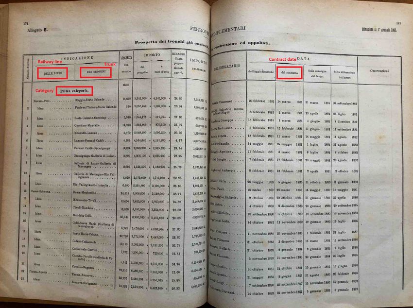
the construction of each trunk was started. To this end, we have located detailed reports
summarizing information on procurement contracts, at the trunk level, reporting the contract
award date (see Ministero dei Lavori Pubblici (1885), Ministero dei Lavori Pubblici (1889)
and Ministero dei Lavori Pubblici (1891)).19 Appendix Figure A.4 presents an example of
the information available in the reports we have used.
Next, we have matched the contract award date with the corresponding legislature and
the elections that determined its composition. Data on parliamentary election outcomes
have been obtained from Corbetta and Piretti (2009). This source provides digitised data on
Italian parliamentary elections from 1861 to modern times, at the district and municipality
level. Our elections of interest are 1876, 1880, 1882 and 1886.
The district-level data contains the name of the district, the number of registered voters,
the number of voters who cast a ballot and the name and political affiliation of the elected
candidate(s). For the 1876 and 1880 elections, in which representatives were chosen in
single-member districts, we also have information on the number of votes obtained in the
district by the winning candidate. For the 1882 and 1886 elections, in which a variable number
of representatives (between 2 and 5) were elected in districts at large, we have information
on the number of preferences obtained by each elected candidate. Since Corbetta and Piretti
(2009) do not provide data on the number of votes or preferences obtained by the losing
candidates in the district, we obtained this information digitising data from Nuvoloni (1898).
These sources allowed us to collect the same information for run-off elections, which took
place on average in 30% of the districts in the 1876 and 1880 elections, and in 2% of the
districts in the 1882 and 1886 elections. Appendix Table A.2 provides summary statistics on
18
We exclude from the analysis the North-Eastern parts of the country that were only annexed after World
War I
19
We decided not to use the completion date by Ciccarelli and Groote (2017) for this purpose, since
completion could lag the start of construction by up to several years.
13district-level population, franchise and turnout in the four elections in our sample.
Corbetta and Piretti (2009) also provide municipality-level electoral outcomes.20 For the
1876 and 1880 elections, for all municipalities located in a district, they report the votes
obtained by all candidates in the district. This gives us the total number of votes cast in the
municipality, and hence the share of votes obtained by candidates who were elected in the
district as well as those who were not. For the 1882 and 1886 elections, the municipality-level
data of Corbetta and Piretti (2009) only reports the number of preferences obtained by
the candidates who were elected in the district. To complement this data, we collect and
digitize information on registered voters and number of voters who cast a ballot at the
municipality level for the 1882 and 1886 elections from original archival sources, e.g. the
Archivio della Camera Regia. Based on the number of voters who cast a ballot and the
number of allowed preferences in the district to which the municipality belongs, we estimate
the share of preferences obtained in the municipality by each elected candidate.21
3.2. Additional socio-economic characteristics
The existing literature has highlighted the role played by a number of additional socio–
economic factors in determining whether a locality is connected by a railroad. To account for
them, we assemble a rich set of municipality-level characteristics from a variety of historical
sources.
We obtain population figures spanning the period 1861–1991 by digitizing data from
Sistema Statistico Nazionale (1994).22 Importantly, these data refer to municipalities bound-
aries as defined in 1991 and thus matches the information we have on the presence of
railroads and political outcomes. We additionally employ this population data to construct a
municipality-level measure of market access.23
We have then digitized information on other indicators of initial economic development, e.g.
the presence of a post office, telegraph office, railway station or sea port in 1871 (from Ministero
20
More precisely, the electoral outcomes for municipalities reported by Corbetta and Piretti (2009) are
based on data at the level of sezione, an electoral division whose relation to the municipality depended on
the latter’s size and on the extent of the franchise. For small municipalities in the early part of our sample a
“sezione” would often encompass multiple municipalities, in which case we assign to each of municipality the
electoral result of the “sezione” they belong to.
21
Specifically, we compute the share of preferences obtained by each elected candidate as the ratio between
the number of preferences cast in favor of the candidate in the municipality and the number of total number
of voters who cast a ballot in the municipality multiplied by the number of allowed preferences.
22
Censuses were held every ten years except for 1891 and 1941, when they were not held, and 1936, when
an additional census was held.
23
We follow the standard approach in Pthe literature to obtain our measure of market access, where for
−1
each municipality i we compute M Ai = i6=j Pj Dij , with P being the population of municipality j, and D
the geodesic distance between municipalities i and j. In the calculation of M Ai we employ the population of
all municipalities, with the exception of municipality i’s own population.
14dell’Interno 1874), and the number of secondary schools and libraries of municipalities in 1863
(from Ministero dell’Educazione Nazionale 1866 and Ministero dell’Educazione Nazionale
1865). For our long-run analysis we have also collected information on a series of additional
municipality-level characteristics, which have been digitized from a series of inquiries carried
out in the 1880s. In particular, we obtained data on hygienic and sanitary conditions in
1885 from Direzione Generale della Statistica (1886), covering quality and quantity of water
available, percentage of roads with sewage system, percentage of houses with toilets, number of
doctors, number of pharmacies, number of hospital beds and number of years with registered
cases of cholera. We supplement this information digitizing data on public revenues and
expenditures in 1884 from Ministero di Agricoltura, Industria e Commercio (1887), including
total municipal revenues as well as revenues from real estate and land taxes and expenditures
on public education, to capture local investment in human capital acquisition.
We additionally collected information on a series of time-invariant geographic characteris-
tics. Using the FAO-GAEZ database, we have constructed ten separate municipality-level
indexes on suitability for growing agricultural crops.24 To account for the role played by
difficult terrains, particularly in obstructing railway passage, we used data on terrain rugged-
ness from Nunn and Puga (2012) to construct a municipality-level Terrain Ruggedness Index
(TRI). Finally, we compute measures of land area, elevation and an indicator for municipalities
situated on the sea coast.
Table 2 and Appendix Table A.3 provide summary statistics on the various municipality-
level characteristics we collected.
4. Elections and Railway Constructions
In this section, we study the role of electoral competition in shaping the development of the
Baccarini Law lines. We start by analysing the decision to include a line in the law, and then
turn to explain the actual route followed in its construction.
4.1. Identification
The decision to build the railroads considered in our analysis can be articulated in two
steps. The first involves the choice of including a railway line in the Baccarini Law of 1879.
As already mentioned, the law specified the initial and end (focal) points of each line, but
no additional detail was provided on the route to be followed. The second step involves
instead the choice of the path of the various trunks which were subsequently built, and whose
24
In particular, we have information on barley, bean, cereals, citrus, cotton, oat, olive, rice, rye and wheat
– with suitability varying between 0 (lowest) and 1 (highest).
15Table 2. Summary Statistics on Municipality-Level Characteristics
Mean S.D. Min Max
Pre-1879 and geographic characteristics
Log population density in 1871 4.5751 0.8106 0.6530 9.9889
Post office in 1871 0.3551 0.4786 0 1
Telegraph office in 1871 0.1491 0.3562 0 1
Railway station in 1871 0.0922 0.2893 0 1
Sea port in 1871 0.0059 0.0765 0 1
Number of secondary schools and libraries in 1863 0.1030 0.6234 0 22
Market access 0.3757 0.1326 0 1
Wheat suitability 0.3594 0.2081 0 1
Cereals suitability 0.2943 0.2528 0 1
Rice suitability 0.0707 0.1805 0 1
Cotton suitability 0.1755 0.2162 0 1
Barley suitability 0.3634 0.2089 0 1
Rye suitability 0.3713 0.1989 0 1
Olive suitability 0.3047 0.1899 0 1
Citrus suitability 0.1751 0.2521 0 1
Oat suitability 0.3605 0.2089 0 1
Bean suitability 0.3397 0.1926 0 1
Terrain ruggedness 0.1823 0.1799 0 1
Log land area 3.0807 1.0064 -2.1295 6.3868
Elevation (m) 429 422 0 2,699
Coast 0.0806 0.2723 0 1
Additional characteristics (post-1879)
Quantity of water 2.6924 0.5960 1 3
Quality of water 2.7811 0.7765 1 4
% of roads with sewage 0.1292 0.2693 0 1
% of houses with toilets 0.4452 0.2952 0 1
Number of farmacies (per capita) 0.0003 0.0004 0 0.0045
Number of medics (per capita) 0.0005 0.0005 0 0.0112
Number of years with colera epidemics 1.4847 1.5089 0 11
Number of hospital beds (per capita) 0.0008 0.0063 0 0.4491
Revenue tax on terrains (log per capita) 1.4675 0.5017 0 4.0726
Revenue tax on buildings (log per capita) 0.4847 0.2911 0 1.9581
Municipal surtax (log per capita) 1.4492 0.6224 0 4.1623
Total tax revenues (log per capita) 2.2397 0.4235 0.4686 5.2679
Education ordinary expenses (log per capita) 0.7649 0.2013 0 3.0933
Education extraordinary expenses (log per capita) 0.0903 0.3189 0 4.0723
Education optional expenses (log per capita) 0.1161 0.2074 0 2.4050
Notes: Authors’ elaborations. Data sources described in Section 3.
construction was contracted out between 1880-1890. We are interested in understanding the
role of politics in shaping both these decisions. In particular, if representatives in the ruling
majority are in a better position to reward their constituency with public investments, then
constituencies aligned with the government are more likely to receive railway infrastructure.
16The key identification challenge in our context is that, according to models of distributive
politics, electoral outcomes are endogenous with respect to the allocation of transport
infrastructure.25 We address this concern by deploying a regression discontinuity design
focusing on close races, where the choice of one candidate over another can be thought of
as being as good as random. In other words, our analysis uses randomized variation which
derives from the candidates’ inability to precisely control the assignment variable (e.g. which
candidate wins the election) near the 50% cutoff (Lee and Lemieux 2010).
This assumption would be violated if candidates were able to manipulate the margin
of victory, with a resulting discontinuity at the 50% vote share cutoff. We rule out the
presence of sorting around the threshold by implementing a McCrary test (McCrary, 2008)
(see Appendix Figure A.5) showing the absence of discontinuities around the 50% vote share
threshold. Another concern could be omitted variable bias: the observed empirical correlation
between alignment and railway allocation could be driven by socio-economic determinants
influencing both outcomes. To verify that our RD design addresses this issue, we study
whether all other relevant features aside from the treatment do not systematically differ
at the 50% vote share threshold, e.g. that observations just below the threshold serve as
an appropriate counterfactual for those just above it. In particular, we examine whether
socio-economic and geographic characteristics are balanced across electoral districts that were
marginally won or lost by government party candidates. Our results in Appendix Table A.5,
indicate that there are no systematic differences in the covariates around the 50% vote share
threshold.
While implementing our RD design one, an important caveat applies. As pointed out in
Section 2, while in the 1876 and 1880 elections representatives were chosen in single member
districts (SMD), by 1882 a new electoral law prescribed the creation of districts at large (AL),
in which a variable number of representatives (between 2 and 5) were elected. In the SMD
system, the definition of a close race is based on the gap between the vote shares received by
the winner and the runner up, whereas in the AL system, we focus on the (normalized) gap
in the vote share received by the last of the elected candidates and the first of the non-elected
ones.26
In the first step of the process, representatives elected to the 1876-80 legislature compete
for inclusion in the Baccarini Law of 1879 of a railway line cutting through their electoral
districts. If alignment matters, we expect those supporting the existing government to be in
25
For example Voigtlaender and Voth (2014) show that the construction of the German Autobahn network
in the 1930’s was crucial to consolidate the Nazi party’s grip on power.
26
In particular, let Wd be the vote share received by the least popular of the elected candidates, and let
Ld be the vote share received by the most popular of the non–elected candidates. The normalized gap is then
d −Ld
given by W Wd +Ld .
17a better position to exert influence. To assess whether this is the case, we focus on electoral
outcomes at the district level and implement a sharp regression discontinuity design where
we compare districts in which the government candidate marginally won to those in which he
marginally lost. More formally, we estimate the following specification:
ymd = β0 + β1 GovW ind + f (M argind ) + β2 Xmd + σp + emd (1)
where m denotes the municipality and d the electoral district.
The dependent variable, ymd , captures the proximity of the municipality to the railways
planned for construction by the Baccarini Law of 1879. We measure this in two alternative
ways. First, we consider the log of the distance in km of the municipality’s centroid from the
nearest planned railway. Second, we define two indicator variables, taking a value of one if
the municipality falls respectively within a distance of 10 km or 5 km from a planned railway.
We map a planned railway as the least cost path connecting the focal points of the line as
specified on the Baccarini Law, which we simulate based on the cost estimates related to
distance, slope and river crossings (See Appendix Figure A.1 for an illustration of how the
least cost paths are constructed).27
The regressor of interest is GovW ind . It is an indicator taking a value of one, if the
government carried the district in the 1876 election, and zero otherwise. The term f (M argind )
is the RD polynomial, which allows us to flexibly control for the impact of the distance
between the share of the government party and the 50 percent threshold. Finally, σp is a
vector of province fixed effects and Xmd is a vector of pre–determined municipality level
characteristics, including log population density, presence of post office, telegraph, port,
railways or railway station on the territory, total number of secondary schools and libraries,
market access, terrain ruggedness, agricultural suitability, log land area, elevation and location
on the coast. Our coefficient of interest is β1 , capturing the effect of a government’s party
victory at the discontinuity point (i.e. the 50 percent threshold) on the relevant outcome
variable.
Turning now to the actual realization of the railroads, our hypothesis is that once a
line has been authorized by the Baccarini Law, different municipalities compete to shape
the actual path that will be followed. We thus focus on municipalities located in close
proximity to the planned railway lines (i.e. at a distance of either 10 km or 5 km from
the least cost paths connecting start to end) and consider the role played by local – i.e.
27
We experimented with alternative ways to specify the least cost paths, namely: varying the cost
parameters associated with slopes and river crossings; employing “per-capita construction costs” weighting
cost parameters by population; and using simple straight lines connecting the focal points of the planned
railways. All these different specifications provide similar simulated corridors and comparable estimation
results.
18municipality level – political outcomes. We posit that municipalities, more strongly supporting
candidates that end up winning the district, are in a better position to see railroad lines
constructed on their territory. To identify this effect, we focus once again on close races, i.e.
on districts in which the elected candidate won by a small margin. Under the assumption
that municipality electoral outcomes – on average – do not systematically affect district-level
ones, the assignment of municipalities to treatment is as good as random and thus we can
causally estimate the effect of siding with the winner on receiving a railway project. We thus
estimate the following model:
Railmdj = γ0 + γ1 W inSharemdj + γ2 Xmd + σp + emdj (2)
where Railmdj is an indicator variable taking a value of one if a railroad whose construction
was contracted out during legislature j crosses the territory of the municipality m in district
d and zero otherwise; W inSharemdj is the share of votes received in the municipality by the
candidate who carried the district in that legislature and σp and Xmd denote once again
province fixed effects and pre–determined municipality level characteristics.28 Our coefficient
of interest is γ1 and captures the effect of greater support in the municipality for the marginal
winner of the election compared to the marginal loser.
4.2. Constituency representation and Baccarini Law lines
The first step of our analysis consists in determining whether the inclusion of a railway line in
the Baccarini Law of 1879 was driven by the lobbying of members of parliament on behalf of
their own constituents. In particular, we focus on district-level electoral outcomes for the 1876
election, which determined the composition of the parliament that passed the aforementioned
law in 1879.
Our estimates are based on equation (1), where we regress a series of municipality-level
outcomes – capturing the geographic proximity to railways planned by the Baccarini Law –
on an indicator for whether the government carried the district to which the municipality
belongs. Through this part of the analysis, we adopt a sharp regression discontinuity
design where we study our outcomes of interest at the 50% vote share threshold, comparing
municipalities belonging to district where the government party marginally lost to those
where the government party marginally won.29 To account for potential correlation in the
28
In a robustness check reported in Appendix Tables A.17 and A.18 we also deploy a richer set of controls,
with the caveat that the relevant information is available only for the 1880s, i.e. after the enactment of
the Baccarini Law. These additional socio-economic measures, capturing hygienic and sanitary conditions,
and the amount of public revenues and expenditures, allow us to more precisely account for the municipal
development level when the the railway construction plans were implemented.
29
Marginality is defined using the election round in which the winner is selected.
19estimated relationship across nearby municipalities, we employ spatially-adjusted standard
errors, following the methodology of Conley (1999), based on a window of 20 km around the
municipality’s centroid.
Table 3 reports the results from the RD estimates. In odd-numbered columns, we employ
the full sample of almost 7,000 municipalities across 458 electoral districts.30 These estimates
include a third-order RD polynomial on the distance of the government party vote share
from the 50% threshold, fitted separately on each side of the threshold.31
Table 3. Baccarini Law’s Railway Projects and 1876 District-Level Elections:
Regression Discontinuity Estimates
(1) (2) (3) (4) (5) (6)
Dependent variable: log(km) dist. from projects 10 km proximity to projects 5 km proximity to projects
RD polynomial order: 3rd 2nd 3rd 2nd 3rd 2nd
Margin: - ± 5% - ± 5% - ± 5%
Government-party win in district -0.3578*** -0.3594** 0.1977** 0.2690** 0.2206*** 0.3581***
(0.1263) (0.1804) (0.0797) (0.1199) (0.0694) (0.0972)
Adjusted R2 0.517 0.746 0.262 0.531 0.204 0.465
Observations 6,957 1,471 6,957 1,471 6,957 1,471
Number of electoral district 458 102 458 102 458 102
Municipality-level controls X X X X X X
Province FE X X X X X X
Notes: The table reports reports RD estimates. The unit of observation is a municipality. The dependent variable is the distance
in log(km) from the railway projects in columns (1)-(2); a binary indicator for being in a 10 km proximity to the railway projects
in columns (3)-(4); a binary indicator for being in a 5 km proximity to the railway projects in columns (5)-(6). The distance and
proximity measures are based on least cost paths connecting the focal points indicated by the Baccarini Law. The explanatory
variable indicates a government-party win in the electoral district, with 3rd-order polynomials on the margin of victory being
employed in odd-numbered columns and 2nd order polynomials in even-numbered columns. In even-numbered columns, the
sample is limited to electoral districts where the government-party candidate’s vote share was within a 5% distance of the 50%
threshold needed for election. Municipality-level controls include: log population density in 1871, presence of post office, telegraph,
port, railway or railway station on the territory in 1871, total number of secondary schools and libraries in 1863, market access,
terrain ruggedness, agricultural suitability, log land area, elevation and presence of a coast. All specifications employ province
fixed effects. Standard errors adjusted for spatial correlation, based on a 20 km window, in parenthesis. ***, **, and * indicate
statistical significance at the 1%, 5% and 10% levels, respectively.
Across all three dependent variables, the estimates present a clear discontinuity at the
50% threshold. In particular, column (1) shows a negative discontinuity in the distance of
the municipality from the planned railways (represented as a least cost path connecting the
destination points indicated on the Baccarini Law) in districts secured by the government
party. Similarly, columns (3) and (5) show a positive discontinuity in the likelihood of a
30
Our sample does not include 50 districts representing very large municipalities incorporating multiple
electoral districts because in this case the electoral district is smaller than our unit of analysis, e.g. the
municipality. Furthermore, these very large municipalities were already reached by the main railway network
by 1879.
31
While in Table 3 we only show the coefficient on the main explanatory variable for reasons of space, in
Appendix Table A.4 we also report the coefficients on the control variables.
20You can also read