Probabilistic Mapping and Spatial Pattern Analysis of Grazing Lawns in Southern African Savannahs Using WorldView-3 Imagery and Machine Learning ...
←
→
Page content transcription
If your browser does not render page correctly, please read the page content below
remote sensing
Article
Probabilistic Mapping and Spatial Pattern Analysis of
Grazing Lawns in Southern African Savannahs Using
WorldView-3 Imagery and Machine
Learning Techniques
Kwame T. Awuah 1, * , Paul Aplin 1 , Christopher G. Marston 2 , Ian Powell 3
and Izak P. J. Smit 4,5
 1   Department of Geography and Geology, Edge Hill University, St. Helens Road, Ormskirk L39 4QP, UK;
     Paul.Aplin@edgehill.ac.uk
 2   Land Use Group, UK Centre for Ecology and Hydrology, Library Ave, Bailrigg, Lancaster LA1 4AP, UK;
     cmarston@ceh.ac.uk
 3   Department of Biology, Edge Hill University, St. Helens Road, Ormskirk L39 4QP, UK;
     powelli@edgehill.ac.uk
 4   Scientific Services, Kruger National Park, Private Bag X402, Skukuza 1350, South Africa;
     izak.smit@sanparks.org
 5   Centre for African Ecology, School of Animal, Plant and Environmental Sciences, University of the
     Witwatersrand, Private Bag 3, Johannesburg 2050, South Africa
 *   Correspondence: awuahk@edgehill.ac.uk

 Received: 22 September 2020; Accepted: 11 October 2020; Published: 15 October 2020

 Abstract: Savannah grazing lawns are a key food resource for large herbivores such as blue
 wildebeest (Connochaetes taurinus), hippopotamus (Hippopotamus amphibius) and white rhino
 (Ceratotherium simum), and impact herbivore densities, movement and recruitment rates. They also
 exert a strong influence on fire behaviour including frequency, intensity and spread. Thus, variation
 in grazing lawn cover can have a profound impact on broader savannah ecosystem dynamics.
 However, knowledge of their present cover and distribution is limited. Importantly, we lack a
 robust, broad-scale approach for detecting and monitoring grazing lawns, which is critical to
 enhancing understanding of the ecology of these vital grassland systems. We selected two sites in
 the Lower Sabie and Satara regions of Kruger National Park, South Africa with mesic and semiarid
 conditions, respectively. Using spectral and texture features derived from WorldView-3 imagery,
 we (i) parameterised and assessed the quality of Random Forest (RF), Support Vector Machines (SVM),
 Classification and Regression Trees (CART) and Multilayer Perceptron (MLP) models for general
 discrimination of plant functional types (PFTs) within a sub-area of the Lower Sabie landscape, and (ii)
 compared model performance for probabilistic mapping of grazing lawns in the broader Lower Sabie
 and Satara landscapes. Further, we used spatial metrics to analyse spatial patterns in grazing lawn
 distribution in both landscapes along a gradient of distance from waterbodies. All machine learning
 models achieved high F-scores (F1) and overall accuracy (OA) scores in general savannah PFTs
 classification, with RF (F1 = 95.73 ± 0.004%, OA = 94.16 ± 0.004%), SVM (F1 = 95.64 ± 0.002%,
 OA = 94.02 ± 0.002% ) and MLP (F1 = 95.71 ± 0.003%, OA = 94.27 ± 0.003% ) forming a cluster
 of the better performing models and marginally outperforming CART (F1 = 92.74 ± 0.006%,
 OA = 90.93 ± 0.003%). Grazing lawn detection accuracy followed a similar trend within the Lower
 Sabie landscape, with RF, SVM, MLP and CART achieving F-scores of 0.89, 0.93, 0.94 and 0.81,
 respectively. Transferring models to the Satara landscape however resulted in relatively lower
 but high grazing lawn detection accuracies across models (RF = 0.87, SVM = 0.88, MLP = 0.85
 and CART = 0.75). Results from spatial pattern analysis revealed a relatively higher proportion of
 grazing lawn cover under semiarid savannah conditions (Satara) compared to the mesic savannah
 landscape (Lower Sabie). Additionally, the results show strong negative correlation between grazing

Remote Sens. 2020, 12, 3357; doi:10.3390/rs12203357                     www.mdpi.com/journal/remotesensing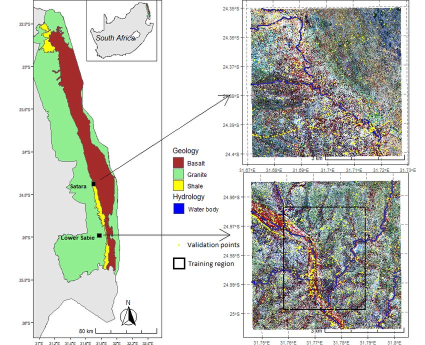
Remote Sens. 2020, 12, 3357                                                                         2 of 37

 lawn spatial structure (fractional cover, patch size and connectivity) and distance from waterbodies,
 with larger and contiguous grazing lawn patches occurring in close proximity to waterbodies in both
 landscapes. The proposed machine learning approach provides a novel and robust workflow for
 accurate and consistent landscape-scale monitoring of grazing lawns, while our findings and research
 outputs provide timely information critical for understanding habitat heterogeneity in southern
 African savannahs.

 Keywords: African savannah; grazing lawns; machine learning; WorldView-3; Support Vector
 Machines; Random Forest; Multilayer Perceptron; decision trees; spatial analysis

1. Introduction
      Savannah ecosystems inherently exhibit a considerable degree of variability in structural and
physical attributes across their range of occurrence [1]. In Southern Africa, they feature the coexistence
of grasses and an overstorey layer of trees with varying gradients of dominance and spatial
formations [2]. Within the grassy layer, plant forms are typified structurally by tall bunch grasses and
short grass grazing lawns [3], which form a significant component of the heterogeneity in Southern
African savannah grasslands [4].
      The relative proportions and distribution of grazing lawns and tall bunch grass resources have
been directly linked to important ecosystem changes such as fluctuations in herbivore density [5,6] and
changing fire regimes [7,8]. For example, the amount of high-quality lawn grasses has been suggested
to be the primary natural limiting factor to population size of mega-herbivores such as the white
rhinoceros (Ceratotherium simum) and the hippopotamus (Hippopotamus amphibius) [6,7,9]. Additionally,
the persistence of grazing lawns creates natural barriers to the spread of fire due to limited above
ground fuel biomass that may serve as fuel for the spread of fire [7,10,11]. By contrast, tall bunch
grasses keep their moribund growth forms and increase savannah grassland fuel load [7,12]. As such,
changes in grazing lawn coverage and distribution could potentially alter the size, frequency and
intensity of fire within the landscape [7], with cascading effects for nutrient cycling, plant community
composition, habitat structure and biodiversity. Monitoring the occurrence and spatial patterns of
grazing lawns is therefore fundamental to understanding the ecology of these vital grassland systems.
      Grazing lawns are dynamic and maintained by constant grazing, resulting in a feedback of dense
nutrient-rich plant growth that in turn attracts more grazing [10]. Different parts of a landscape
may also be predisposed to grazing lawn formation due to localised availability of resources and
nutrient hotspots that concentrate grazers. These include areas around water bodies and areas of
mineral accumulation (e.g., sodium) [10]. The initiation of a cycle of regular grazing thus appears to
be a critical factor for their development and persistence [10–12]. Nonetheless, the rates and specific
pathways of their development likely depend on factors such as rainfall, fire and soil types [13].
Rainfall has a strong influence on the rate of grass biomass accumulation and the height of tall grass
stands [14]. The relative proportion of grazing lawns to high biomass tall grasses is also influenced
by dynamics in soil nutrients through their strong influence on grass productivity. Under high
rainfall and soil nutrient conditions, increased grazing frequency is required to prevent the invasion
of tall-grass competitors [10]. Too infrequent grazing increases the vulnerability of a switch to tall
bunch grasses [11]. Fire also consumes grass biomass and has the potential to shift grass community
composition and structure within different environmental constraints [15]. Tall bunch grasses with
low forage quality dominate fire-driven grassy systems [10–12]. Additionally, post-fire regrowth can
also attract grazers away from previously established grazing lawns causing them to be invaded by
tall bunch grasses [11,12]. The varying spatial and temporal nature of the key interacting factors that
drive grazing lawn dynamics urges for a robust landscape-scale approach to better understand their
variation over space and time.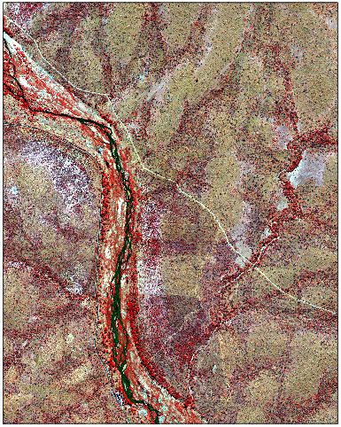
Remote Sens. 2020, 12, 3357                                                                          3 of 37

      Ground-based monitoring of grazing lawn responses to the complex top-down and bottom-up
ecological processes is challenging due to the large areas involved. Although ground-based methods
can provide more detailed and valuable local insights [16], they are not efficient in capturing
regional-scale dynamics—due to the high cost involved—nor do they provide any retrospective
information beyond the start of monitoring activities [17]. Remote sensing technology is able to
overcome the spatial and temporal limitations, which in combination with ground-based observations,
offers valuable tools for accurate, efficient and cost-effective ways for vegetation monitoring [18,19].
      Medium resolution satellite imagery such as the Landsat Operational Land Imager (OLI) [20]
and Sentinel-2 missions [21] are freely available, with extensive temporal coverage which offers
enormous benefits for monitoring vegetation dynamics. Further, recent advances in very high
spatial resolution (VHR) satellite imagery such as WorldView-3 presents opportunities to partially
overcome limitations in spatial resolution associated with medium resolution imagery, particularly in
heterogeneous savannah landscapes [17]. At nadir spatial resolution of 1.24 m [22], the WorldView-3
sensor is able to identify and discriminate between different sized vegetation components such as
trees, shrubs and grass patches [17,23]. Additionally, the yellow, red-edge and two near-infrared bands
in WorldView-3 imagery provide the capability of reliably detecting photosynthetically active or dying
plants and foliar chlorophyll content [24]. As such, various phenological stages of vegetation can be
monitored, which is instrumental in dealing with spectral similarity of different savannah vegetation
composition [23,25].
      In parallel with advances in remote sensing imaging technology, free open source software
packages and increased computational power have been developed to facilitate image analysis.
The combination of these factors has advanced the use of machine learning algorithms in land cover
classification [26]. Among the most popular machine learning classification algorithms are Random
Forest (RF) [27], Support Vector Machines (SVM) [28], Decision Trees (DT) [29] and Artificial Neural
Network (ANN) [30]. RF, SVM, DT and ANN are nonparametric classifiers and are very efficient in
dealing with nonlinear classification problems [26,31], having been proven to be effective in different
savannah ecosystems. Camargo et al. [31] demonstrated the utility of RF, SVM, DT and ANN in
classifying land cover in the Brazilian Tropical Savannah biome. RF is well known for its flexibility
of application on both continuous and categorical datasets, either as a regression or classification
algorithm, respectively [26,27]. Symeonakis et al. [32] used RF to classify different land cover types in
southern African savannahs and reported a maximum accuracy of 91.1 %. The SVM classifier is popular
for its strong ability to generalise in complex nonlinear feature space [28]. SVM was used in seasonal
separation of vegetation components in southern African savannahs and gave the highest accuracy
score under dry leaf-off conditions compared to k-Nearest Neighbour (k-NN), Maximum Likelihood
Classifier (MLC), RF and DT classifiers [23]. The application of DT in an eastern African savannah
resulted in an increased mapping accuracy over MLC and SVM, with over 93% overall accuracy [33].
ANN classifiers have been widely used in satellite image classification, due to the capability to adapt
and generalise different input data structures [26]. The successful application of ANN has been
well demonstrated in different remote sensing contexts, including classification of endangered tree
species [34] and dynamic modelling of land cover changes in semi-arid landscapes [35].
      Much of the literature on monitoring grazing lawn dynamics in southern African savannahs
focuses on localised and controlled experimental studies of responses to the mechanisms that induce
their establishment and persistence [4,10–12]. There is limited evidence on whether the proposed
pathways translate into broad-scale spatial patterns in grazing lawn occurrence. Among the few
empirical studies is the work of Archibald et al. [12] who mapped grass structural distribution and
found that the extent of grazing lawns was directly related to fire return interval. Though there is
substantial information on how different biotic and abiotic factors shape grazing lawns, knowledge of
their present cover and distribution, which is critical to understanding habitat heterogeneity, is lacking.
More importantly, there is no robust, broad-scale approach for detecting and monitoring grazing lawns
to enable comprehensive investigation into their dynamics over space and time, and the implications
Remote Sens. 2020, 12, 3357                                                                          4 of 37

for broader ecosystem dynamics. Against this backdrop, we seek to develop a robust machine learning
framework for mapping grazing lawns in southern African savannahs by (i) parameterising and
assessing the quality of Random Forest (RF), Support VectorMachines (SVM), Multilayer Perceptron
(MLP) and Classification and Regression Trees (CART) models for savannah land cover classification
in a localised context, and (ii) comparing model performance for probabilistic mapping of grazing
lawns on a wider scale. Additionally, we analyse spatial patterns in grazing lawn distribution along
a gradient of proximity to water bodies, which has been hypothesised to influence grassland spatial
structure [10,36].

2. Materials and Methods

2.1. Study Area
      Kruger National Park (KNP) lies between 30◦ 530 18”E, 22◦ 190 40”S and 32◦ 010 59”E, 25◦ 310 44”S
in South Africa. The park spans approximately 20,000 km2 , extending about 360 km from north
to south. The significant diversity in the landscape is expressed in its climate, soil, flora and
fauna, making it a globally important site for ecological studies. The climate is subtropical with
maximum mean annual rainfall between 500 mm and 700 mm in the northern and southern parts
of the park, respectively [37]. Geologically, KNP is divided into granitic soils to the west and
basaltic soils to the east, which are separated by a narrow band of shale from the south to the
mid portion of the park and rhyolite on the eastern extreme [38]. This, coupled with spatial and
temporal rainfall gradients, as well as disturbance events, exert enormous influence on vegetation
type distribution across the landscape [6]. More open, productive grasslands occur on the basalt, while
denser bushland savannah occupy the granite. Mopane (Colophospermum mopane), red bushwillow
(Combretum apiculatum) and silver clusterleaf (Terminalia sericea) constitute some of the dominant
vegetation types in the northern half of the park [37]. The open grasslands of the eastern plain
are dominated by species like blue buffalo grass (Cenchrus ciliaris), red grass (Themeda triandra),
stinking grass (Bothriochloa radicans) and finger grass (Digitaria eriantha), dotted with knob-thorn acacia
(Acacia nigrescens) and marula trees (Sclerocarya birrea) [39]. Mixed broadleaf woodlands of bushwillow
(Combretum sp) with corridors of grassland cover the central-western part of KNP, while thorn thickets
(e.g., Acacia robusta), silver clusterleaf (Terminalia sericea) and sour grasses (Hyparrhenia filipendula)
form a dominant part of the higher rainfall southern landscape [39]. Alongside variations in abiotic
factors which influences vegetation type distribution within the KNP landscape, the presence of a great
diversity of herbivores exert significant impact on vegetation structure. For example, high population
density of the African elephant (Loxodonta africana) has been suggested to be the major driver of woody
vegetation change in KNP [17,40]. The dominant grass consumers (with >50% of grass in diet) includes
impala (Aepyceros melampus), blue wildebeest (Connochaetes taurinus), zebra (Equus quagga), buffalo
(Syncerus caffer) and white rhino (Ceratotherium simum) [41].
      Management of KNP is generally focused on maintaining habitat heterogeneity through adaptive
fire management regimes [38] alongside natural fire events. Natural burns vary in frequency
and intensity depending on rainfall patterns and the prevalence of high grass biomass [37,42].
The consequence of varying fire regimes is the different spatial configurations of grass productivity
and biomass accumulation [42]. For example, the distribution of short grass grazing lawns whose
persistence depends on positive feedback loops associated with frequent grazing has been observed to
be highly influenced by variation in burn size and frequency [11,12].
      Two study sites located within the Satara and the Lower Sabie regions of the park (Figure 1), each
covering 5.7 × 5.7 km, and extending over a range of habitat conditions including rainfall, geology
and vegetation type were used. The Satara site is a well-studied grazing system close to the latitudinal
center of KNP, and covers both granitic and basaltic soil types interspersed with a strip of ecca shales.
The landscape is semiarid with mean annual rainfall of 400–500 mm. The granite areas to the west
are generally more wooded and undulating than the flat and more open and grassy basaltic plains.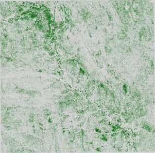
Remote Sens. 2020, 12, 3357 5 of 37
In contrast, the Lower Sabie site falls under mesic landscape conditions with mean annual rainfall
of 600–700 mm. The area has an underlying granite geology and encompasses portions of the Sabie
River catchment. A number of sodic sites are also present within the Lower Sabie study site. Sodic
sites typically occur at footslopes of catenas and are known to have high soil and vegetation sodium
content which concentrates grazers and aids the formation and maintenance of continuous grazing
lawn patches [10].
Figure 1. Map of study area showing locations of the Satara and Lower Sabie field sites in Kruger
National Park (KNP), with enlarged views of the WorldView-3 satellite scenes (False colour: NIR1, R,
G) overlaid with hydrology. Inset map shows the location of KNP within South Africa. Geological
information was obtained from South African National Parks data repository
2.2. Land Cover and Classification Scheme
The study sites were selected to exclude as much anthropogenic influence as possible due to
the natural ecological focus of our study. Thus, natural and semi-natural land cover features such
as vegetation patches, bare soil surfaces and waterbodies dominate the selected study sites, with the
only artificial surfaces being roads and isolated structures which serve as rest stops and picnic sites for
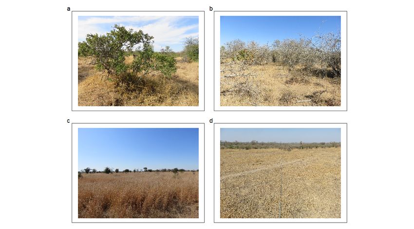
tourists. Four plant functional types (PFTs) were identified in order to distinguish grazing lawns from
other vegetation types (Figure 2). These included evergreen woody components, deciduous woody
components, bunch grasses and short grass grazing lawns.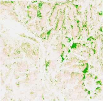
Remote Sens. 2020, 12, 3357                                                                        6 of 37

      Figure 2. Examples of Plant Functional Types (PFTs): (a) woody evergreen, (b) woody deciduous,
      (c) bunch grass and (d) grazing lawns.

      The PFT categories were finalised following the vegetation nomenclature provided in [17] and
were modified based on knowledge from dry season field survey and the spectral reflectance properties
of the different vegetation components contained within satellite imagery. Within the landscape,
woody components are mainly trees and shrubs, which in many cases were challenging to objectively
differentiate. This is a well-known dilemma in savannah landscapes due to structural complexities such
as multiple stems, varying disturbance adaptations and height limitations [43]. The common practice
has been to use arbitrary morphological traits like diameter and height thresholds depending on
research objectives and ecological relevance. For example, [17] used a main trunk diameter threshold
of 7 cm to distinguish between trees and shrubs, where woody components with >7 cm diameter were
classified as trees and those with 20 cm. In contrast, grazing lawns were identified as short grass areas
with stoloniferous growth forms and height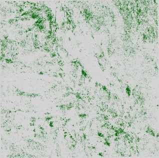
Remote Sens. 2020, 12, 3357                                                                             7 of 37

and 1.85◦ off Nadir) for the Lower Sabie and Satara sites, respectively, under cloud-free conditions.
Dry season imagery has previously been used to successfully discriminate vegetation types in similar
contexts [17,44]. Apart from the reduced persistence of cloudy conditions in the dry season, which is an
advantage to optical satellite remote sensing particularly in the tropics [32], spectral differentiation is
maximized due to phenological differences among different vegetation types [17,45]. Image acquisition
was timed to coincide with our field survey season (June 26–July 21, 2019), which allowed for the
collection of consistent reference information for land cover classification and validation.

      Figure 3. Sample display of land cover types from WorldView-3 satellite image scene (False colour:
      NIR1, R, G). (a) Woody evergreen; (b) Woody deciduous; (c) Bunch grass; (d) Grazing lawn; (e) Water
      body; (f) Bare; (g) Built-up; (h) Shadow.

2.3.2. Reference Data
     Reference data on the different land cover types were generated from georeferenced field survey
locations, and were extended via further interpretation of VHR images augmented by field photos
and Google Earth satellite scenes. Overall, data from (i) 111 predefined field locations, systematically
distributed within 200 m buffer beyond 100 m distance from access roads, and (ii) 5122 randomly
distributed points from augmented visual interpretation, formed the reference data points (i.e., total of
5233 points) for training (3807—i.e., 73%—reference points) and validation (1426—i.e., 27%—reference
points). Polygons of spectrally homogeneous areas were manually digitised and labelled according to
land cover class IDs (see Table 1) using the locations of training points. The polygon extents (Table 1)
were then used to extract image pixels for model training. Of the many potential approaches that
could be used to extract training pixels, polygon objects have been shown to provide the most accurate
classification outcomes [46,47]. Spectral plots of the different land cover classes were examined and
reviewed alongside Jefferies–Matusita distance measures to ascertain adequate spectral separability
prior to model training [48]. Models were parametrised and trained for prediction based on data
from a sub-area within the Lower Sabie field site (see training region in Figure 1). This was necessary
to ensure high model quality as a greater proportion of the georeferenced field sample locations
was concentrated within the training region, while reducing computational cost. In contrast, map
validation was conducted using site-specific reference data.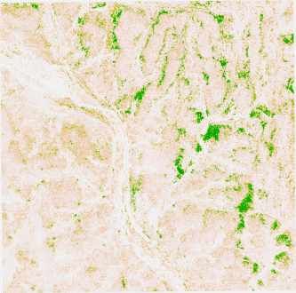
Remote Sens. 2020, 12, 3357                                                                                                                                                               8 of 37

      Table 1. Description of land cover classification nomenclature and reference data. Numbers represent number of reference points, while figures in parenthesis
      represent area of training polygons in hectares. Lower Sabie and Satara validation points are separated by “/” (i.e., Lower Sabie/Satara).

                                                                        Land Cover                                                                                  Reference Samples
ID    Name                    Description                                                                                                                    Model Training   Map Validation
                              Woody vegetation components that are adapted to retain their leaves all year round. Classified based on dry
1     Woody evergreen                                                                                                                                        863 (3.94)       100 / 80
                              season field observations.
                              Woody vegetation components that are adapted to retain their leaves in the wet season and shed them in the
2     Woody deciduous                                                                                                                                        1047 (3.26)      100 / 65
                              dry season. Classified based on dry season field observations.
3     Bunch grass             Tall grass patches with height >20 cm, and often occur as dense patches with upright growth form.                              680 (10.12)      100 / 114
4     Grazing lawn            Short grass patches with height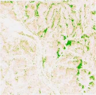
Remote Sens. 2020, 12, 3357                                                                              9 of 37

2.3.3. Auxiliary Data
      Multiple buffer distances (100 m divisions) from water source were used to analyse spatial pattern
in grazing lawn distribution. Water points represent significant resources and important predictors of
grazer movement [49] and spatial heterogeneity in general within semi-arid savannah landscapes [50].
The data (Table 2) was downloaded from OpenStreetMaps surface water archive (streams, rivers and
reservoirs) [51] and was validated against a drainage network and stream order data obtained from
the Scientific services of South African National Parks. The OSM surface water layer contributed in
November 2019 had the closest temporal coverage to the acquisition dates of satellite imagery and
field data, and was selected for spatial analysis.

2.4. Preparation of Image Features
      Following acquisition, a cubic convolution resampling approach was used to upsample images to
2 m spatial resolution, which is reflective of the average minimum patch size of short grass grazing
lawns in southern African savannahs [6,7]. We calculated a series of spectral indices highlighting
greenness, moisture and soil properties in order to increase utility of the spectral information contained
in the original image bands (Table 3). Greenness, moisture and soil indices are derived from arithmetic
combination of spectral information recorded in visible and near-infrared image bands and exhibit
high correlation with vegetation characteristics such as phenology [52–54], biomass [55–57] and
moisture content [58,59]. To complement the spectral information, spatial heterogeneity measures
were calculated as a selection of simple and advanced Haralick texture features based on Gray Level
Co-occurrence Matrix (GLCM) [60]. The GLCM variables (Table 3) were calculated on the near-infrared
band (NIR1) (see Table 2 for details on image bands), which contains valuable spectral information for
differentiating vegetation characteristics. We used a probabilistic quantizer, with 32 quantization levels
in a 3 × 3 moving window, at an offset distance of 1 pixel in all directions (0◦ , 35◦ , 90◦ and 135◦ ) [32,61].
In total, 27 spectral indices and 18 texture features were processed using the Orfeo-Toolbox remote
sensing image processing software [62] (Table 3). The spectral indices as well as texture features in
combination with the original image bands served as input data in the machine learning models and
analysis workflow (summarised in Figure 4). Incorporating spectral and textural image features is
well known to enhance discrimination space for more accurate land cover mapping particularly in
heterogeneous savannah landscapes [32,63,64].

      Figure 4. Conceptual workflow showing steps in machine learning model development and evaluation
      towards grazing lawn detection.
Remote Sens. 2020, 12, 3357                                                                                                                                                      10 of 37

                                                         Table 3. Initial image features serving as potential predictors.

Data (abbreviation)                                                                                    Description
Spectral features from individual bands (B):
                                                                                                       Coastal, Blue, Green, Yellow, Red, Red Edge, Near Infrared-1, Near Infrared-2
B_C, B_B, B_G, B_Y, B_R, B_RE, B_NIR1, B_NIR2
                                                                                                       Normalized Difference Vegetation Index, Transformed Normalized Vegetation
                                                                                                       Index, Ratio Vegetation Index, Soil Adjusted Vegetation Index, Transformed
                                                                                                       Soil Adjusted Vegetation Index, Modified Soil Adjusted Vegetation Index,
Spectral features from vegetation (V), moisture (M) and soil (S) indices:                              Modified Soil Adjusted Vegetation Index-2, Global Environment Monitoring
V_NDVI, V_TNDVI, V_RVI, V_SAVI, V_TSAVI, V_MSAVI, V_MSAVI2, V_GEMI, V_IPVI, V_LAI,                     Index, Infrared Percentage Vegetation Index, Leaf Area Index, Normalized
M_NDWI, M_NDWI2, M_MNDWI, S_BI2, S_BI, S_CI, S_RI, S_NDSI, S_SI1, S_SI2, S_SI3, S_SI4, S_SI5, S_SI6,   Difference Water Index, Normalized Difference Water Index-2, Modified
S_SI7, S_SI8, S_SI9                                                                                    Normalized Difference Water Index, Brightness Index-2, Brightness Index,
                                                                                                       Color Index, Redness Index [62], Normalized Difference Salinity Index, Salinity
                                                                                                       Index-1, Salinity Index-2, Salinity Index-3, Salinity Index-4, Salinity Index-5,
                                                                                                       Salinity Index-6, Salinity Index-7, Salinity Index-8, Salinity Index-9 [65]
                                                                                                       Energy, Entropy, Correlation, Inverse Distance Moment,Inertia, Cluster shade,
Haralick texture features (T):
                                                                                                       Cluster prominence, Haralick correlation, Mean, Variance, Dissimilarity,
T_Ener, T_Ent, T_Corr, T_IDM, T_Iner, T_CS, T_CP, T_HCorr, T_Mean, T_Var, T_Diss, T_SAvrg, T_SVar,
                                                                                                       Sum average, Sum variance, Sum entropy, Difference of Entropies,
T_SEnt, T_Dent, T_DVar, T_IC1, T_IC2
                                                                                                       Difference of variances, Information correlation-1, Information correlation-2 [62]
Remote Sens. 2020, 12, 3357 11 of 37
2.5. Feature Selection
Remote sensing image features such as spectral indices (vegetation, moisture and soil indices) as
well as texture variables tend to exhibit high levels of collinearity. Highly correlated features increases
data redundancy and risk of overfitting, which could have adverse consequences for algorithm
performance especially for high-dimensional datasets [66], a problem that results from the Hughes
phenomenon [67]. Although nonparametric machine learning algorithms are thought to be less
susceptible to Hughes phenomenon, recent findings shows they benefit from dimensionality reduction
nonetheless [68]. In our case, we aimed to target the most robust predictor set while reducing
prohibitive computational efforts.
Image variables were selected by combining two procedures. First, we checked for collinearity
with the Variance Inflation Factor (VIF) using the “usdm” package [69] within R-programming
environment [70]. This was done separately for the spectral indices (i.e., vegetation, moisture and soil)
and the Haralick texture features derived from the WorldView-3 imagery (see Table 3). VIF measures
the degree to which predictor variables are correlated. For example, given k independent predictor
variables, each variable is regressed with the remaining k − 1 variables and coefficient of determination
(R2 ) is estimated. The VIF of the dependent variable is thus computed as
1
V IF = (1)
1 − R2
Large values of VIF implies a corresponding high degree of collinearity and vice versa. Following
VIF analysis, correlated variables were subsequently removed by considering a stepwise elimination
threshold of VIF ≥ 10 [71]. The VIF assessment resulted in six spectral indices and 15 Haralick texture
features being retained.
Second, we combined the less correlated spectral indices and texture variables with the original
image bands to select final image feature subset using Random Forest-Recursive Feature Elimination
(RF-RFE) [72,73]. Recursive Feature Elimination (RFE) is an iterative process that uses some measure
of feature importance to rank and select features by backward elimination [72]. The technique basically
builds a model with the entire feature set, computes an importance score for each feature, removes
the least important features and repeats the process until a user-defined number of features subset
is reached. We used feature importance scores derived from random forest out-of-bag (OOB) error
estimates for ranking features in the RF-RFE process. We then determined the final subset of features
by analysing the relationship between number of features and accuracy scores derived from a stratified
10-fold cross-validation assessment. Overall, 26 WV-3 image features achieved optimal accuracy
(See Supplementary Data in Appendix A). All steps in the RF-RFE process were implemented using
Scikit-learn python library [74].
2.6. Machine Learning Algorithms
There is a proliferation of machine learning algorithms, which, coupled with the conflicting
reports of their performance in remote sensing classification literature [75], makes it challenging
to select the optimal method for any specific application. The optimal classification algorithm is
generally context-specific and in most cases depends on the landscape and classes mapped [76],
parameter settings [75,77,78], nature of training data [79–82] and data dimensionality [75,83].
Lawrence and Moran [76] recommend prior experimentation with multiple classifiers to determine
optimal performance.
For this study, we tested four state-of-the-art nonparametric machine learning algorithms:
Random Forest (RF) [27], Support Vector Machines (SVM) [28], Classification and Regression Trees
(CART) [29] and Multilayer Perceptron (MLP) [30]. All have been shown to achieve high performance
in many remote sensing applications, and in particular, land cover mapping [75]. Their superiority
in handling complexity and high-dimensional data makes them ideal for application in highly
heterogeneous savannah landscape conditions [23]. The selected algorithms were configured andRemote Sens. 2020, 12, 3357 12 of 37
implemented in the python programming environment using Scikit-learn python library [74]. Optimal
parameter values (see in Table A10 in supplementary data, Appendix A) from hyperparameter tuning
were used in each model. Summary descriptions of how the algorithms work are presented below.
2.6.1. RF
The RF classifier is an ensemble of decision tree algorithms with demonstrated robustness in
remote sensing image classification compared to single classifiers [27,79]. The algorithm relies on unit
vote contributions from each classifier within the ensemble to assign input vectors to different classes,
where the most frequently voted class is retained [27]. The individual decision trees are parameterised
using several independent random subsets of training data sampled through bootstrap aggregation
or bagging. This reduces multicollinearity and generalization error [26,27]. The input vectors that
do not form part of the bootstrap sample (i.e., “out-of-bag” (OOB) sample) are used for evaluation
and variable importance estimation [27,84]. By design, decision tree classifiers require some measure
for selecting suitable features per class, which maximizes dissimilarities between classes [79]. The RF
algorithm uses Gini Index for feature selection at each node [85]. When assigning an input pixel to a
class (Ci ), for a given training set (T), the Gini Index measures feature impurity with respect to the
different classes and is expressed as
∑ ∑ ( f (Ci , T )/|T |)( f (Cj , T )/|T |) (2)
i6= j
where ( f (Ci , T )/| T |) is the probability that the selected pixel belongs to class Ci [79,86].
Each decision tree therefore grows to a maximum depth using a combination of features.
The number of features used to grow a tree at each node and the number of decision trees are
the required user-defined parameters to instantiate a RF prediction model [86].
2.6.2. SVM
SVM was developed based on statistical learning theory [87]. The algorithm creates an optimal
separating hyperplane based on the location of a small subset of training samples at class boundaries,
the so-called “support vectors” [28]. Given a simple binary linear classification problem, the SVM
uses quadratic optimization techniques to select the optimum margin of separation between the two
classes such that the distance to the hyperplane from the closest support vectors of both classes is
maximal [28,82].
For a nonlinear classification problem, the algorithm selects the optimal margin by (i) allowing
some misclassification errors and (ii) transforming the original input space into a higher dimensional
feature space using nonlinear functions φ [87], making linear separation possible in the new feature
space. To reduce computational cost, kernel functions, K ( xi , xj) = φ( xi ) · φ( x j ), such as polynomials,
radial basis and sigmoid functions, are used for the transformation [88]. The decision function is
given by
!
l
f ( x ) = sign ∑ αi yi (φ(xi ) · φ(x j )) + b (3)
i =1
where αi is a slack variable (Lagrange multiplier).
To classify new datasets, the algorithm uses learned parameters from the decision function based
on training data. The trade-off between margin of class separation and misclassification errors is
controlled by defining a regularisation parameter C , where C ∈ Z and 0 < C < ∞ [28].
2.6.3. CART
CART is a decision tree algorithm that builds classification or regression trees based on categorical
or numerical attributes, respectively [85]. The structure of the tree is typified by a root node and a seriesRemote Sens. 2020, 12, 3357 13 of 37
of internal nodes (splits) and terminal nodes (leaves). Within this framework, the algorithm builds a
model by recursively partitioning the training dataset into increasingly homogeneous subsets using
tests applied at each node to training features [89]. Given a continuous data set, the test performed at
each node is of the form
xi > c (4)
for decision functions based on a single feature (i.e., univariate decision trees), where xi is a
measurement in n feature space (n = 1 in this case) and c is a decision threshold estimated from the
range of xi measurements [90]. The threshold (c) value is determined using an impurity measure such
as entropy [91] and the Gini index [85]. If the decision boundaries are defined by a combination of
features (i.e., multivariate decision trees), the test takes the form
∑i = ln ai xi ≤ c (5)
where ai is a vector of coefficients of a linear discriminant function estimated from the training data [90].
The series of testing outputs form the branches of the tree which proceeds sequentially through internal
nodes until a terminal node is reached. At each terminal node, class labels are assigned based on
maximum probabilities [92].
2.6.4. MLP
The MLP is a feedforward artificial neural network (ANN) classifier which is trained using
back-propagation [93]. Learning in ANN is inspired by the functioning of neurons within the brain,
which is based on parallel and distributed processing of information [94]. Similarly, the MLP
architecture is composed of multiple layers of fully connected processing units called neurons,
which are arranged sequentially as a network of input, hidden and output layers. During training,
each unit in a hidden layer receives data from the input/previous layer, processes it and feeds it
forward to units in the next layer [95]. This allows more abstract representations of the data to be
learned until the output layer is reached [26]. The connections between units carry weights, which are
modified iteratively to minimise a cost function. Apart from the input layer, the net input to each unit
is therefore the weighted sum of outputs from the previous layer [94,95]. The net input is wrapped
in an activation function to produce the output for that unit. The output for each processing unit is
expressed as
!
oi = f ∑ wij ∗ o j + bi (6)
j
where oi is the output of a neuron in layer i, wij is the connecting weight between layers i and j, oi is
output from layer j and bi is bias and f is the activation function [94,95].
2.7. Algorithm Calibration and Evaluation
The machine learning algorithms, namely, RF, SVM, CART and MLP, were first calibrated and
evaluated for general land cover classification using data from a sub-area within the Lower Sabie
landscape (see Figure 1) via a nested cross-validation approach. For each algorithm, the combination
of parameters that returned the best expected classification accuracies were then used in the prediction
of grazing lawn occurrence probabilities in the broader Lower Sabie and Satara Landscapes. The steps
employed are broadly summarised into (i) data preparation, (ii) parameterisation training and
classification and (iii) accuracy assessment. All processing was done using Intel(R) Core(TM) i5-6200U
CPU with 8GB RAM on 64 bit Windows 10 operating system, and was supplemented by leveraging
the power of Google’s free GPU hardware, using the Google Collaborator platform.Remote Sens. 2020, 12, 3357 14 of 37
2.7.1. Data Preparation
We used the post-RF-RFE spectral and texture variables as input predictors for modelling.
The input dataset was then transformed by subtracting the mean and scaling to a unit variance
to generate normalised scores per feature using Equation (7):
xij − µ j
zij = (7)
σj
where xi , µ j and σj are pixel value, mean and standard deviation of pixels in the jth feature, respectively,
and zij is the transformed value of xij [96].
Normalising input features is a crucial preprocessing technique which approximately equalises
dynamic data ranges in features for unbiased and improved learning [97]. Further, it is a common
requirement prior to the training of machine learning estimators such as Support Vector Machines and
Artificial Neural Networks [96].
2.7.2. Parameterisation, Training and Classification
Each of the selected algorithms comes with a set of hyperparameters which has to be tuned
to maximise performance during training. Algorithm training thus involved hyperparameter
optimisation whereby optimal hyperparameter sets were selected for RF, SVM, CART and MLP
algorithms from a predefined grid (see Analysis Script in Appendix B). The optimisation process
and selection of best model parameters were performed using randomised grid search in a 2 × 5
nested cross-validation approach with 10 iterations. Nested cross-validation incorporates optimal
hyperparameter selection and unbiased estimation of model performance in inner and outer
cross-validation loops respectively [98]. The approach is mostly recommended against traditional
“flat cross-validation” which results in biased accuracy estimates due to information leakage and the
split sample method plagued by insufficient availability of training and test datasets [99]. The chosen
thresholds for tune-length and train–test splits were deemed appropriate to provide a reasonable
trade-off between ensuring a robust model and computational time. Hyperparameters that returned
the best expected classification accuracies were selected and used as input parameters in the machine
learning algorithms. The algorithms were retrained with the full training data for landscape-wide
prediction of land cover occurrence probabilities in both the Lower Sabie and Satara landscapes.
Individual image variable weights were computed using permutation feature importance
estimates [74] in order to assess their relative contributions in each machine learning model.
Permutation feature importance (PFI) generates variable weights based on an observed decrease
in model score when a single variable is randomly shuffled [27]. The drop in model score thus
represents the degree to which the model depends on the variable of interest. The PFI technique is
model agnostic, which makes it suitable for comparison of feature importance estimates from RF, SVM,
CART and MLP models used in this study.
The predicted occurrence probability surface for grazing lawns was selected and used as input
in an optimised probability thresholding procedure. Optimised probability thresholding involved
the selection of a single occurrence probability value (threshold) which maximises some measure
of classification accuracy [100] for the target class. We tested a series of probability values at 0.05
intervals to determine the threshold that maximises F-score of grazing lawn detection. Grazing lawn
(G) and non-grazing lawn (O) classes were assigned using simple relational expressions represented
by Equation (8) and Equation (9), respectively,
G = p≥t (8)
O = pRemote Sens. 2020, 12, 3357 15 of 37
where p is occurrence probability and t is the optimal probability threshold, t ∈ p.
2.7.3. Accuracy Assessment and Comparison
Model performance in discriminating different savannah land cover types during hyperparameter
tuning was assessed using point and interval estimates of Overall Accuracy (OA) and F-score,
based on a 2 × 5 nested cross-validation approach (see Section 2.7.2). Further, accuracy of grazing
lawn/non-grazing lawn binary maps was assessed by confusion matrix [101], from which precision,
recall, F-score and OA metrics were calculated using Equations (10)–(13). Accuracy-adjusted estimates
of grazing lawn area coverage were obtained following Olofsson et al. [102].
tp
Precision = (10)
tp + f p
tp
Recall = (11)
tp + f n
Precision ∗ Recall
F − score = 2 ∗ (12)
Precision + Recall
tp + tn
OA = (13)
tp + f p + tn + f n
where tp, fp, tn and fn represent the number of true positive, false positive, true negative and false
negative cases, respectively.
Marginal homogeneity between predictions from model pairs was tested at 5% level of significance
using the McNemar chi-squared (χ2 ) test [103]. The McNemar test compares the error matrices of
two classification methods to test the null hypothesis that the two methods have the same error
rate. The method is based on χ2 -test and provides a robust statistical comparison of class-wise
predictions between two algorithms [104]. Additionally, the estimated proportion of grazing lawn
cover (PGLC) was compared for model pairs using the two-proportion Z-test at 5% level of significance.
The two-proportion Z-test follows a χ2 distribution with one degree of freedom [26], and was used to
test the null hypothesis of no difference between PGLC for model pairs.
2.8. Spatial Analysis of Grazing Lawn Distribution
Using spatial metrics, we determined characteristics of grazing lawn distribution at
landscape-scale and analysed spatial patterns along a gradient of distance from water source in
both Lower Sabie and Satara landscapes. Spatial metrics provide vital information on landscape
configuration and composition [105]. Spatial-contextual information such as density, shape, size and
aggregation of land cover patches can be extracted from spatial metrics to better understand ecological
processes at the landscape-scale [105,106]. The classification output with the least error properties
was selected as input in the calculation of (i) Number of Patches (NP), (ii) proportion of landscape
covered by grazing lawns (PL), (iii) maximum patch area (MPA) and (iv) cohesion index (CI) [106],
from which patterns in grazing lawn structure were determined. Further, Pearson’s correlation and
coefficients of determination were estimated in order to identify the nature and significance of the
relationship between grazing lawn structural attributes and proximity to water source. Calculation of
the selected spatial metrics was carried out using the “SpatialEco” package [107] in the R programming
environment [70].
3. Results
3.1. Model Quality for Land Cover Classification
Cross-validation accuracy results for individual models using F-score and Overall Accuracy (OA)
measures are presented in Table 4. Generally, all models achieved high accuracies in differentiating theRemote Sens. 2020, 12, 3357 16 of 37
different land cover classes, with median F-score and OA measures ranging between 92.75 ± 0.005%
and 95.73 ± 0.003% and 90.92 ± 0.002% and 94.27 ± 0.003%, respectively. RF, SVM and MLP models had
similar accuracy scores and marginally outperformed CART for both F1 and OA measures (Table 4).
Table 4. Accuracy scores (F1 and Overall Accuracy) from 2 × 5 nested cross-validation showing
a comparison of model performance. RF = Random Forest, SVM = Support Vector Machines,
CART = Classification and Regression Trees, MLP = Multilayer Perceptron.
Accuracy Metric
Model
F-Score Overall Accuracy
RF 95.73 ± 0.004 94.16 ± 0.004
SVM 95.64 ± 0.002 94.02 ± 0.002
CART 92.75 ± 0.006 90.93 ± 0.006
MLP 95.71 ± 0.003 94.27 ± 0.003
Figure 5 shows land cover maps for the training region at 2 m spatial resolution. The maps
show similar representation of savannah land cover types across all models, all of which were closely
consistent with the reference satellite image scene (Figure 5c).
a b c
d e
Figure 5. Land cover classification of the training region from (a) RF, (b) SVM, (d) CART and (e) MLP
models. The WorldView-3 image scene (False colour: NIR1, R, G) of the training region is showed in
panel (c). RF = Random Forest, SVM = Support Vector Machines, CART = Classification and Regression
Trees and MLP = Multilayer Perceptron.Remote Sens. 2020, 12, 3357 17 of 37
Figure 6 shows permutation feature importance estimates across all models. A mix of image
features from original spectral bands, spectral indices and texture variables showed high importance
in each model. There was generally more agreement among SVM, CART and MLP models in assigning
relatively more importance to original spectral bands in terms of both magnitude of feature weight
and number of features. However, image features that exhibited high importance in the RF model
were largely dominated by texture variables (Figure 6). Image features that were of highest importance
in RF, SVM, CART and MLP models were S_SI5, B_G, B_R and B_Y, respectively.
Figure 6. Image feature weights derived from permutation feature importance estimates for Random
Forest (RF), Support Vector Machines (SVM), Classification and Regression Trees (CART) and Multilayer
Perceptron (MLP) models. Feature weights are sorted in an descending order across models to identify
features on high predictive importance. For the detailed names and description of image feature
acronyms, refer to Table 3.
A summary of the most important predictors for each feature group (i.e., spectral bands, spectral
indices and texture variables) is presented in Table 5. We concur with the authors of [108] that
identification of the most important image features considers both the magnitude of feature weights
and consistency of being assigned high importance across all models. In terms of magnitude, image
features that were considered highly important in each model were limited to the first three features,
in each feature group (Figure 6). Conversely, features were deemed consistent if they were assigned
high importance in at least three models (Table 5). Among the most important image features were B_C
and B_Y for spectral bands, V_GEMI and V_MSAVI2 for spectral indices and T_Mean and T_SAvrg for
texture variables (see Table 5 for features in bold).Remote Sens. 2020, 12, 3357 18 of 37
Table 5. Summary of the first three most important image features from spectral bands, spectral indices
and texture variables across all models. Image features that appear in at least three models are in bold.
For the detailed names and description of image feature acronyms, refer to Table 3.
Model
Dataset Image Feature
RF SVM CART MLP
B_C
B_B
B_G
B_Y
Spectral band
B_R
B_RE
B_NIR1
B_NIR2
V_GEMI
V_MSAVI2
M_NDWI
Spectral index
S_SI5
S_SI9
S_BI2
T_Ener
T_Corr
T_IDM
T_Iner
T_CS
T_CP
Texture
T_HCorr
T_Mean
T_Var
T_SAvrg
T_Dent
T_IC1
3.2. Grazing Lawn Occurrence Probability Prediction and Classification
The outputs of grazing lawn occurrence probability surfaces for RF, SVM, CART and MLP models
are shown in Figures 7A and 8A for Lower Sabie and Satara landscapes respectively. The general
pattern of grazing lawn occurrence probability surfaces at both study sites is comparable among the
four models. Within the Lower Sabie site, high grazing lawn occurrence probabilities were mostly
confined to the eastern and north-eastern part of the landscape, and were similar across all models
(Figure 7A). The obvious qualitative difference among models is the relative lack of many very low
values in the CART probability surface compared to RF, SVM and MLP models.
Within the Satara landscape, high grazing lawn occurrence probabilities mostly aligned along
a diagonal stretch from northwest to southeast (Figure 8A), which is the interface of the granite and
basalt geologies. Despite similarities in spatial distribution of high occurrence probability values,
there were noticeable qualitative differences in range among the four models. The RF probability
surface exhibited a relatively high prevalence of a continuous range of very low to medium probability
values across the landscape, and very few distinctively high occurrence probabilities. In contrast,
the CART model predicted relatively more medium to high probability values across the landscape,
while MLP and SVM predictions were similar in the distribution of very low and very high occurrence
probability values (Figure 8A).Remote Sens. 2020, 12, 3357 19 of 37
A B C
1.00
0.75
RF
0.50
0.25
0.00
0.0 0.1 0.2 0.3 0.4 0.5 0.6 0.7 0.8 0.9 1.0
1.00
0.75
SVM
0.50
0.25
Accuracy level
0.00
0.0 0.1 0.2 0.3 0.4 0.5 0.6 0.7 0.8 0.9 1.0
1.00
0.75
CART
0.50
0.25
0.0 0.1 0.2 0.3 0.4 0.5 0.6 0.7 0.8 0.9 1.0
1.00
MLP
0.75
0.50
0.25
N
N
0.00 3 km
3 km
0.0 0.1 0.2 0.3 0.4 0.5 0.6 0.7 0.8 0.9 1.0
Probability threshold
Figure 7. Grazing lawn occurrence probability surfaces (A); optimal probability threshold plot (B);
and binary map of grazing lawn and other cover (C) derived from RF, SVM, CART and MLP models
for the Lower Sabie landscape.
Plots of model F-score, Precision, Recall and OA values generated over a series of predicted
probabilities for the Lower Sabie and Satara landscapes are presented in Figure 7B and Figure 8B,
respectively. Analysis of the relationship between F-score and predicted probabilities revealed the
optimal threshold for classifying grazing lawns. The optimal threshold is the probability value which
maximises model F-score of grazing lawn detection, and was found to coincide with or lie close
to the equilibrium point between model Precision and Recall. The resulting values varied across
models, with the F-score of RF, SVM, CART and MLP models peaking at 0.5, 0.4, 0.6 and 0.35,
respectively, for Lower Sabie as seen in Figure 7B. Similar analysis on predicted probability surfaces for
the Satara landscape resulted in relatively lower thresholds for RF, SVM and CART (0.35, 0.25 and 0.35,
respectively) and a higher threshold for MLP (0.6) where model F-scores were maximum Figure 8B.Remote Sens. 2020, 12, 3357 20 of 37
A B C
1.00
1.00
0.75
0.75
RF
0.50
0.50
0.25
0.25
0.00
0.00
0.0
0.0 0.1
0.1 0.2 0.3 0.4 0.5 0.6 0.7
0.7 0.8
0.8 0.9
0.9 1.0
1.0
1.00
1.00
0.75
0.75
SVM
0.50
0.50
0.25
0.25
Accuracy level
0.00
0.00
0.0
0.0 0.1
0.1 0.2
0.2 0.3
0.3 0.4
0.4 0.5
0.5 0.6
0.6 0.7
0.7 0.8
0.8 0.9
0.9 1.0
1.0
1.00
1.00
0.75
CART
0.75
0.50
0.50
0.25
0.25
0.0
0.0 0.1
0.1 0.2
0.2 0.3
0.3 0.4
0.4 0.5
0.5 0.6
0.6 0.7
0.7 0.8
0.8 0.9
0.9 1.0
1.0
1.00
1.00
MLP
0.75
0.75
0.50
0.50
0.25
0.25 N
N
N
0.00
0.00 3 km
3
3 km
km
0.0
0.0 0.1
0.1 0.2
0.2 0.3
0.3 0.4
0.4 0.5
0.5 0.6
0.6 0.7
0.7 0.8
0.8 0.9
0.9 1.0
1.0
Probability threshold
Figure 8. Grazing lawn occurrence probability surfaces (A); optimal probability threshold plot (B);
and binary map of grazing lawn and other cover (C) derived from RF, SVM, CART and MLP models
for the Satara landscape.
The grazing lawn/non-grazing lawn binary maps resulting from applying corresponding
thresholds to each of the four predicted probability surfaces are shown in Figures 7C and 8C for
both Lower Sabie and Satara landscapes, respectively. Analogous to the probability surfaces, patterns
of grazing lawn distribution were similar for all classifications within both landscapes. However,
local variations persisted and were consistent with the distribution of predicted probability values for
each model in both landscapes. Overall, the Satara maps showed a considerable level of speckling
(Figure 8C).
A summary of accuracy measures for grazing lawn detection is presented in Table 6. F-scores
for Lower Sabie ranged between 0.81 for CART to 0.94 for MLP, while SVM and RF classifications
achieved F-score of 0.93 and 0.89 respectively (Table 6). Grazing lawn detection accuracy results were
high, but relatively lower for the Satara area compared to Lower Sabie. F-score ranged between 0.75
for CART to 0.88 for SVM, while RF and MLP achieved F-scores of 0.87 and 0.85, respectively (Table 6).Remote Sens. 2020, 12, 3357 21 of 37
Table 6. Model Precision, Recall and F-score metrics of grazing lawn detection in both Lower Sabie
and Satara landscapes. RF = Random Forest, SVM = Support Vector Machines, CART = Classification
and Regression Trees, MLP = Multilayer Perceptron.
Model Score
Landscape Accuracy Metric
RF SVM CART MLP
Precision 0.95 0.93 0.87 0.92
Lower Sabie Recall 0.84 0.93 0.77 0.97
F-score 0.89 0.93 0.81 0.94
Precision 0.88 0.87 0.76 0.85
Satara Recall 0.87 0.90 0.76 0.85
F-score 0.87 0.89 0.76 0.85
Accuracy-adjusted estimates of area covered by grazing lawns within both landscapes are
presented in Table 7. As expected, all model classifications gave comparable estimates of grazing
lawn cover within the Lower Sabie site, ranging between 2.46 km2 (for RF) and 2.98 km2 (for CART)
(Table 7). In contrast, estimates of grazing lawn cover were significantly different (p ≤ 0.05) for all
models within the Satara landscape (see test results in Table A1 of supplementary data).
Table 7. Accuracy adjusted area estimates of grazing lawn cover in Lower Sabie and Satara
landscapes. Area estimates with different letters differ significantly and vice versa in each landscape.
RF = Random Forest, SVM = Support Vector Machines, CART = Classification and Regression Trees,
MLP = Multilayer Perceptron.
Area Estimate (km2 )
Landscape
RF SVM CART MLP
Lower Sabie 2.46 ±0.18 a 2.64 ± 0.13 a 2.99 ± 0.22 a 2.96 ± 0.11 a
Satara 3.82 ± 0.22 a 3.61 ± 0.21 b 5.54 ± 0.35 c 3.13 ± 0.24 d
McNemar test results presented in Table 8 showed statistically significant differences (p ≤ 0.05) in
grazing lawn detection error rate when comparing CART to RF, SVM and MLP models in both Lower
Sabie and Satara landscapes. In contrast, no significant differences were observed for all the other
model pairs (Table 8).
Table 8. McNemar’s chi-squared test (χ2 ) of marginal homogeneity between model pairs. Values in
parenthesis represent p-value. Model pairs that show statistically significant difference (p ≤ 0.05)
in error rate are in bold. CART = Classification and Regression Trees, MLP = Multilayer Perceptron,
RF = Random Forest, SVM = Support Vector Machines.
Lower Sabie Satara
Model Pair χ2 -test Model Pair χ2 -test
CART v MLP 14.667(0.000) CART v MLP 5.891(0.015)
CART v RF 10.316(0.001) CART v RF 13.395(0.000)
CART v SVM 16.000(0.000) CART v SVM 11.574(0.000)
MLP v RF 2.450(0.117) MLP v RF 1.250(0.264)
MLP v SVM 0.100(0.752) MLP v SVM 1.565(0.211)
RF v SVM 2.083(0.149) RF v SVM 0.000(1.000)
3.3. Spatial Patterns in Grazing Lawn Cover
Landscape-scale summary of number of grazing lawn patches, total coverage, connectedness and
patch size distribution are presented in Figure 9.You can also read