DARK ENERGY SURVEY YEAR 1 RESULTS: WEAK LENSING MASS CALIBRATION OF REDMAPPER GALAXY CLUSTERS
←
→
Page content transcription
If your browser does not render page correctly, please read the page content below
DES 2016-0209
FERMILAB-PUB-18-131-PPD

                                                  Mon. Not. R. Astron. Soc. 000, 1–26 (2017)    Printed 14 September 2018   (MN LATEX style file v2.2)

                                                  Dark Energy Survey Year 1 Results:
                                                  Weak Lensing Mass Calibration of redMaPPer Galaxy Clusters

                                                   T. McClintock1 ?, T. N. Varga2,3 †, D. Gruen4,5 ‡, E. Rozo1 , E. S. Rykoff4,5 , T. Shin6 , P. Melchior7 ,
                                                   J. DeRose8,4 , S. Seitz2,3 , J. P. Dietrich9,10 , E. Sheldon11 , Y. Zhang12 , A. von der Linden13 ,
                                                   T. Jeltema14 , A. B. Mantz4 , A. K. Romer15 , S. Allen8 , M. R. Becker8,4 , A. Bermeo15 , S. Bhargava15 ,
                                                   M. Costanzi3 , S. Everett14 , A. Farahi16 , N. Hamaus3 , W. G. Hartley17,18 , D. L. Hollowood14 ,
   arXiv:1805.00039v2 [astro-ph.CO] 12 Sep 2018

                                                   B. Hoyle2,3 , H. Israel10 , P. Li19 , N. MacCrann20,21 , G. Morris5 , A. Palmese17,12 , A. A. Plazas22 ,
                                                   G. Pollina9,3 , M. M. Rau19,3 , M. Simet22,23 , M. Soares-Santos24 , M. A. Troxel20,21 , C. Vergara
                                                   Cervantes15 , R. H. Wechsler8,4,5 , J. Zuntz25 , T. M. C. Abbott26 , F. B. Abdalla17,27 , S. Allam12 ,
                                                   J. Annis12 , S. Avila28 , S. L. Bridle29 , D. Brooks17 , D. L. Burke4,5 , A. Carnero Rosell30,31 , M. Car-
                                                   rasco Kind32,33 , J. Carretero34 , F. J. Castander35,36 , M. Crocce35,36 , C. E. Cunha4 , C. B. D’Andrea6 ,
                                                   L. N. da Costa30,31 , C. Davis4 , J. De Vicente37 , H. T. Diehl12 , P. Doel17 , A. Drlica-Wagner12 ,
                                                   A. E. Evrard38,16 , B. Flaugher12 , P. Fosalba35,36 , J. Frieman12,39 , J. García-Bellido40 , E. Gaztanaga35,36 ,
                                                   D. W. Gerdes38,16 , T. Giannantonio41,42,3 , R. A. Gruendl32,33 , G. Gutierrez12 , K. Honscheid20,21 ,
                                                   D. J. James43 , D. Kirk17 , E. Krause44,22 , K. Kuehn45 , O. Lahav17 , T. S. Li12,39 , M. Lima46,30 ,
                                                   M. March6 , J. L. Marshall47 , F. Menanteau32,33 , R. Miquel48,34 , J. J. Mohr9,10,2 , B. Nord12 ,
                                                   R. L. C. Ogando30,31 , A. Roodman4,5 , E. Sanchez37 , V. Scarpine12 , R. Schindler5 , I. Sevilla-
                                                   Noarbe37 , M. Smith49 , R. C. Smith26 , F. Sobreira50,30 , E. Suchyta51 , M. E. C. Swanson33 , G. Tarle16 ,
                                                   D. L. Tucker12 , V. Vikram52 , A. R. Walker26 , J. Weller9,2,3
                                                                                                             (DES Collaboration)
                                                  (affiliations are listed at the end of the paper)
                                                  ? corresponding author: tmcclintock@email.arizona.edu
                                                  † corresponding author: t.varga@physik.lmu.de
                                                  ‡ Einstein Fellow

                                                  14 September 2018

                                                                                         ABSTRACT
                                                                                         We constrain the mass–richness scaling relation of redMaPPer galaxy clusters identified in
                                                                                         the Dark Energy Survey Year 1 data using weak gravitational lensing. We split clusters into
                                                                                         4 × 3 bins of richness λ and redshift z for λ > 20 and 0.2 6 z 6 0.65 and measure the mean
                                                                                         masses of these bins using their stacked weak lensing signal. By modeling the scaling relation
                                                                                         as hM200m |λ, zi = M0 (λ/40)F ((1 + z)/1.35)G , we constrain the normalization of the scaling re-
                                                                                         lation at the 5.0 per cent level, finding M0 = [3.081±0.075(stat)±0.133(sys)]·1014 M at λ =
                                                                                         40 and z = 0.35. The recovered richness scaling index is F = 1.356±0.051 (stat)±0.008 (sys)
                                                                                         and the redshift scaling index G = –0.30 ± 0.30 (stat) ± 0.06 (sys). These are the tightest mea-
                                                                                         surements of the normalization and richness scaling index made to date from a weak lensing
                                                                                         experiment. We use a semi-analytic covariance matrix to characterize the statistical errors
                                                                                         in the recovered weak lensing profiles. Our analysis accounts for the following sources of
                                                                                         systematic error: shear and photometric redshift errors, cluster miscentering, cluster member
                                                                                         dilution of the source sample, systematic uncertainties in the modeling of the halo–mass cor-
                                                                                         relation function, halo triaxiality, and projection effects. We discuss prospects for reducing
                                                                                         our systematic error budget, which dominates the uncertainty on M0 . Our result is in excellent
                                                                                         agreement with, but has significantly smaller uncertainties than, previous measurements in
                                                                                         the literature, and augurs well for the power of the DES cluster survey as a tool for precision
                                                                                         cosmology and upcoming galaxy surveys such as LSST, Euclid and WFIRST.
                                                                                         Key words: cosmology: observations, gravitational lensing: weak, galaxies: clusters: general

                                                  c 2017 RAS
2 DES Collaboration
1 INTRODUCTION
Galaxy clusters have the potential to be the most powerful cos-
mological probe (Dodelson et al. 2016). Current constraints are
dominated by uncertainties in the calibration of cluster masses
(e.g., Mantz et al. 2015a; Planck Collaboration et al. 2016; Rozo
et al. 2010). Weak lensing allows us to determine the mass of
galaxy clusters: gravitational lensing of background galaxies by
foreground clusters induces a tangential alignment of the back-
ground galaxies around the foreground cluster. This alignment is a
clear observational signature predicted from clean, well-understood
physics. Moreover, the resulting signal is explicitly sensitive to all
of the cluster mass, not just its baryonic component, and is insensi-
tive to the dynamical state of the cluster. For all these reasons, weak
lensing is the most robust method currently available for calibrating
cluster masses. It is therefore not surprising that the community has
invested in a broad range of weak lensing experiments specifically
designed to calibrate the masses of galaxy clusters (von der Linden
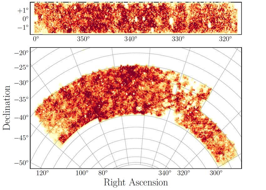
et al. 2014a,b; Applegate et al. 2014a; Hoekstra et al. 2015; Ok- Figure 1. Surface density of source galaxies in the METACALIBRATION
abe & Smith 2016; Mantz et al. 2015b; Melchior et al. 2017; Simet catalog within the DES Y1 footprint in the “S82” field (top) and the “SPT”
field (bottom).
et al. 2017; Murata et al. 2018; Dietrich et al. 2017; Miyatake et al.
2018; Medezinski et al. 2018b).
The Dark Energy Survey (DES) is a 5,000 square degree pho- compared to Melchior et al. (2017) in Section 8, and conclude in
tometric survey of the southern sky. It uses the 4-meter Blanco Tele- Section 9. In Appendix A we present the DES Y1 redMaPPer cata-
scope and the Dark Energy Camera (Flaugher et al. 2015) located log used in this work for public use. Supplementary information on
at the Cerro Tololo Inter-American Observatory. As its name sug- the analysis is given in additional appendices.
gests, the primary goal of the DES is to probe the physical nature Unless otherwise stated, we assume a flat ΛCDM cosmology
of dark energy, in addition to constraining the properties and dis- with Ωm = 0.3 and H0 = 70 km s–1 Mpc–1 , with distances defined
tribution of dark matter. Owing to its large area, depth, and image in physical coordinates, rather than comoving. Finally, unless oth-
quality, at its conclusion DES will support optical identification of erwise noted all cluster masses refer to M200m . That is, cluster mass
∼ 100, 000 galaxy clusters and groups up to redshift z ≈ 1. We use is defined as the mass enclosed within a sphere whose average den-
galaxy clusters identified using the redMaPPer algorithm (Rykoff sity is 200 times higher than the mean cosmic matter density ρ̄m
et al. 2014), which assigns each cluster a photometric redshift and at the cluster’s redshift, matching the mass definition used in the
optical richness λ of red galaxies. To fully utilize these clusters, cosmological analyses that make use of our calibration.
one must understand mass-observable relations (MORs), such as
that between cluster mass and optical richness. Weak lensing can
establish this relation – with high statistical uncertainty for individ-
ual clusters, but low systematic uncertainty in the mean mass scale 2 THE DES YEAR 1 DATA
derived from the joint signal of large samples. DES started its main survey operations in 2013, with the Year One
In this work, we use stacked weak lensing to measure the mean (Y1) observational season running from August 31, 2013 to Febru-
galaxy cluster mass of redMaPPer galaxy clusters identified in DES ary 9, 2014 (Drlica-Wagner et al. 2018). During this period 1839
Year 1 (Y1) data. We use these data to calibrate the mass–richness– deg2 of the southern sky were observed in three to four tilings in
redshift relation of these clusters. In Melchior et al. (2017) we pro- each of the four DES bands g, r, i, z, as well as ∼1800 deg2 in the
vided a first calibration of this relation using DES Science Verifica- Y-band. The resulting imaging is shallower than the SV data re-
tion (SV) data. There, we were able to achieve a 9.2 per cent statis- lease but covers a significantly larger area. In this study we utilize
tical and 5.1 per cent systematic uncertainty. Here, we update that approximately 1500 deg2 of the main survey, split into two large
result using the first year of regular DES observations, incorporat- non-contiguous areas. This is a reduction from the 1800 deg2 area
ing a variety of improvements to the analysis pipeline. Our results due to a series of veto masks. These masks include masks for bright
provide the tightest, most accurate calibration of the richness–mass stars and the Large Magellanic Cloud, among others. The two non-
relation of galaxy clusters to date, at 2.4 per cent statistical and 4.3 contiguous areas are the “SPT” area (1321 deg2 ), which overlaps
per cent systematic uncertainty. the footprint of the South Pole Telescope Sunyaev-Zel’dovich Sur-
The structure of this paper is as follows. In Section 2, we intro- vey (Carlstrom et al. 2011), and the “S82” area (116 deg2 ), which
duce the DES Y1 data used in this work. In Section 3 we describe overlaps the Stripe-82 deep field of the Sloan Digital Sky Survey
our methodology for obtaining ensemble cluster density profiles (SDSS; Annis et al. 2014). The DES Y1 footprint is shown in Fig-
from stacked weak lensing shear measurements, with a focus on up- ure 1.
dates relative to Melchior et al. (2017). A comprehensive set of tests In the following we briefly describe the main data products
and corrections for systematic effects is presented in Section 4. The used in this analysis, and refer the reader to the corresponding pa-
model of the lensing data and the inferred stacked cluster masses pers for more details. The input photometric catalog, as well as
are given in Section 5. The main result, the mass–richness–redshift the photometric redshift and weak lensing shape catalogs used in
relation of redMaPPer clusters in DES, is presented in Section 6. this study have already been employed in the cosmological analysis
We compare our results to other published works in the literature combining galaxy clustering and weak lensing by the DES collab-
in Section 7, discuss systematic improvements made in this work oration (DES Collaboration et al. 2017).
c 2017 RAS, MNRAS 000, 1–26DES Y1 WL Mass Calibration of redMaPPer Clusters 3
2.1 Photometric Catalog
Input photometry for the redMaPPer cluster finder (Section 2.2)
and photometric redshifts (Section 2.4) was derived from the DES
Y1A1 Gold catalog (Drlica-Wagner et al. 2018). Y1A1 Gold is 80
the science-quality internal photometric catalog of DES created
to enable cosmological analyses. This data set includes a cata-
log of objects as well as maps of survey depth and foreground
40
masks, and star-galaxy classification. In this work we make use
of the multi-epoch, multi-object fitting (MOF) composite model
(CM) galaxy photometry. The MOF photometry simultaneously fits
a psf-convolved galaxy model to all available epochs and bands for 20
λ
each object, while subtracting and masking neighbors. The typical
10σ limiting magnitude inside 200 diameter apertures for galaxies
in Y1A1 Gold using MOF CM photometry is g ≈ 23.7, r ≈ 23.5,
10
i ≈ 22.9, and z ≈ 22.2. Due to its low depth and calibration uncer-
tainty, we do not use Y band photometry for shape measurement or
photometric redshift estimation.
The galaxy catalog used for the redMaPPer cluster finder is 5
constructed as follows. Bad objects that are determined to be cat-
alog artifacts, including having unphysical colors, astrometric dis- 0.0 0.1 0.2 0.3 0.4 0.5 0.6 0.7 0.8
crepancies, and PSF model failures are rejected (Section 7.4 Drlica- zλ
Wagner et al. 2018). Galaxies are then selected via the more com-
plete MODEST_CLASS classifier (Section 8.1 Drlica-Wagner et al. Figure 2. Redshift–richness distribution of redMaPPer clusters in the vol-
2018). Only galaxies that are brighter in z band than the local 10 σ ume limited DES Y1 cluster catalog, overlaid with density contours to high-
limiting magnitude are used by redMaPPer. The average survey light the densest regions. At the top and on the right are histograms of the
projected quantities, zλ and λ, respectively, with smooth kernel density es-
limiting magnitude is deep enough to image a 0.2 L∗ galaxy at
timates overlaid.
z ≈ 0.7. Finally, we remove galaxies in regions that are contam-
inated by bright stars, bright nearby galaxies, globular clusters, and
the Large Magellanic Cloud.
filter method. The method allows for the inherent ambiguity of se-
lecting a central galaxy by assigning a probability to each galaxy of
being the central galaxy of the cluster. The final membership prob-
2.2 Cluster catalog
abilities of all galaxies in the field are assigned based on spatial,
We use a volume limited sample of galaxy clusters detected in the color, and magnitude filters.
DES Y1 photometric data using the redMaPPer cluster finding al- The distribution of cluster richness and redshift of the DES
gorithm v6.4.17 (Rykoff et al. 2014, 2016). This redMaPPer ver- volume-limited cluster sample is shown in Figure 2. The rich-
sion is fundamentally the same as the v6.3 algorithm described in ness estimate λ is the sum over the membership probabilities of
Rykoff et al. (2016), with minor updates. all galaxies within a pre-defined, richness–dependent projected
Two versions of the redMaPPer cluster catalog are generated: radius Rλ . The radius Rλ is related to the cluster richness via
a “flux limited” version, which includes high redshift clusters for Rλ = 1.0(λ/100)0.2 h–1 Mpc. This relation was found to mini-
which the richness requires extrapolation along the cluster lumi- mize the scatter between richness and X-ray luminosity in Rykoff
nosity function, and one that is locally volume-limited. By “locally et al. (2012). A redshift estimate for each cluster is obtained by
volume-limited” we mean that at each point in the sky, a galaxy maximizing the probability that the observed color-distribution of
cluster is included in the sample if and only if all cluster galaxies likely members matches the self-calibrated red-sequence model of
brighter than the luminosity threshold used to define cluster rich- redMaPPer.
ness in redMaPPer lies above 10 σ in z, 5 σ in i and r, and 3 σ in Figure 3 shows the photometric redshift performance of the
g according to the survey MOF depth maps (Drlica-Wagner et al. DES Y1 volume-limited redMaPPer cluster sample. The photomet-
2018). That is, no extrapolation in luminosity is required when ric redshift bias and scatter are calculated by comparing the photo-
estimating cluster richness. At the threshold the galaxy sample is metric redshift of the clusters to the spectroscopic redshift of the
> 90 – 95 per cent complete. It is this volume-limited cluster sam- central galaxy of the cluster, where available. Unfortunately, the
ple that is used in follow-up work deriving cosmological constraints small overlap with existing spectroscopic surveys means that our
from the abundance of galaxy clusters. Consequently, we focus ex- results are limited by small-number statistics: there are only 333
clusively on this volume-limited sample in this work. It contains galaxy clusters with a spectroscopic central galaxy, and only 34
more than 76,000 clusters down to λ > 5, of which more than 6,500 (six) with redshift z > 0.6 (z > 0.65). Nevertheless, the photo-
are above λ = 20. The format of the catalogs are described in Ap- metric redshift performance is consistent with our expectations: our
pendix A. redshifts are very nearly unbiased, and have a remarkably tight scat-
redMaPPer identifies galaxy clusters as overdensities of red- ter — the median value of σz /(1 + z) is ≈ 0.006. An upper limit for
sequence galaxies. Starting from an initial set of spectroscopic seed the photometric redshift bias of 0.003 is consistent with our data.
galaxies, the algorithm iteratively fits a model for the local red- Of particular importance to this work is the distribution of mis-
sequence, and finds cluster candidates while assigning a member- centered clusters – both the frequency and severity of their miscen-
ship probability to each potential member. Clusters are centered on tering. Based on the redMaPPer centering probabilities, we would
bright galaxies selected using an iteratively self-trained matched- expect ≈ 80 per cent of the clusters to be correctly centered, mean-
c 2017 RAS, MNRAS 000, 1–264 DES Collaboration
inant problem is a multiplicative bias, i.e. an over- or underestima-
0.8 Y1A1, λ > 20 tion of gravitational shear as inferred from the mean tangential el-
fout = 0.006 lipticity of lensed galaxies. This bias needs to be characterized and
0.6
corrected. Traditionally, this is done using simulated galaxy images
zspec
0.4 – with the critical limitation that simulations never fully resemble
the observations.
0.2
The METACALIBRATION catalog, in contrast, uses the galaxy
0.0 images themselves to de-bias shear estimates. Specifically, each
0.02
galaxy image is deconvolved from the estimated point spread func-
0.01 tion (PSF), and a small positive and negative shear is applied to the
zspec - zλ
deconvolved image in both the ê1 and ê2 directions. The resulting
0.00 images are then convolved once again with a representation of the
Bias PSF, and an ellipticity e is estimated for these new images (Zuntz
-0.01 σz/(1+z)
et al. 2017). These new measurements can be used to directly esti-
-0.02
mate the response of the ellipticity measurement to a gravitational
0.2 0.3 0.4 0.5 0.6 0.7 0.8
zλ shear γ using finite difference derivatives:
∂e
Figure 3. Photometric redshift performance of the DES Y1 redMaP- Rγ = . (1)
Per cluster catalog, as evaluated using available spectroscopy (333 clus-
∂γ
ters). Upper panel: Gray contours are 3σ confidence intervals, and the Selection effects can also be accounted for by examining the re-
two red dots are the only 4σ outliers, caused by miscentering on a fore- sponse of the selections to shear. The application of a weight when
ground/background galaxy. Lower Panel: photo-z bias and uncertainty. The calculating the mean shear over an ensemble is effectively a type
comparatively large uncertainty from 0.3 < z < 0.4 is due to a filter transi-
of smooth selection, and is accounted for in the same way. We de-
tion.
scribe this effect with a selection response Rsel , which leads to the
response-corrected mean shear estimate
ing the most likely redMaPPer central galaxy is at the center of
the potential well of the host halo. In practice, the fraction of cor- hγi ≈ hRi–1 hR · γtrue i ≈ hRi–1 hei (2)
rectly centered galaxy clusters is closer to ≈ 70 per cent, as es- from biased measurements e with a joint response R ≈ Rγ + Rsel
timated from a detailed comparison of the redMaPPer photomet- (Sheldon & Huff 2017). Here the left hand side represents our esti-
ric centers to the X-ray centers of redMaPPer clusters for which mate of the mean shear, while γtrue refers to the actual value.
high-resolution X-ray data is available (Zhang et al. 2018a; von der R is a 2 × 2 Jacobian matrix for the two ellipticity components
Linden et al. 2018). The expected impact of this miscentering ef- e1 , e2 in a celestial coordinate system. For the METACALIBRATION
fect, and the detailed model for the miscentered distribution from mean shear measurements in this work, we calculate the response
Zhang et al. (2018a); von der Linden et al. (2018) is described in of mean tangential shear on mean tangential ellipticity. R is close to
Section 5.2. isotropic on average, which is why other recent weak lensing anal-
yses (Troxel et al. 2017; Prat et al. 2017; Gruen et al. 2018; Chang
et al. 2018) have assumed it to be a scalar. For the larger tangential
2.3 Shear catalogs
shears measured on small scales around clusters, however, we ac-
Our work uses the DES Y1 weak lensing galaxy shape catalogs count for the fact that the response might not be quite isotropic by
presented in Zuntz et al. (2017). Two independent catalogs were explicitly rotating it to the tangential frame.
created: METACALIBRATION (Sheldon & Huff 2017; Huff & Man- The tangential ellipticity eT is related to e1 , e2 (and likewise
delbaum 2017) based on NGMIX (Sheldon 2015), and IM 3 SHAPE γT to γ1 and γ2 ) by
(Zuntz et al. 2013). Both pass a multitude of tests for systemat-
ics, making them suitable for cosmological analyses. While the Y1 eT = –e1 cos(2φ) – e2 sin(2φ) , (3)
data is shallower than the DES SV data, improvements in the shear where φ is the polar angle of the source in a coordinate system cen-
estimation pipelines and overall data quality enabled us to reach a tered on the lens. For the shear response, the corresponding rotation
number density of sources similar to that from DES SV data (Jarvis is derived from Equation 1 and Equation 3 as
et al. 2016).
In this study we will focus exclusively on the METACALI - Rγ,T = Rγ,11 cos2 (2φ) + Rγ,22 sin2 (2φ)+
(4)
BRATION shear catalog because of its larger effective source den-
Rγ,12 + Rγ,21 sin(2φ) cos(2φ) .
sity (6.28 arcmin–2 ) compared to the IM 3 SHAPE catalog (3.71
arcmin–2 ). The difference mainly arises because METACALIBRA - For the METACALIBRATION selection response, no such rotation
TION utilizes images taken in r, i, z bands, whereas IM 3 SHAPE re- can be performed as the term itself is only meaningful for ensem-
lies exclusively on r-band data. In the METACALIBRATION shear bles of galaxies. In this case, we exploit that the orientation of
catalog the fiducial shear estimates are obtained from a single source galaxies should be random relative to the clusters, which
Gaussian fit via the NGMIX algorithm. As a supplementary data suggest a symmetrized version of the response in the tangential
product METACALIBRATION provides (g, r, i, z)-band fluxes and frame:
the corresponding error estimates for objects using its internal 1 he iS+ – hei iS–
model of the galaxies. hR(T)
sel i ≈ TrhRsel i where hRsel ii,j ≈ i . (5)
2 ∆γj
Galaxy shape estimators, such as the NGMIX model-fitting
procedure used for METACALIBRATION, are subject to various In the above equation hei iS± denotes the mean un-sheared ellip-
sources of systematic errors. For a stacked shear analysis, the dom- ticity of galaxies when selected based on quantities measured on
c 2017 RAS, MNRAS 000, 1–26DES Y1 WL Mass Calibration of redMaPPer Clusters 5
their artificially sheared images. Four such sheared images are cre- where γ is the shear and κ is the convergence. In the presence of
ated by applying positive (+) and negative (–) shears of magnitude non-negligible convergence, the ellipticity estimator e introduced
∆γj = 0.01 along the j ∈ {ê1 ; ê2 } directions separately. The re- in Section 2.3 relates to the reduced shear as hgi ≈ hRi–1 hei.
sponse in the tangential and cross directions are consistent, how- The gravity of a localized mass distribution, such as a galaxy
ever both depend on the cluster-centric distance and richness of the cluster, induces positive shear along the tangential direction with
lensing clusters. These dependencies will be investigated in a future respect to the center of the overdensity. This net tangential shear
work. Errors introduced from this approximation are sub-dominant results in the stretching and preferential alignment of the images of
due to the already small bias associated with source galaxy selec- background galaxies along the tangential direction. The magnitude
tion. A detailed discussion of additional possible systematics in our of the azimuthally averaged tangential shear γT at projected radius
specific analysis is presented in Section 4.1. R can be predicted from the line-of-sight projected surface mass
density Σ of the lens mass distribution by the relation
Blinding procedure Σ(< R) – Σ(R) ∆Σ(R)
γT = ≡ . (7)
As a precaution against unintentional confirmation bias in the sci- Σcrit Σcrit
entific analyses, both weak lensing shape catalogs produced for Here Σ(< R) represents the average surface mass density within
DES Y1 had an unknown blinding factor in the magnitude of e projected radius R, and Σ(R) represents the (azimuthal) average of
(Zuntz et al. 2017) applied to them. This unknown factor was con- the surface mass density at R. For the case of reduced shear this
strained between 0.9 and 1.1. While we made initial blinded mea- equation holds only in linear order, therefore we account for the
surements for this work, the factor was revealed as part of unblind- effect of κ in our model described in Section 5.3.2.
ing the cosmology results of DES Collaboration et al. (2017). The geometry of the source–lens system modulates the ampli-
In accordance with the practices of other DES Y1 cosmology tude of the induced shear signal, and is characterized by the critical
analyses, we have further adopted a secondary layer of blinding. surface mass density
Specifically, we blindly transform the chains from our MCMCs to
hide our in-progress results, and to prevent comparison between c2 Ds
Σcrit (zs , zl ) = (8)
our cluster masses and those estimated using mass–observable re- 4πG Dl Dls
lations from the literature. Chains of the parameters in the modeled
in Equation 7. Here Ds , Dl and Dls are the angular diameter dis-
lensing profiles and the mass–richness relation were unaltered after
tances to the source, to the lens, and between the lens and the
unblinding.
source. Estimating the ∆Σ signal thus relies on robustly estimat-
ing the redshifts of the galaxy clusters and the source galaxies.
2.4 Photometric redshift catalog The lens redshifts are the photometric redshift estimates from the
redMaPPer algorithm. The statistical uncertainty on these estimates
In interpreting the weak gravitational lensing signal of galaxy clus-
is found to be ∆zl ≈ 0.01 (Rykoff et al. 2016), which is negligi-
ters as physical mass profiles we need to employ information about
ble compared to other sources of error in the lensing measurement,
the geometry of the source-lens systems by considering the relevant
allowing us to treat these redshifts as point estimates.
angular-diameter distances. To calculate these distances we rely on
Source redshifts are also estimated from photometry, and are
estimates of the overall redshift distribution of source galaxies, and
described by a probability distribution pphot (zs ) for each source
also on information about the individual P(z) of source galaxies.
galaxy. We can therefore only estimate an effective critical surface
We use the DES Y1 photometric redshifts estimated and val-
density
idated by Hoyle et al. (2017) using the template-based BPZ algo- Z
rithm (Benítez 2000; Coe et al. 2006). It was found by Hoyle et al.
hΣ–1crit ii,j = dzs pphot (zs,i ) Σ–1
crit (zl,j , zs,i ) , (9)
(2017) that these photo-z estimates were modestly biased, introduc-
ing an overall multiplicative systematic correction in the recovered
where i and j index the source and the lens in a lens-source pair.
weak lensing profiles. We determine this correction and its system-
Note that here we choose to express the inverse critical surface
atic uncertainty in Section 4.3.
density, which is the predicted amplitude of the lensing signal in
In order to be able to correct selection effects due to the change
Equation 7. We consistently define it as zero if zs 6 zl . For reasons
of photo-z with shear while utilizing the highest signal-to-noise
of data compression, we will in fact not use the full integral over
flux measurements for determining the source redshift distribution,
pphot (z) later, but rather replace Equation 9 by Σ–1
crit evaluated at a
we use two separate BPZ catalogs: one generated from META -
random sample of the pphot (z).
CALIBRATION -measured photometry (for selecting and weighting
sources), and one from MOF (see Section 2.1) photometry (for de-
termining the resulting source redshift distributions). Details of this
are described in the following section. 3.1.1 The lensing estimator
Due to the low signal-to-noise of individual source-lens pairs we
measure the stacked (mean) signal of many source galaxies around
3 STACKED LENSING MEASUREMENTS a selection of clusters.
3.1 Mass density profiles Sheldon et al. (2004) show that the minimum variance estima-
tor for the weak lensing signal is
Gravitational lensing induces distortions in the images of back-
lens src .
ground “source” galaxies. In the limit of weak gravitational lensing, PP
wi,j eT; i,j hΣ–1
crit ii,j
these are characterized by the “reduced shear” j i
∆Σ
g= , (10)
γ
P
wi,j
g≡ , (6) j,i
1–κ
c 2017 RAS, MNRAS 000, 1–266 DES Collaboration
where the summation goes over all source–lens pairs in some radius to use the METACALIBRATION photo-z estimates only for select-
bin and eT; i,j is the tangential component of the ellipticity of source ing and weighting source-lens pairs. When normalizing the shear
i relative to lens j.DThe optimal
E weights, proportional to the inverse signal to find ∆Σ, we utilize the MOF-based photo-z estimates.
variance of eT; i,j / Σ–1crit , are
. 3.1.3 Data vector binned in redshift and richness
wi,j = hΣ–1 2 2
crit ii,j σγ,i , (11)
In estimating the lensing signal through Equation 12 we utilize a
2
where σγ,i is the estimate on the variance of the measured shear modified version of the publicly available XSHEAR code1 and the
estimate of galaxy i relating to both the intrinsic variance of shapes custom built XPIPE python package.2 The core implementation of
and also to the uncertainty originating from shear estimation. the measurement code is identical to the one used by Melchior et al.
(2017).
We group the clusters into three bins in redshift: z ∈ [0.2; 0.4),
3.1.2 Practical lensing estimator [0.4; 0.5), and [0.5; 0.65), as well as seven bins in richness: λ ∈
This estimator can be equivalently understood as a mean tangential [5; 10), [10; 14), [14; 20), [20; 30), [30; 45), [45; 60), and [60; ∞).
ellipticity, weighted by the expected shear signal amplitude of each The redshift limit z = 0.65 of our highest redshift corresponds
galaxy hΣ–1 crit i. It is normalized by the expected signal per unit ∆Σ,
roughly to the highest redshift for which the redMaPPer cluster cat-
i.e. the hΣ–1 –1 alog remains volume limited across the full DES Y1 survey foot-
crit i-weighted mean of the hΣcrit i. With this in mind, and
including shear and selection response (see Section 2.3), we define print. The ∆Σ profiles were measured in 15 logarithmically spaced
the estimator we use in practice as radial bins ranging from 0.03 Mpc to 30 Mpc. For our later results
P we will only utilize the radial range above 200 kpc. Scales below
ωi,j eT; i,j this cut are included only in our figures and for reference purposes,
j,i
g ≡
∆Σ ! . (12) and are excluded from the analysis to avoid systematic effects such
P 0 –1 T
ωi,j Σcrit;i,j Rγ,i +
P 0 –1 T
ωi,j Σcrit;i,j hRsel i as obscuration, significant membership contamination, and blend-
j,i j,i ing. This radial binning scheme yields similar S/N across all bins.
The measured shear profiles are shown in Figure 4.
In the above, hRTsel i is calculated via Equation 5 separately for We find a mild radial dependence in the typical value for
source galaxies selected in each radial bin and each richness – METACALIBRATION shear response hRγ,T i, the asymptotic values
redshift bin, where the corresponding selections were defined by are 0.6, 0.58 and 0.55 as a function of increasing cluster redshift.
the photometric redshift estimates derived from the sheared META - For the selection response we find an asymptotic value of hRsel i ≈
CALIBRATION photometries. The small number of source galax- 0.013, 0.014, and 0.015.
ies at small radii introduces some noise to the estimated response,
however due to the intrinsic environmental dependence of RTsel , this
cannot be readily substituted or approximated with other, less noisy 3.2 Covariance matrices
quantities. By considering the expectation value
The ∆Σ profiles estimated in the previous section deviate from the
heT; i,j i = ∆Σ Σ–1 T
crit;i,j Ri , (13) true signal due to statistical uncertainties and systematic biases. We
construct a description for the covariance of our data vector below
it is easy to see that the definition of Equation 12 yields an unbiased and calibrate the influence of systematic effects in Section 4.
estimate of ∆Σ. Statistical uncertainties originate from the large intrinsic scat-
Equation 12 includes two simplifications to make calculations ter in the shapes of source galaxies, the uncertainty in estimating
less computationally demanding. First, for the normalization, we their photometric redshifts, and due to the intrinsic variations in
replace the expectation value of Σ–1 crit by a Monte Carlo estimate the properties and environments of galaxy clusters. Furthermore,
0
–1 our typical maximum radii: 2, 1.5 and 1.3 degrees for the different
Σcrit;i,j = Σcrit (zlj , zMC
si ) , (14)
redshift ranges respectively are much larger than the 0.22 degree
where zMC
si is a random sample from the pphot (zs ) distribution esti-
median separation between clusters in the catalog. This means that
mated with BPZ using MOF photometry. Second, the weights are source galaxies are paired with multiple clusters, possibly generat-
chosen as ing covariance between different radial ranges and/or across differ-
ent cluster bins in richness and redshift.
ωi,j ≡ Σ–1 MCAL
crit zlj , hzsi i if hzMCAL
si i > zlj + ∆z , (15) To quantify the correlation and uncertainty involved in the
measurement we construct a semi-analytic model for the data co-
with hzMCAL
s i being the mean redshift of the source galaxy es- variance matrix following the framework developed by Gruen et al.
timated from METACALIBRATION photometry. Given the width (2015). Our use of a semi-analytic covariance (SAC) matrix is mo-
of our photometrically estimated p(z), this is close to the opti- tivated by explicit covariance estimators exhibiting non-negligible
mal weight. We use a padding of ∆z = 0.1 for source selection. uncertainty and possible biases, for instance from jackknife regions
We found that including the source weights provided by META - that are not completely independent. Both of these problems lead
CALIBRATION does not introduce a significant improvement in the to a biased estimate of the precision matrix (i.e. the inverse covari-
signal-to-noise of the measurement. ance matrix), which in turn will bias the posteriors of likelihood
The use of two different photometric estimators is necessary inference (Friedrich et al. 2016).
because when calculating the selection response, the internal pho- Instead, we predict several key contributions of the observed
tometry of the METACALIBRATION, with measurements on sheared covariances, namely those due to correlated and uncorrelated large
images, must be used for all selection and weighting of sources.
Hoyle et al. (2017) find this photometric redshift estimate to have a 1 https://github.com/esheldon/xshear
greater scatter than the default MOF photometry. We therefore opt 2 https://github.com/vargatn/xpipe
c 2017 RAS, MNRAS 000, 1–26DES Y1 WL Mass Calibration of redMaPPer Clusters 7
103 z ∈ [0.2; 0.35) z ∈ [0.2; 0.35) z ∈ [0.2; 0.35) z ∈ [0.2; 0.35) z ∈ [0.2; 0.35) z ∈ [0.2; 0.35) z ∈ [0.2; 0.35)
λ ∈ [5; 10) λ ∈ [10; 14) λ ∈ [14; 20) λ ∈ [20; 30) λ ∈ [30; 45) λ ∈ [45; 60) λ ∈ [60; ∞)
102
101
100
Nclus = 10636 Nclus = 2089 Nclus = 1375 Nclus = 762 Nclus = 376 Nclus = 123 Nclus = 91
z ∈ [0.35; 0.5) z ∈ [0.35; 0.5) z ∈ [0.35; 0.5) z ∈ [0.35; 0.5) z ∈ [0.35; 0.5) z ∈ [0.35; 0.5) z ∈ [0.35; 0.5)
∆Σ [ M /pc2 ]
3
10
λ ∈ [5; 10) λ ∈ [10; 14) λ ∈ [14; 20) λ ∈ [20; 30) λ ∈ [30; 45) λ ∈ [45; 60) λ ∈ [60; ∞)
102
101
100
Nclus = 18331 Nclus = 4135 Nclus = 2612 Nclus = 1549 Nclus = 672 Nclus = 187 Nclus = 148
10 3 z ∈ [0.5; 0.65) z ∈ [0.5; 0.65) z ∈ [0.5; 0.65) z ∈ [0.5; 0.65) z ∈ [0.5; 0.65) z ∈ [0.5; 0.65) z ∈ [0.5; 0.65)
λ ∈ [5; 10) λ ∈ [10; 14) λ ∈ [14; 20) λ ∈ [20; 30) λ ∈ [30; 45) λ ∈ [45; 60) λ ∈ [60; ∞)
102
101
100
Nclus = 22991 Nclus = 4974 Nclus = 2927 Nclus = 1612 Nclus = 687 Nclus = 205 Nclus = 92
10−1 100 101 10−1 100 101 10−1 100 101 10−1 100 101 10−1 100 101 10−1 100 101 10−1 100 101
R [Mpc]
Figure 4. Mean ∆Σ for cluster subsets split in redshift zl (increasing from top to bottom) and λ (increasing from left to right), as labeled. The error bars shown
are the diagonal entries of our semi-analytic covariance matrix estimate (see Section 3.2) for bins with λ > 20 and the jackknife estimated covariance matrix
for bins with λ < 20. The best-fit model (red curve) is shown for bins with λ > 20, and includes dilution from cluster member galaxies (Section 5.3.1) and
miscentering (Section 5.2); see Section 5 for details. Semi-analytic covariances were not computed for stacks with λ < 20 due to the significant computational
cost. Below 200 kpc we consider data points unreliable and therefore exclude them from our analysis; these are indicated by open symbols and dashed lines.
The profiles and jackknife errors are calculated after the subtraction of the random-point shear signal (see Section 4.1.3).
scale structure, stochasticity in cluster centering, the intrinsic scat- 1.00
ter in cluster concentrations at fixed mass, cluster ellipticity, and −1.0 z ∈ [0.20; 0.35) z ∈ [0.20; 0.35) 0.75
the scatter in the richness–mass relation of galaxy clusters. Only λ ∈ [20; 30) λ ∈ [20; 30) 0.50
−0.5
the shape noise contribution is estimated directly from the data, as × 0.25
0.0 λ ∈ [30; 45)
detailed below. 0.00
While we rely on the SAC matrix estimates in the remainder 0.5 −0.25
of our analysis, we compare the SAC matrices to those derived us- −0.50
log10R [Mpc]
1.0
ing a standard jackknife method. We use jackknife (JK) resampling −0.75
with K = 100 simply-connected spatial regions Rk selected via a −1.00
−1.0 −0.5 0.0 0.5 1.0
k-means algorithm on the sphere.3 The jackknife covariance is de- −1.0
fined following Efron (1982): log10R [Mpc]
−0.5
K T
K – 1 X g g (·) · ∆Σ
0.0
g =
C∆Σ ∆Σ(k) – ∆Σ g (k) – ∆Σ
g (·) , (16)
K 0.5 z ∈ [0.20; 0.35)
k
×
g (·) = 1 P ∆Σ 1.0 z ∈ [0.35; 0.50)
where ∆Σ K k
g (k) and ∆Σ
g (k) denotes the lensing signal
λ ∈ [20; 30)
estimated via Equation 12 using all lenses except those in region
−1.0 −0.5 0.0 0.5 1.0
Rk . Using this method, we calculate the covariance between all
radial bins in a single richness and redshift bin, as well as the co- log10R [Mpc]
variance between adjacent richness and redshift bins.
Figure 5 shows an example of the structure of the jackknife Figure 5. Jackknife estimated correlation matrix of ∆Σ g of a single
estimated correlation matrix between neighboring bins in rich- richness-redshift selection with λ ∈ [20; 30) and z ∈ [0.2; 0.35) (upper
ness and redshift. We find no significant correlation between rich- left panel). The off-diagonal blocks display the correlation matrix between
the reference profile and the neighboring richness bin λ ∈ [30; 45) (upper
ness/redshift bin and therefore treat each bin independently, even
right panel), and the neighboring redshift bin z ∈ [0.35; 0.5) (lower left
though some systematic parameters may be shared between bins.
panel)
3.2.1 Shape noise from both the random intrinsic alignments and also the stochas-
The large intrinsic variations of the shapes of galaxies (shape noise) tic positions of source galaxies. In order to do so, we make use of
in the source catalog constitute a dominant source of uncertainty the measurement setup outlined in Section 3.1.3, but each source
in lensing measurements. We estimate the covariance originating is randomly rotated to create a new source catalog. We generated
1000 such independent rotated source catalogs, and performed the
3 https://github.com/esheldon/kmeans_radec lensing measurement with each. The resulting data vectors are con-
c 2017 RAS, MNRAS 000, 1–268 DES Collaboration
sistent with zero, as the random rotation washes away the imprint halos of mass M a distance R from the halo is
of the weak lensing signal. However, their scatter is indicative of dn
ρh (M, Rh ) = b(Mcl )b(M)wmm (Rh ) , (18)
the covariance due to shape noise. dM
We estimate the shape noise covariance matrix for each of the where wmm is the projected linear correlation function at the red-
1000 realizations using the spatial jackknife scheme outlined above shift of the cluster, b(M) is the halo bias, and dn/dM is the halo
in Section 3.2. The final shape noise covariance matrix estimate is mass function, or the number of halos per unit volume per unit
obtained by averaging all 1000 of these jackknife covariance matri- mass (Tinker et al. 2008).
ces. We expect this method to be less noisy compared to estimating Given a model for the halo profile Σ(R|M), the contribution of
the covariance matrix from the 1000 independent measurements of a halo at location Rh to the mean surface density Σ of the cluster in
the rotated ∆Σ vector only. radial bin Ri is Σi (M, Rh ) = Σmisc (Ri |M, Rh ), where Σmisc is a mis-
centered halo profile. Because of the Poisson-sampling assumption,
the covariance matrix is generated by the mass profiles of individ-
3.2.2 Uncorrelated LSS ual halos, so that the correlated large scale structure contribution to
the covariance matrix can be written as
Line of sight structures which are not physically connected to the Z
cluster leave an impact on the lensing signal. We cannot remove CijcLSS = (2πRh dRh )dM ρh (M, Rh )∆Σi (M, Rh )∆Σj (M, Rh ) .
them from the signal, but we can estimate their expected contribu- (19)
tion to the covariance. For an individual cluster, the covariance of In practice, the above predicted covariance matrix is further
the ∆Σ profile at radii θi , θj due to uncorrelated large scale struc- rescaled by a constant factor calibrated on simulations. This is
ture (uLSS) can be written as (e.g. Schneider et al. 1998; Hoekstra meant to account for additional variance not captured by linear bias
2003; Umetsu et al. 2011) and Poisson noise, due to filamentary structure and higher order
Z statistics in the spatial distribution of the correlated halos (e.g. the
`d`
CijuLSS = hΣ–1
crit i
–2
Pκ (`)J2 (`θi )J2 (`θj ) , (17) non-zero three-point function). A more detailed derivation of the
2π
above equation and its calibration is found in Gruen et al. (2015).
where Pκ is the power spectrum of the convergence, and J2 is the A very similar calculation can be made for characterizing the
Bessel function of the first kind of order 2. contribution due to halo ellipticity (to the covariance matrix – for
Naively, one would expect that the variance of a cluster the effect on the mean signal, see Section 5.4.2). If ρell (q, µ) is the
stack due to uncorrelated large scale structure to scale simply as distribution of the halo axis ratio q and the line-of-sight orientation
1/Nclusters . In practice, however, the positions of galaxy clusters are angle θ relative to the major axis such that cos θ = µ, then one finds
correlated, and the area around them overlaps on large scales. Con- (Gruen et al. 2015)
sequently, we expect the variance due to uncorrelated structure to
Z
decrease somewhat more slowly than 1/Nclusters . Cijell = dqdµ ρell (q, µ)∆Σi ∆Σj , (20)
We estimate this source of noise by measuring random realiza-
where ∆Σi is the contribution to the bin Ri under the assumption
tions of the signal due to shear fields induced by log-normal density
that the halo has an axis ratio q and an orientation µ.
fields with the appropriate power spectra and skewness. We calcu-
late the latter with the perturbation theory model of Friedrich et al.
(2017) for the Buzzard cosmology (DeRose et al. 2018; Wechsler 3.2.4 M–c scatter, M-λ scatter and miscentering
et al. 2018), using the log-normal parameter κ0 at a 10’ aperture
Halos at a given mass have some intrinsic scatter in their M–λ rela-
radius. As our cluster sample spans a range in redshift, a different
tion. A rough estimate of the intrinsic scatter in the mass–richness
shear field is calculated for each of the three redshift bins. This is
(M–λ) relation is ∼ 25 per cent (Rozo & Rykoff 2014; Farahi et al.
done such that the shear fields are calculated at the lens-weighted
2018), and it causes an increase in the variance of stacked mea-
mean source galaxy redshifts found during the initial measurement
surements of ∆Σ. This scatter causes an even larger increase in
in Section 3.1.3. We then pass these shear fields through the mea-
the variance, since it propagates into quantities that depend directly
surement pipeline using a spatial mask reflecting the actual source
on the mass, including the M – c relation. In addition, concentra-
number density variations across the footprint, and estimate the co-
tion (e.g. Diemer & Kravtsov 2015; Bhattacharya et al. 2013) and
variance matrix for each realizations using 100 spatial jackknife
miscentering possess some intrinsic scatter from halo to halo them-
regions for each bin in richness and redshift.
selves.
This above procedure was repeated 300 times, and the final
Scatter in the M–λ relation causes variance on all scales, since
covariance matrix due to uncorrelated LSS is taken to be the mean
the bias b(M) directly depends on the mass. By comparison, scatter
of the 300 jackknife covariance estimates.
in the M – c relation primarily affects small scales where the 1-halo
term dominates. Similarly, some cluster centers are misidentified
in our stacks, which creates additional covariance at small scales
3.2.3 Correlated LSS and halo ellipticity where the signal is substantially suppressed.
We modeled the combined contribution to the SAC from scat-
Following Gruen et al. (2015), we model correlated large scale
ter in M–λ, scatter in concentration at fixed mass, and miscentering
structure using a halo model approach. We assume correlated halos
of individual clusters in our stacks by doing the following:
can be adequately described using only two parameters: the mass
M of the correlated halo, and the projected distance Rh from the (i) For each cluster in our stack, assign a mass by inverting a fidu-
cluster. The mass distribution of the halos is assumed to follow the cial M–λ relation (Melchior et al. 2017) and assuming 25 per cent
halo mass function, while their spatial distribution is modeled as scatter. This is not identical to 25 per cent scatter in the M–λ rela-
a Poisson realization of the density field defined by the appropri- tion, however this choice negligibly affects this component of the
ate halo–cluster correlation function. That is, the excess density of covariance matrix.
c 2017 RAS, MNRAS 000, 1–26DES Y1 WL Mass Calibration of redMaPPer Clusters 9
(ii) For each cluster, assign a concentration (including scatter) based Shape Noise cLSS+ell
on Diemer & Kravtsov (2015).
(iii) For each cluster, make a draw from our centering prior described 1.0
log10 R [Mpc]
in Section 5.2. In other words, some fraction fmis of clusters in the 0.5 103
stack are miscentered, and the distribution of the amount of mis- 0.0
centering is given by p(Rmis ). 102
-0.5
(iv) Calculate ∆Σ for each cluster and average these signals to gener- 101
ate a signal for the entire stack. -1.0
[M /pc2 ]2
(v) Repeat this process many times, and use these independent real- 100
izations to estimate the corresponding covariance matrix between M-c+M-λ+Mis uLSS
the various radial bins. 10−1
1.0
log10 R [Mpc]
Using Simet et al. (2017) as our fiducial M–λ relation or using the 0.5 10−2
Bhattacharya et al. (2013) mass–concentration relation had no im- 0.0
10−3
pact on the final SAC matrix. We have also verified that using half -0.5
as many realizations as our fiducial choice (1000) did not appre- -1.0 10−4
ciably change the resulting covariance matrix. The same is true for
changes in the richness scatter or miscentering model parameters -1.0 -0.5 0.0 0.5 1.0 -1.0 -0.5 0.0 0.5 1.0
within reasonable ranges. log10 R [Mpc] log10 R [Mpc]
Figure 6. The four individual components to our Semi-Analytic Covari-
ance (SAC) matrix. Clockwise from top left: Shape noise component from
randomly rotating sources, correlated LSS and ellipticity component from
integrating over configurations of the host cluster and its correlated halos,
3.2.5 Semi-analytic covariance matrix uncorrelated LSS from integrating over large scale structure, and finally
scatter in the M – λ relation, M – c relation, and miscentering distribution.
Following Gruen et al. (2015), the full SAC matrix is obtained by Dark colors correspond to low covariance and the colors are log scaled to
adding each of the above contributions. The individual components show trends. Light colors are normalized to the total covariance in the SAC.
described in the previous subsections are shown in Figure 6. Fig- See Section 3.2 for details.
ure 7 demonstrates the differences between the SAC and jackknife
covariance matrices. The top two panels show the correlation ma-
4 SYSTEMATICS
trix R of the SAC and CJK respectively, where the correlation ma-
trix is defined via 4.1 Shear systematics
Cij The METACALIBRATION shear catalog and the associated calibra-
Rij = p . (21) tion of the source redshift distributions (Hoyle et al. 2017) passed
Cii Cjj
a large number of tests performed by Zuntz et al. (2017) and Prat
et al. (2017). Here we briefly enumerate the constraints on the most
Similarly, to visualize the difference between CSA and CJK we de- relevant systematics, and refer the reader to the corresponding pa-
fine the residual matrix pers for a more detailed analysis.
We parametrize the various potential biases in the dataset as:
CijSA – CijJK
Qij = q . (22) gi = (1 + mi )gtri + αPSF ePSF
i + ci , (23)
CiiSA CjjSA
where gtri
is the true shear, while gi is the shear estimate, and αPSF
relates to the contamination from the PSF ellipticity ePSF
i .
We show this residual matrix in the bottom right panel of Figure 7. In weak lensing surveys the three main sources of bias are
Finally, in the lower left panel we show the difference between the commonly found to be model bias, noise bias, and selection bias
errors along the diagonal between the CJK and the SAC, along with (or representativeness bias). In order to account and correct for
each of the contributions to the SAC; the lower panel shows the these sources of error, the METACALIBRATION algorithm performs
fractional difference between the diagonal entries. As expected, a self-calibration on the actual data by shearing the galaxy im-
shape noise is the dominant contributor to the SAC matrix, with ages during the measurement, and using the thus calculated re-
uncorrelated LSS becoming important at the largest scales. This sponses to correct the shear estimates. To quantify the effectiveness
explains why the choices we had to make in modeling the non- of this self-calibration, Zuntz et al. (2017) ran the METACALIBRA -
shape noise components did not significantly affect the resulting TION pipeline on a set of simulated galaxy images using G AL S IM
SAC matrix or the posteriors analysis. (Rowe et al. 2015). The images were produced from high resolu-
Using the SACs in our analysis provides two major improve- tion galaxy images from the COSMOS sample, and processed to
ments: minimal bias from inverting the covariance matrix, and less resemble the actual DES Y1 observations both in noise and PSF
overall noise in the off-diagonal elements which improves the mass properties. Based on this test scenario Zuntz et al. (2017) found no
measurement. In Melchior et al. (2017) we demonstrated that noise significant multiplicative bias m or additive bias c present in the
in the jackknife covariance matrix led to an increase of ≈30 per dataset.
cent in the uncertainty of the mass of the stack. Using the SACs Zuntz et al. (2017) further investigated the multiplicative bi-
reduces the contribution of the covariance to the error budget by 10 ases due to blending of galaxy images, due to the potential leak-
per cent compared to the jackknife estimated covariance. age of stellar objects into the galaxy sample, and due to poten-
c 2017 RAS, MNRAS 000, 1–2610 DES Collaboration
RSA RJK
1.00
1.0
log10 R [Mpc]
0.5 0.75
0.0
0.50
-0.5
-1.0 0.25
-1.0 -0.5 0.0 0.5 1.0
0.00
log10 R [Mpc] Q
JK
103
SAC
−0.25
σ∆Σ [M /pc2 ]
Shape
102 uLSS
cLSS+ell
101 M-c+M-λ+Mis
−0.50
100
10−1
−0.75
0.5
JK−SAC
SAC
0.0
−1.00
−0.5
10−1 100 101 -1.0 -0.5 0.0 0.5 1.0
R [Mpc] log10 R [Mpc]
Figure 7. Comparison between the semi-analytic covariance matrix and the jackknife estimated covariance matrix. Top left: Correlation matrix of the SAC
matrix. Top-right: Correlation matrix of the jackknife estimate. Bottom left: Comparison of the errors in the SAC and jackknife estimate along with the
contributions to the SAC error from each individual component. The line showing the SAC errors lies almost on top of the shape noise contribution, confirming
that it is the dominant source of covariance. Bottom right: Residual matrix Q (see Equation 22) that represents the difference between the SAC and jackknife
covariance matrices. See Section 3.2 for details.
tial errors in the modeling of the PSF. They found blending as the term, at third order in γt = ∆Σ × Σ–1 crit , as
only component with a net bias, with the other sources being con- 3
sistent with zero, although contributing to the uncertainty on the ∆Σobs hΣ–1 crit i – αNL ∆ΣModel hΣ–1
crit i
value of m. The final multiplicative bias estimates were found to be ∆Σ0obs = , (24)
hΣ–1
crit i
m = [1.2 ± 1.3] · 10–2 with a 1σ Gaussian error. They found no
evidence of a significant additive bias term. where ∆ΣModel is the optimized model discussed in Section 5. For
Prat et al. (2017) tested for the presence of residual shear cal- the amplitude of non-linear shear bias we choose αNL = 0.6 (Shel-
ibration biases in the DES Y1 galaxy-galaxy lensing analysis by don & Huff 2017). We model the profile of the highest richness
splitting the source sample by various galaxy properties and pa- stack at z ∈ [0.2, 0.35] where, for the source redshift distribution
rameters of the observational data. They showed that within the of DES Y1, this effect is strongest. The recovered mass changes
statistical uncertainty of the respective galaxy-galaxy lensing sig- by less than 1 per cent, demonstrating that our recovered mass–
nals, and including the differences in redshift distributions induced richness–redshift relation is robust to non-linear shear bias within
by the splitting, no differential multiplicative biases between any of our error budget.
the splits are significantly detected. The choice of α = 0.6 in our test is motivated by the image
In addition to the above calibrations during the construction of simulations used in Sheldon & Huff (2017). Other simulations find
the shear catalog, we perform additional sanity checks relevant to a range of values of similar magnitude. Since the effect is smaller
stacked weak lensing measurements in the subsections below. than the overall shear uncertainty, yet its calibration is uncertain,
we choose not to implement a correction in our final model.
4.1.1 Second order shear bias
4.1.2 B-modes
Due to the larger tangential shear near massive clusters, this analy-
sis is more strongly affected by non-linear shear response than pre- Gravitational lensing due to localized mass distributions can only
vious DES Y1 lensing analyses (see the discussion in section 9 of produce a net E-mode signal in the shear field, which corresponds
Sheldon & Huff 2017). This response biases cluster masses higher to the tangential shear γt . This allows for a simple null test for the
than they would be otherwise. To test this effect, we modify the presence of systematics: any non-zero cross-shear (i.e. a non-zero
measured ∆Σ profiles by adding the leading non-linear shear bias B-mode) must be due to systematics. We compute the cross-shear
c 2017 RAS, MNRAS 000, 1–26You can also read