Euclid preparation: XI. Mean redshift determination from galaxy - export.arXiv.org
←
→
Page content transcription
If your browser does not render page correctly, please read the page content below
Astronomy & Astrophysics manuscript no. paper                                                                                           ©ESO 2021
                                              January 8, 2021

                                                   Euclid preparation: XI. Mean redshift determination from galaxy
                                                         redshift probabilities for cosmic shear tomography
                                               Euclid Collaboration: O. Ilbert1? , S. de la Torre1 , N. Martinet1 , A.H. Wright2 , S. Paltani3 , C. Laigle4 , I. Davidzon5 ,
                                               E. Jullo1 , H. Hildebrandt2 , D.C. Masters6 , A. Amara7 , C.J. Conselice8 , S. Andreon9 , N. Auricchio10 , R. Azzollini11 ,
                                                C. Baccigalupi12,13,14,15 , A. Balaguera-Antolínez16,17 , M. Baldi10,18,19 , A. Balestra20 , S. Bardelli10 , R. Bender21,22 ,
                                                A. Biviano12,15 , C. Bodendorf22 , D. Bonino23 , S. Borgani12,14,15,24 , A. Boucaud25 , E. Bozzo3 , E. Branchini26,27,28 ,
                                                M. Brescia29 , C. Burigana30,31,32 , R. Cabanac33 , S. Camera23,34,35 , V. Capobianco23 , A. Cappi10,36 , C. Carbone37 ,
                                               J. Carretero38 , C.S. Carvalho39 , S. Casas40 , F.J. Castander41,42 , M. Castellano28 , G. Castignani43 , S. Cavuoti29,44,45 ,
                                                A. Cimatti18,46 , R. Cledassou47 , C. Colodro-Conde17 , G. Congedo48 , L. Conversi49,50 , Y. Copin51 , L. Corcione23 ,
                                                    A. Costille1 , J. Coupon3 , H.M. Courtois51 , M. Cropper11 , J. Cuby1 , A. Da Silva52,53 , H. Degaudenzi3 , D. Di
arXiv:2101.02228v1 [astro-ph.CO] 6 Jan 2021

                                                    Ferdinando19 , F. Dubath3 , C. Duncan54 , X. Dupac50 , S. Dusini55 , A. Ealet56 , M. Fabricius21,22 , S. Farrens40 ,
                                                    P.G. Ferreira54 , F. Finelli10,30 , P. Fosalba41,42 , S. Fotopoulou57 , E. Franceschi10 , P. Franzetti37 , S. Galeotta15 ,
                                                      B. Garilli37 , W. Gillard58 , B. Gillis48 , C. Giocoli10,18,19 , G. Gozaliasl59 , J. Graciá-Carpio22 , F. Grupp21,22 ,
                                                     L. Guzzo9,60,61 , S.V.H. Haugan62 , W. Holmes63 , F. Hormuth64 , K. Jahnke65 , E. Keihanen66 , S. Kermiche58 ,
                                                       A. Kiessling63 , C.C. Kirkpatrick66 , M. Kunz67 , H. Kurki-Suonio66 , S. Ligori23 , P. B. Lilje62 , I. Lloro68 ,
                                                  D. Maino37,60,61 , E. Maiorano10 , O. Marggraf69 , K. Markovic63 , F. Marulli10,18,19 , R. Massey70 , M. Maturi71,72 ,
                                                       N. Mauri18,19 , S. Maurogordato36 , H. J. McCracken4 , E. Medinaceli73 , S. Mei74 , R.Benton Metcalf18,73 ,
                                                  M. Moresco10,18 , B. Morin75,76 , L. Moscardini10,18,19 , E. Munari15 , R. Nakajima69 , C. Neissner38 , S. Niemi11 ,
                                                     J. Nightingale77 , C. Padilla38 , F. Pasian15 , L. Patrizii19 , K. Pedersen78 , R. Pello1 , V. Pettorino40 , S. Pires40 ,
                                               G. Polenta79 , M. Poncet47 , L. Popa80 , D. Potter81 , L. Pozzetti10 , F. Raison22 , A. Renzi55,82 , J. Rhodes63 , G. Riccio29 ,
                                                    E. Romelli15 , M. Roncarelli10,18 , E. Rossetti18 , R. Saglia21,22 , A.G. Sánchez22 , D. Sapone83 , P. Schneider69 ,
                                                T. Schrabback69 , V. Scottez4 , A. Secroun58 , G. Seidel65 , S. Serrano41,42 , C. Sirignano55,82 , G. Sirri19 , L. Stanco55 ,
                                                   F. Sureau40 , P. Tallada Crespí84 , M. Tenti19 , H. I. Teplitz6 , I. Tereno39,52 , R. Toledo-Moreo85 , F. Torradeflot84 ,
                                                    A. Tramacere3 , E.A. Valentijn86 , L. Valenziano10,19 , J. Valiviita66,87 , T. Vassallo21 , Y. Wang6 , N. Welikala48 ,
                                                                J. Weller21,22 , L. Whittaker8,88 , A. Zacchei15 , G. Zamorani10 , J. Zoubian58 , E. Zucca10
                                                                                                 (Affiliations can be found after the references)
                                                                                                       Received on date, accepted on date

                                                                                                                   ABSTRACT

                                              The analysis of weak gravitational lensing in wide-field imaging surveys is considered to be a major cosmological probe of dark energy. Our ca-
                                              pacity to constrain the dark energy equation of state relies on the accurate knowledge of the galaxy mean redshift hzi. We investigate the possibility
                                              of measuring hzi with an accuracy better than 0.002 (1 + z), in ten tomographic bins spanning the redshift interval 0.2 < z < 2.2, the requirements
                                              for the cosmic shear analysis of Euclid. We implement a sufficiently realistic simulation to understand the advantages, complementarity, but also
                                              shortcoming of two standard approaches: the direct calibration of hzi with a dedicated spectroscopic sample and the combination of the photometric
                                              redshift probability distribution function (zPDF) of individual galaxies. We base our study on the Horizon-AGN hydrodynamical simulation that
                                              we analyse with a standard galaxy spectral energy distribution template-fitting code. Such procedure produces photometric redshifts with realistic
                                              biases, precision and failure rate. We find that the Euclid current design for direct calibration is sufficiently robust to reach the requirement on the
                                              mean redshift, provided that the purity level of the spectroscopic sample is maintained at an extremely high level of > 99.8%. The zPDF approach
                                              could also be successful if we debias the zPDF using a spectroscopic training sample. This approach requires deep imaging data, but is weakly
                                              sensitive to spectroscopic redshift failures in the training sample. We improve the debiasing method and confirm our finding by applying it to
                                              real-world weak-lensing data sets (COSMOS and KiDS+VIKING-450).
                                              Key words. photometric redshift – spectroscopic and imaging surveys – methods: observational – techniques: photometric

                                              1. Introduction                                                              potheses are: a modification of the laws of gravity, the introduc-
                                                                                                                           tion of a cosmological constant Λ in the equations describing the
                                              Understanding the late, accelerated expansion of our Universe                dynamics of our Universe, or the existence of a dark energy fluid
                                              (Riess et al. 1998; Perlmutter et al. 1999) is one of the most               with negative pressure. The two latter hypotheses could be disen-
                                              important challenges in modern cosmology. Three leading hy-                  tangled one from another by measuring the equation of state w of
                                                                                                                           dark energy, which links its pressure to its density. Only the case
                                               ?
                                                   e-mail: olivier.ilbert@lam.fr

                                                                                                                                                                       Article number, page 1 of 21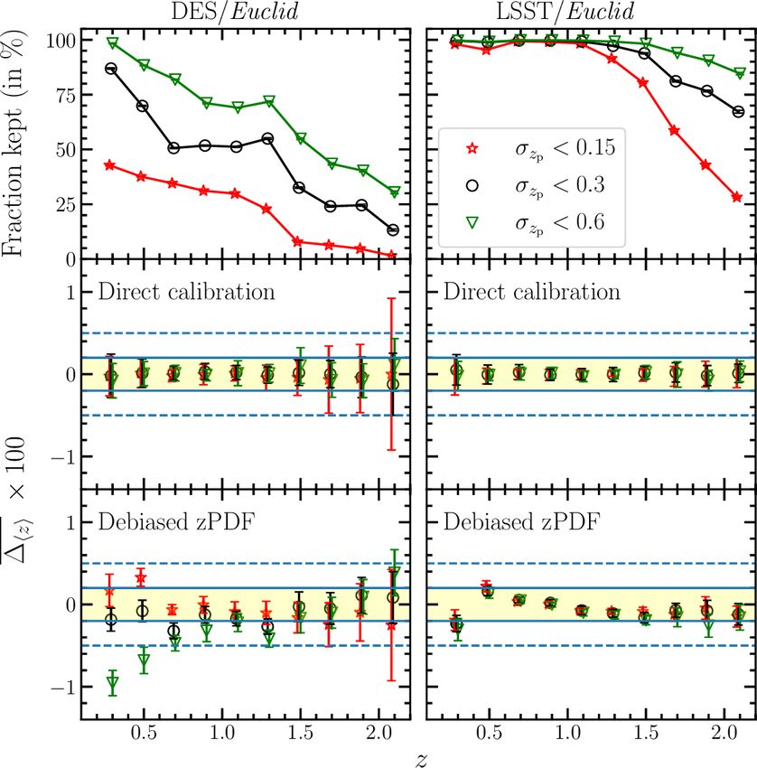
A&A proofs: manuscript no. paper

w = −1 is compatible with a cosmological constant, and there-         However these photo-z are imperfect (due to, for example, pho-
fore any deviation from this value would invalidate the standard      tometric noise), resulting in tomographic bins whose true N(z)
Λ cold dark matter (ΛCDM) model, in favour of dark energy.            extend beyond the bin limits. These ‘tails’ in the redshift distri-
This makes the precise measurement of w a key component of            bution are important, as they can significantly influence the dis-
future cosmological experiments such as Euclid (Laureijs et al.       tribution mean and bring sensitive information (Ma et al. 2006).
2011), the Vera C. Rubin Observatory Legacy Survey of Space           For a Euclid-like cosmic shear survey, Laureijs et al. (2011) pre-
and Time (LSST; LSST Science Collaboration et al. 2009), or           dict that the mean redshift hzi of each tomographic bin must be
the Nancy Grace Roman Space Telescope (Spergel et al. 2015).          known with an accuracy better than σhzi = 0.002 (1 + z) in order
     Cosmic shear (see e.g. Kilbinger 2015; Mandelbaum 2018,          to meet the precision on w0 (σw0 = 0.015) and wa (σwa = 0.15).
for recent reviews), which is the coherent distortion of galaxy           Given the importance of measuring the mean redshift for
images by large-scale structures via weak gravitational lensing,      cosmic-shear surveys, numerous approaches have been devised
offers the potential to measure w with great precision: the Eu-       in the last decade. A first family of methods, usually referred to
clid survey, in particular, aims at reaching 1% precision on the      as ‘direct calibration’, involves weighting a sample of galaxies
measurement of w using cosmic shear. One advantage of using           with known redshifts such that they match the colour-magnitude
lensing to measure w, compared to other probes, is that there ex-     properties of the target galaxy sample; thereby leveraging the
ists a direct link between galaxy image geometrical distortions       relationship between galaxy colours, magnitudes, and redshifts
(i.e. the shear) and the gravitational potential of the intervening   to reconstruct the redshift distribution of the target sample (e.g.
structures. When the shapes of, and distances to, galaxy sources      Lima et al. 2008; Cunha et al. 2009; Abdalla et al. 2008).
are known, gravitational lensing allows one to probe the matter       A second approach is to utilise redshift probability distribu-
distribution of the Universe.                                         tion functions (zPDFs), obtained per target galaxy and subse-
     This discovery has led to the rapid growth of interest in us-    quently stacked them to reconstruct the target population N(z).
ing cosmic shear as a key cosmological probe, as evidenced            The galaxy zPDF is typically estimated by either model fitting
by its successful application to several surveys. Constraints on      or via machine learning. A third family of methods uses galaxy
the matter density parameter Ωm , and the normalisation of the        spatial information, specifically galaxy angular clustering, cross-
linear matter power spectrum σ8 , have been reported by the           correlating target galaxies with a large spec-z sample to retrieve
Canada-France-Hawaii Telescope Lensing Survey (CFHTLenS,              the redshift distribution (e.g. Newman 2008; Ménard et al. 2013).
Kilbinger et al. 2013), the Kilo Degree Survey (Hildebrandt           New methods are continuously developed, for instance by mod-
et al. 2017, KiDS,), the Dark Energy Survey (DES, Troxel et al.       elling galaxy populations and using forward modelling to match
2018), and the Hyper-Suprime Camera Survey (HSC, Hikage               the data (Kacprzak et al. 2020).
et al. 2019). These studies typically utilise so-called cosmic            In this paper we evaluate our capacity to measure the mean
shear tomography (Hu 1999), whereby the cosmic shear signal           redshift in each tomographic bin at the precision level required
is obtained by measuring the cross-correlation between galaxy         for Euclid, based on realistic simulations.
shapes in different bins along the line of sight (i.e. tomographic        We base our study on a mock catalogue generated from
bins). Large forthcoming surveys, also utilising cosmic shear to-     the Horizon-AGN hydrodynamical simulation as described in
mography, will enhance the precision of cosmological param-           Dubois et al. (2014) and Laigle et al. (2019). The advantage of
eter measurements (e.g. Ωm , σ8 , and w), while also enabling         this simulation is that the produced spectra encompass all the
the measurement of any evolution in the dark-energy equation          complexity of galaxy evolution, including rapidly varying star-
of state, such as that parametrised by Caldwell et al. (1998):        formation histories, metallicity enrichment, mergers, and feed-
w = w0 + wa (1 − a), where a is the scale factor.                     back from both supernovae and active galactic nuclei (AGN).
     Tomographic cosmic shear studies require accurate knowl-         By simulating galaxies with the imaging sensitivity expected for
edge of the galaxy redshift distribution. The estimation and cal-     Euclid, we retrieve the photo-z with a standard template-fitting
ibration of the redshift distribution has been identified as one      code, as done in existing surveys. Therefore, we produce photo-
of the most problematic tasks in current cosmic shear surveys,        z with realistic biases, precision and failure rate, as shown in
as systematic bias in the distribution calibration directly influ-    Laigle et al. (2019). The simulated galaxy zPDF appear as com-
ences the resulting cosmological parameter estimates. In partic-      plex as the ones observed in real data.
ular, Joudaki et al. (2020) show that the Ωm −σ8 constraints from         We further simulate realistic spectroscopic training samples,
KiDS and DES can be fully reconciled under consistent redshift        with selection functions similar with those that are currently be-
calibration, thereby suggesting that the different constraints from   ing acquired in preparation of Euclid and other dark energy ex-
the two surveys can be traced back to differing methods of red-       periments (Masters et al. 2017). We introduce possible incom-
shift calibration.                                                    pleteness and failures as occurring in actual spectroscopic sur-
     In tomographic cosmic shear, the signal is primarily sensitive   veys.
to the average distance of sources within each bin. Therefore,            We investigate two of the methods envisioned for the Euclid
for this purpose, the redshift distribution of an arbitrary galaxy    mission: the direct calibration and zPDF combination. We also
sample can be characterised simply by its mean hzi, defined as:       propose a new method to debias the zPDF based on Bordoloi
                                                                      et al. (2010). We quantify their performance to estimate the mean
        R∞
               z N(z) dz                                              redshift of tomographic bins, and isolate relevant factors which
hzi =   R0 ∞               ,                                   (1)    could impact our ability to fulfill the Euclid requirement. We
          0
               N(z) dz                                                also provide recommendations on the imaging depth and training
                                                                      sample necessary to achieve the required accuracy on hzi.
where N(z) is the true redshift distribution of the sample. Fur-          Finally, we demonstrate the general utility of each of the
thermore, in cosmic shear tomography it is common to build the        methods presented here, not just to future surveys such as Eu-
required tomographic bins using photo-z (see Salvato et al. 2019,     clid but also to current large imaging surveys. As an illustration,
for a review), which can be measured for large samples of galax-      we apply those methods to COSMOS and the fourth data release
ies with observations in only a few photometric bandpasses.           of KiDS (Kuijken et al. 2019) surveys.
Article number, page 2 of 21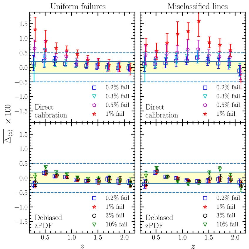
Euclid Collaboration: O. Ilbert et al.: Determination of the mean redshift of tomographic bins

    The paper is organised as follows. In Sect. 2 we describe
the Euclid-like mock catalogues generated from the Horizon-
AGN hydrodynamical simulation. In Sect. 3 we test the precision
reached on hzi when applying the direct calibration method. In
Sect. 4 we measure hzi in each tomographic bin using the zPDF
debiasing technique. We discuss the advantages and limitations
of both methods in Sect. 5. We apply these methods to the KiDS
and COSMOS data set in Sect. 6. Finally, we summarise our
findings and provide closing remarks in Sect. 7.

2. A Euclid mock catalogue
                                                                        Fig. 1. Comparison between the photometric redshifts (zp ) and spec-
In this section we present the Euclid mock catalogue used in            troscopic redshifts (zs ) for the Horizon-AGN simulated galaxy sam-
this analysis, which is constructed from the Horizon-AGN hy-            ple. Each panel shows a two-dimensional histogram with logarithmic
drodynamical simulated lightcone and includes photometry and            colour scaling, and is annotated with both the 1:1 equivalence line (red)
                                                                        and |zp − zs | = 0.15 (1 + zs ) outlier thresholds (blue), for reference.
photometric redshift information. A full description of this mock
                                                                        Photometric redshifts are computed using both DES/Euclid (left) and
catalogue can be found in Laigle et al. (2019). Here we sum-            LSST/Euclid (right) simulated photometry, assuming a Euclid-based
marise its main features and discuss the construction of several        magnitude limited sample with V IS < 24.5.
simulated spectroscopic samples, which reproduce a number of
expected spectroscopic selection effects.
                                                                        the final catalogue, resulting in more than 7 × 10⁵ galaxies in the
2.1. Horizon-AGN simulation                                             redshift range 0 < z < 4, with a spatial resolution of 1 kpc.
Horizon-AGN is a cosmological hydrodynamical simulation ran                  A full description of the per-galaxy spectral energy distri-
in a simulation box of 100 h−1 Mpc per-side, and with a dark            bution (SED) computation within Horizon-AGN is presented in
matter mass resolution of 8 × 10⁷ M (Dubois et al. 2014). A flat        Laigle et al. (2019)1 , in the following we only summarise the
ΛCDM cosmology with H0 = 70.4 km s−1 Mpc−1 , Ωm = 0.272,                key details of the SED construction process. Each stellar par-
ΩΛ = 0.728, and ns = 0.967 (compatible with WMAP-7, Ko-                 ticle in the simulation is assumed to behave as a single stellar
matsu et al. 2011) is assumed. Gas evolution is followed on an          population, and its contribution to the galaxy spectrum is gen-
adaptive mesh, whereby an initial coarse 10243 grid is refined          erated using the stellar population synthesis models of Bruzual
down to 1 physical kpc. The refinement procedure leads to a             & Charlot (2003), assuming a Chabrier (2003) initial mass func-
typical number of 6.5 × 10⁹ gas resolution elements (called leaf        tion. As each galaxy is composed of a large number of stellar
cells) in the simulation at z = 1. Following Haardt & Madau             particles, the galaxy SEDs therefore naturally capture the com-
(1996), heating of the gas by a uniform ultra-violet background         plexities of unique star-formation and chemical enrichment his-
radiation field takes place after z = 10. Gas in the simulation         tories. Additionally, dust attenuation is also modelled for each
is able to cool down to temperatures of 104 K through H and             star particle individually, using the mass distribution of the gas-
He collision, and with a contribution from metals as tabulated          phase metals as a proxy for the dust distribution, and adopting
in Sutherland & Dopita (1993). Gas is converted into stellar            a constant dust-to-metal mass ratio. Dust attenuation (neglect-
particles in regions where the gas particle number density sur-         ing scattering) is therefore inherently geometry-dependent in the
passes n0 = 0.1 H cm−3 , following a Schmidt law, as explained          simulation. Finally, absorption of SED photons by the intergalac-
in Dubois et al. (2014). Feedback from stellar winds and super-         tic medium (i.e. Hi absorption in the Lyman-series) is modelled
novae (both types Ia and II) are included in the simulation, and        along the line of sight to each galaxy, using our knowledge of
include mass, energy, and metal releases. Black holes (BHs) in          the gas density distribution in the lightcone. This therefore intro-
the simulation can grow by gas accretion, at a Bondi accretion          duces variation in the observed intergalactic absorption across
rate that is capped at the Eddington limit, and are able to coalesce    individual lines of sight. Flux contamination by nebular emis-
when they form a sufficiently tight binary. They release energy         sion lines is not included in the simulated SEDs. While emission
in either the quasar or radio (i.e. heating or jet) mode, when the      lines could add some complexity in galaxy’s photometry, their
accretion rate is respectively above or below one per cent of the       contribution could be modelled in template-fitting code. More-
Eddington ratio. The efficiency of these energy release modes           over, their impact is mostly crucial at high redshift (Schaerer &
are tuned to match the observed BH-galaxy scaling relation at           de Barros 2009) and when using medium bands (e.g. Ilbert et al.
z = 0 (see Dubois et al. 2012, for more details).                       2009).
     The simulation lightcone was extracted as described in Pi-              Kaviraj et al. (2017) compare the global properties of the
chon et al. (2010). Particles and gas leaf cells were extracted at      simulated galaxies with statistical measurements available in the
each time step depending on their proper distance to the observer       literature (as the luminosity functions, the star-forming main se-
at the origin. In total, the lightcone contains roughly 22 000 por-     quence, or the mass functions). They find an overall fairly good
tions of concentric shells, which are taken from about 19 replica-      agreement with observations. Still, the simulation over-predicts
tions of the Horizon-AGN box up to z = 4. We restrict ourselves         the density of low-mass galaxies, and the median specific star
to the central 1 deg2 of the lightcone. Laigle et al. (2019) ex-        formation rate falls slightly below the literature results, a com-
tracted a galaxy catalogue from the stellar particle distribution       mon trend in current simulations.
using the AdaptaHOP halo finder (Aubert et al. 2004), where
galaxy identification is based exclusively on the local stellar par-
ticle density. Only galaxies with stellar masses M? > 109 M              1
                                                                           Horizon-AGN photometric catalogues and SEDs can be downloaded
(which corresponds to around 500 stellar particles) are kept in         from https://www.horizon-simulation.org/data.html

                                                                                                                   Article number, page 3 of 21
A&A proofs: manuscript no. paper
Fig. 2. Few examples of galaxy likelihood L (z) (dashed red lines) and debiased posterior distributions (solid black lines). The spec-z (photo-z)
are indicated with green (magenta) dotted lines. These galaxies are selected in the tomographic bin 0.4 < zp < 0.6 for the DES/Euclid (top panels)
and LSST/Euclid (bottom panels) configurations. These likelihoods are not a random selection of sources, but illustrate the variety of likelihoods
present in the simulations.
2.2. Simulation of Euclid photometry and photometric and even then it is possible that the northern extension of LSST
redshifts might not reach the same depth. Still, LSST will be already ex-
tremely deep after two years of operation, being only 0.9 magni-
As described in Laureijs et al. (2011), the Euclid mission will tude shallower than the final expected sensitivity (Graham et al.
measure the shapes of about 1.5 billion galaxies over 15 000 2020). Therefore, these two cases (and their assumed sensitivi-
deg2 . The visible (VIS) instrument will obtain images taken in ties) should comfortably encompass the possible photo-z perfor-
one very broad filter (V IS ), spanning 3500 Å. This filter allows mance of any future combined optical and Euclid photometric
extremely efficient light collection, and will enable VIS to mea- data set.
sure the shapes of galaxies as faint as 24.5 mag with high pre- In order to generate the mock photometry in each of the
cision. The near infrared spectrometer and photometer (NISP) Euclid, DES, and LSST surveys, each galaxy SED is first ‘ob-
instrument will produce images in three near-infrared (NIR) fil- served’ through the relevant filter response curves. In each pho-
ters. In addition to these data, Euclid satellite observations are tometric band, we generate Gaussian distributions of the ex-
expected to be complemented by large samples of ground-based pected signal-to-noise ratios (SNs) as a function of magnitude,
imaging, primarily in the optical, to assist the measurement of given both the depth of the survey and typical SN-magnitude re-
photo-z. lation (in the same wavelength range) (see appendix A in Laigle
Euclid imaging has an expected sensitivity, over 15 000 deg2 , et al. 2019). We then use these distributions, per filter, to assign
of 24.5 mag (at 10σ) in the V IS band, and 24 mag (at 5σ) in each each galaxy a SN (given its magnitude). The SN of each galaxy
of the Y, J, and H bands (Laureijs et al. 2011). We associate the determines its ‘true’ flux uncertainty, which is then used to per-
Euclid imaging with two possible ground-based visible imaging turb the photometry (assuming Gaussian random noise) and pro-
datasets, which correspond to two limiting cases for photo-z es- duce the final flux estimate per source. This process is then re-
timation performance. peated for all desired filters.
– DES/Euclid. As a demonstration of photo-z performance The galaxy photo-z are derived in the same manner as with
when combining Euclid with a considerably shallower pho- real-world photometry. We use the method detailed in Ilbert et al.
tometric dataset, we combine our Euclid photometry with (2013), based on the template-fitting code LePhare (Arnouts
that from DES (Abbott et al. 2018). DES imaging is taken in et al. 2002; Ilbert et al. 2006). We adopt a set of 33 templates
the g, r, i, and z filters, at 10σ sensitivities of 24.33, 24.08, from Polletta et al. (2007) complemented with templates from
23.44, and 22.69 respectively. Bruzual & Charlot (2003). Two dust attenuation curves are con-
– LSST/Euclid. As a demonstration of photo-z performance sidered (Prevot et al. 1984; Calzetti et al. 2000), allowing for
when combining Euclid with a considerably deeper photo- a possible bump at 2175Å. Neither emission lines nor adap-
metric dataset, we combine our Euclid photometry with that tation of the zero-points are considered, since they are not in-
from the Vera C. Rubin Observatory LSST (LSST Science cluded in the simulated galaxy catalogue. The full redshift like-
Collaboration et al. 2009). LSST imaging will be taken in lihood, L (z), is stored for each galaxy, and the photo-z point-
the u, g, r, i, z, and y filters, at 5σ (point source, full depth) estimate, zp , is defined as the median of L (z)2 . The distribu-
sensitivities of 26.3, 27.5, 27.7, 27.0, 26.2, and 24.9, respec- tions of (derived) photometric redshift versus (intrinsic) spectro-
tively. scopic redshift for mock galaxies (in both our DES/Euclid and
DES imaging is completed and meets these expected sensitiv- 2
The median of L (z) could differ from the peak of L (z), or from
ities. Conversely LSST will not reach those quoted full depth the redshift corresponding to the minimum χ2 , especially for ill-defined
sensitivities before its tenth year of operation (starting in 2021), likelihoods.
Article number, page 4 of 21Euclid Collaboration: O. Ilbert et al.: Determination of the mean redshift of tomographic bins
LSST/Euclid configurations) are shown in Fig. 1. Several ex- ESO and Keck facilities (Masters et al. 2019; Guglielmo et al.
amples of redshift likelihoods are shown in Fig. 2. We can see 2020). The target selection is based on an unsupervised machine-
realistic cases with multiple modes in the distribution, as well learning technique, the self-organising map (SOM, Kohonen
as asymmetric distributions around the main mode. The photo-z 1982), which they use to define a spectroscopic target sample
used to select galaxies within the tomographic bins are indicated that is representative in terms of galaxy colours of the Euclid
by the magenta lines and that they can differ significantly from cosmic shear sample. The SOM allows a projection of a multi-
the spec-z (green lines). dimensional distribution into a lower two-dimensional map. The
We wish to remove galaxies with a broad likelihood distribu- utility of the SOM lies in its preservation of higher-dimensional
tion (i.e. galaxies with truly uncertain photo-z) from our sample. topology: neighbouring objects in the multi-dimensional space
In practice, we approximate the breadth of the likelihood distri- fall within similar regions of the resulting map. This allows
bution using the photo-z uncertainties produced by the template- the SOM to be utilised as a multi-dimensional clustering tool,
fitting procedure to clean the sample. LePhare produces a red- whereby discrete map cells associate sources within discrete
p , zp ], per source, which encom-
shift confidence interval [zmin max voxels in the higher dimensional space. We utilise the method
passes 68% of the redshift probability around zp . We remove of Davidzon et al. (2019) to construct a SOM, which involves
p , zp − zp ) > 0.3, which we de-
galaxies with max( zp − zmin max projecting observed (i.e. noisy) colours of the mock catalogue
note σzp > 0.3 in the following for simplicity. We investigate into a map of 6400 cells (with dimension 80 × 80). We construct
the impact of this choice on the number of galaxies available for our SOM using the LSST/Euclid simulated colours, assuming
cosmic shear analyses, and also quantify the impact of relaxing implicitly that the spec-z training sample is defined using deep
this limit, in Sect. 5.2. calibration fields. If the flux uncertainty is too large (∆mix > 0.5,
Finally, we generate 18 photometric noise realisations of the for object i in filter x) the observed magnitude is replaced by
mock galaxy catalogue. While the intrinsic physical properties that predicted from the best-fit SED template, which is estimated
of the simulated galaxies remain the same under each of these while preparing the SOM input catalogue. This procedure allows
realisations, the differing photometric noise allows us to quan- us to retain sources that have non-detections in some photomet-
tify the role of photometric noise alone on our estimated of hzi. ric bands. We then construct our SOM-based training sample by
We only adopt 18 realisations due to computational limitations, randomly selecting Ntrain galaxies from each cell in the SOM.
however, our results are stable to the addition of more realisa- The C3R2 expects to have > 1 spectroscopic galaxies per SOM
tions. cell available for calibration by the time that the Euclid mission
is active. For our default SOM coverage, we invoke a slightly
more idealised situation of two galaxies per cell and we impose
2.3. Definition of the target photometric sample and the that these two galaxies belong to the considered tomographic
spectroscopic training samples bin. This procedure ensures that all cells are represented in the
All redshift-calibration approaches discussed in this paper utilise spectroscopy. In reality, a fraction of cells will likely not con-
a spec-z training sample to estimate the mean redshift of a target tain spectroscopy. However, when treated correctly, such mis-
photometric sample. In practice, such a spectroscopic training represented cells act only to decrease the target sample num-
sample is rarely a representative subset of the target photomet- ber density, and do not bias the resulting redshift distribution
ric sample, but is often composed of bluer and brighter galaxies. mean estimates (Wright et al. 2020). We therefore expect that
Therefore, to properly assess the performance of our tested ap- this idealised treatment will not produce results that are overly-
proaches, we must ensure that the simulated training sample is optimistic.
distinct from the photometric sample. To do this, we separate the
Horizon-AGN catalogue into two equal sized subsets: we define Finally, the COSMOS-like training sample mimics a typi-
the first half of the photometric catalogue as our as target sample, cal heterogeneous spectroscopic sample, currently available in
and draw variously defined spectroscopic training samples from the COSMOS field. We first simulate the zCOSMOS-like spec-
the second half of the catalogue. We test each of our calibration troscopic sample (Lilly et al. 2007), which consists of two dis-
approaches with three spectroscopic training samples, designed tinct components: a bright and a faint survey. The zCOSMOS-
to mimic different spectroscopic selection functions: Bright sample is selected such that it contains only galaxies at
z < 1.2, while the zCOSMOS-Faint sample contains only galax-
– a uniform training sample; ies at z > 1.7 (with a strong bias towards selecting star-forming
– a SOM-based training sample; galaxies). To mimic these selections, we construct a mock sam-
– and a COSMOS-like training sample. ple whereby half of the sources are brighter than i = 22.5 (the
bright sample) and half of the galaxies reside at 1.7 < z < 2.4
The uniform training sample is the simplest, most idealised with g < 25 (the faint sample). We then add to this compilation
training sample possible. We sample 1000 galaxies with V IS < a sample of 2000 galaxies that are randomly selected at i < 25,
24.5 mag (i.e. the same magnitude limit as in the target sample) mimicking the low-z VUDS sample (Le Fevre et al. 2015), and
in each tomographic bin, independently of all other properties. a sample of 1000 galaxies randomly selected at 0.8 < z < 1.6
While this sample is ideal in terms of representation, the sample with i < 24, mimicking the sample of Comparat et al. (2015).
size is set to mimic a realistic training sample that could be ob- By construction, this final spectroscopic redshift compilation ex-
tained from dedicated ground-based spectroscopic follow-up of hibits low representation of the photometric target sample in the
a Euclid-like target sample. redshift range 1.3 < z < 1.7.
Our second training sample follows the current Euclid base-
line to build a training sample. Masters et al. (2017) endeavour
to construct a spectroscopic survey, the Complete Calibration of Overall, our three training samples exhibit (by design) dif-
the Colour-Redshift Relation survey (C3R2), which completely fering redshift distributions and galaxy number densities. We in-
samples the colour/magnitude space of cosmic shear target sam- vestigate the sensitivity of the estimated hzi on the size of the
ples. This sample is currently assembled by combining data from training sample in Sect. 5.3.
Article number, page 5 of 21A&A proofs: manuscript no. paper
target sample. The method relies on the assumption that galaxies
within a cell share the same redshift (Masters et al. 2015) which
can be labelled with the training sample. Therefore, we can es-
timate the mean redshift of the target distribution hzi by simply
calculating the weighted mean of each cell’s average redshift,
where the weight is the number of target galaxies per cell:
Ncells D
1 X E
hzi = zitrain Ni , (2)
Nt i=1
where
D E the sum runs over the i ∈ [1, Ncells ] cells in the SOM,
zitrain is the mean redshift of the training spectroscopic sources
in cell i, Ni is the number of target galaxies (per tomographic bin)
in cell i, and Nt is the total number of target galaxies in the tomo-
graphic bin. A shear weight associated to each galaxy can be in-
troduced in this equation (e.g. Wright et al. 2020). As described
in Sect. 2.3, our SOM is consistently constructed by training
on LSST/Euclid photometry, even when studying the shallower
DES/Euclid configuration. We adopt this strategy since the train-
ing spectroscopic samples in Euclid will be acquired in calibra-
tion fields (e.g. Masters et al. 2019) with deep dedicated imag-
ing. This assumption implies that the target distribution hzi is
estimated exclusively in these calibration fields, which are cov-
ered with photometry from both our shallow and deep setups,
and therefore increases the influence of sample variance on the
calibration.
The COSMOS-like sample. Applying direct calibration to
a heterogeneous training sample is less straightforward than in
the above cases, as the training sample is not representative of
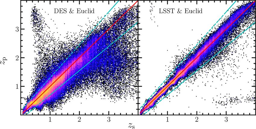
Fig. 3. Bias on the mean redshift (see Eq. 3) averaged over the 18 pho- the target sample in any respect. Weighting of the spectroscopic
tometric noise realisations. The mean redshifts are measured using the sample, therefore, must correct for the mix of spectroscopic se-
direct calibration approach. The tomographic bins are defined using lection effects present in the training sample, as a function of
the DES/Euclid and LSST/Euclid photo-z in the top and bottom pan- magnitude (from the various magnitude limits of the individ-
els, respectively. The yellow region represents the Euclid requirement ual spectroscopic surveys), colour (from their various preselec-
at 0.002 (1 + z) for the mean redshift accuracy, and the blue dashed lines tions in colour and spectral type), and redshift (from dedicated
correspond to a bias of 0.005 (1 + z). The symbols represent the results redshift preselection, such as that in zCOSMOS-Faint). Such a
obtained with different training samples: (a) selecting uniformly 1000 weighting scheme can be established efficiently with machine-
galaxies per tomographic bin (black circles); (b) selecting two galax- learning techniques such as the SOM. To perform this weight-
ies/cell in the SOM (red squares); and (c) selecting a sample that mim-
ing, we train a new SOM using all the information that have
ics real spectroscopic survey compilations in the COSMOS field (green
triangles). the potential to correct for the selection effects present in our
heterogeneous training sample: apparent magnitudes, colours,
and template-based photo-z. We create this SOM using only the
3. Direct calibration galaxies from the COSMOS-like sample that belong to the con-
sidered tomographic bin, and reduce the size of the map to 400
Direct calibration is a fairly straightforward method that can be cells (20 × 20, because the tomographic bin itself spans a smaller
used to estimate the mean redshift of a photometric galaxy sam- colour space). Finally, we project the target sample into the SOM
ple, and is currently the baseline method planned for Euclid cos- and derive weights for each training sample galaxy, such that
mic shear analyses. In this section we describe our implemen- they reproduce the per-cell density of target sample galaxies.
tation of the direct calibration method, apply this method to our This process follows the same weighting procedure as Wright
various spectroscopic training samples, and report the resulting et al. (2020), who extend the direct calibration method of Lima
accuracy of our redshift distribution mean estimates. et al. (2008) to include source groupings defined via the SOM.
In this method, the estimate of hzi is also inferred using Eq. (2).
3.1. Implementation for the different training samples
3.2. Results
Given our different classes of training samples, we are able to
implement slightly different methods of direct calibration. We We apply the direct calibration technique to the mock catalogue,
detail here how the implementation of direct calibration differs split into ten tomographic bins spanning the redshift interval
for each of our three spectroscopic training samples. 0.2 < zp < 2.2. To construct the samples within each tomo-
The uniform sample. In the case where the training sample graphic bin, training and target samples are selected based on
is known to uniformly sparse-sample the target galaxy distribu- their best-estimate photo-z, zp . We quantify the performance of
tion, an estimate of hzi can be approximated by simply comput- the redshift calibration procedure using the measured bias in hzi,
ing the mean redshift of the training sample. defined as:
The SOM sample. By construction, the SOM training sam- hzi − hzitrue
ple uniformly covers the full n-dimensional colour space of the ∆hzi = , (3)
1 + hzitrue
Article number, page 6 of 21Euclid Collaboration: O. Ilbert et al.: Determination of the mean redshift of tomographic bins
and evaluated over the target sample. We present the values of Poisson noise dominates over sample variance (in mean redshift
∆hzi that we obtain with direct calibration in Fig. 3, for each of estimation) when the training sample consists of less than 100
the ten tomographic bins. The figure shows, per tomographic galaxies. Above this size, sample variance dominates the cali-
bin, the population mean (points) and 68% population scatter bration uncertainty. This means that, in order to generate an un-
(error bars) of ∆hzi over the 18 photometric noise realisations of biased estimate of hzi using a uniform sample of 1000 galaxies,
our simulation. The solid lines and yellow region indicate the a minimum of 10 fields of 2 deg2 would need to be surveyed.
|∆hzi | ≤ 2 × 10⁻³ requirement stipulated by the Euclid mission. The SOM approach is less sensitive to sample variance, as
Given our limited number of photometric noise realisations, es- over-densities (and under-densities) in the target sample popu-
timating the population mean and scatter directly from the 18 lation relative to the training sample are essentially removed in
samples is not sufficiently robust for our purposes. We thus use the weighting procedure (provided that the population is present
maximum likelihood estimation, assuming Gaussianity of the in the training sample, Lima et al. 2008; Wright et al. 2020).
∆hzi distribution, to determine the underlying population mean In the cells corresponding to this over-represented target popu-
and the scatter. We define these underlying population statistics lation, the relative importance of training sample redshifts will
as µ∆z and σ∆z for the mean and the scatter, respectively. be similarly up-weighted, thereby removing any bias in the re-
We find that, when using a uniform or SOM training sam- constructed N(z). Therefore, sample variance should have only a
ple, direct calibration is consistently able to recover the target weak impact on the global derived N(z) in this method. Nonethe-
sample mean redshift to |µ∆z | < 2 × 10⁻³ . In the case of the less, samples variance may still be problematic if, for example,
shallow DES/Euclid configuration, however, the scatter σ∆z ex- under-densities result in entire populations being absent from the
ceeds the Euclid accuracy requirement in the highest and lowest training sample.
tomographic bins. The DES/Euclid configuration is, therefore, Finally, it is worth emphasising that these results are ob-
technically unable to meet the Euclid precision requirement on tained assuming perfect knowledge of training set redshifts. We
hzi in the extreme bins. In the LSST/Euclid configuration, con- study the impact of failures in spectroscopic redshift estimation
versely, the precision and accuracy requirements are both consis- in Sect. 5.
tently satisfied. We hypothesise that this difference stems from
the deeper photometry having higher discriminatory power in
the tomographic binning itself: the N(z) distribution for each to- 4. Estimator based on redshift probabilities
mographic bin is intrinsically broader for bins defined with shal-
In this section we present another approach to redshift distribu-
low photometry, and therefore has the potential to demonstrate
tion calibration that uses the information contained in the galaxy
greater complexity (such as colour-redshift degeneracies) that re-
redshift probability distribution function, available for each in-
duce the effectiveness of direct calibration.
dividual galaxy of the target sample. Photometric redshift esti-
The direct calibration with the SOM relies on the assump-
mation codes typically provide approximations to this distribu-
tion that galaxies within a cell share the same redshift (Masters
tion based solely on the available photometry of each source.
et al. 2015). Noise and degeneracies in the colour-redshift space
We study the performance of methods utilising this information
introduce a redshift dispersion within the cell which impacts the
in the context of Euclid and test a method to debias the zPDF.
accuracy of hzi. Even with the diversity of SED generated with
Horizon-AGN, and introducing noise in the photometry, we find
that the direct calibration with a SOM sample is sufficient to 4.1. Formalism
reach the Euclid requirement.
We find that the COSMOS-like training sample is unable to Given the relationship between galaxy magnitudes and colours
reach the required accuracy of Euclid. This behaviour is some- (denoted o) and redshift z, one can utilise the conditional proba-
what expected, since the COSMOS-like sample contains selec- bility p(z|o) to estimate the true redshift distribution N(z), using
tion effects that are not cleanly accessible to the direct calibration an estimator such as that of Sheth (2007); Sheth & Rossi (2010):
weighting procedure. The mean redshift is particularly biased in
the bin 1.6 < z < 1.8, where there is a dearth of spectra; the Z Nt
Comparat et al. (2015) sample is limited to z < 1.6, while the
X
N(z) = N(o) p(z|o) do = pi (z|o), (4)
zCOSMOS-Faint sample resides exclusively at z > 1.7, thereby i
leaving the range 1.6 < z < 1.7 almost entirely unrepresented.
In this circumstance, our SOM-based weighting procedure is in- where N(o) is the joint n-dimensional distribution of colours
sufficient to correct for the heterogeneous selection, leading to and magnitudes. As made explicit in the above equation, the
bias. This is typical in cases where the training sample is missing N(z) estimator reduces simply to the sum of the individual (per-
certain galaxy populations that are present in the target sample galaxy) conditional redshift probability distributions, pi (z|o). A
(Hartley et al. 2020). We note, though, that it may be possible to shear weight associated to each galaxy can be introduced in this
remove some of this bias via careful quality control during the equation (e.g. Wright et al. 2020). It is worth noting that this
direct calibration process, such as demonstrated in Wright et al. summation over conditional probabilities is ideologically similar
(2020). Whether such quality control would be sufficient to meet to the summation of SOM-cell redshift distributions presented
the Euclid requirements, however, is uncertain. previously; in both cases, one effectively builds an estimate of
We note that, although we are utilising photometric noise re- the probability p(z|o), and uses this to estimate hzi. Indeed, it is
alisations in our estimates of hzi, the underlying mock catalogue clear that the SOM-based estimate of hzi presented in Eq. (2) in
remains the same. As a result, our estimates of µ∆z and σ∆z are fact follows directly from Eq. (4).
not impacted by sample variance. In reality, sample variance af- Generally, photometric redshift codes provide in output a
fects the performance of the direct calibration, particularly when normalised likelihood function that gives the probability of the
assuming that the training sample is directly representative of the observed photometry given the true redshift, L (o|z), or some-
target distribution (as we do with our uniform training sample). times the posterior probability distribution P(z|o) (e.g. Benítez
For fields smaller than 2 deg2 , Bordoloi et al. (2010) showed that 2000; Bolzonella et al. 2000; Arnouts et al. 2002; Cunha et al.
Article number, page 7 of 21A&A proofs: manuscript no. paper
Fig. 4. Examples of redshift distributions (left) and PIT distributions (right, see text for details) for a tomographic bin selected to 0.8 < zp < 1
using DES/Euclid photo-z. In these examples, we assume a training sample extracted from a SOM, with two galaxies per cell. The top and bottom
panels show the results before and after zPDF debiasing, respectively. Redshift distributions and PITs are shown for the true redshift distribution
(blue), and redshift distributions estimated using the zPDF method, when incorporating photo-z (red) and uniform (black) priors.
2009). These two probability distribution functions are related Pr(T |m0 ) is the prior conditional probability of each template at
through the Bayes theorem as, a given reference magnitude. Under the approximation that the
redshift distribution does not depend on the template, and that
P(z|o) ∝ L (o|z) Pr(z), (5) the template distribution is independent of the magnitude (i.e.
where Pr(z) is the prior probability. the luminosity function does not depend on the SED type), one
Photometric redshift methods that invoke template-fitting, obtains
X
such as the LePhare photo-z estimation code, generally explore P(z|c, m0 ) ∝ L (c|T, z) Pr(z|m0 ) (8)
the likelihood of the observed photometry given a range of the- T
oretical templates T and true redshifts L (o|T, z). The full like- ∝ L (c|z) Pr(z|m0 ). (9)
lihood, L (o|z), is then obtained by marginalising over the tem-
plate set: Adding the template dependency in the prior would improve our
X results, but is impractical with the iterative method presented in
L (o|z) = L (o|T, z). (6) Sec. 4, given the size of our sample.
T The posterior probability P(z|o) is a photometric estimate
of the true conditional redshift probability p(z|o) in Eq. (4), and
In the full Bayesian framework, however, we are instead inter-
thus we are able to estimate the target sample N(z) via stacking
ested in the posterior probability, rather than the likelihood. In
of the individual galaxy posterior probability distributions:
the formulation of this posterior, we first make explicit the de-
pendence between galaxy colours c and magnitude in one (ref- Nt
X
erence) band m0 : o = {c, m0 }. Following Benítez (2000) we can N(z) = Pi (z|o), (10)
then define the posterior probability distribution function: i
X and therefore:
P(z|c, m0 ) ∝ L (c|T, z) Pr(z|T, m0 ) Pr(T |m0 ), (7) R hPN i
T z i t Pi (z|o) dz
hzi = R hPN i . (11)
i Pi (z|o) dz
where Pr(z|T, m0 ) is the prior conditional probability of redshift t
given a particular galaxy template and reference magnitude, and
Article number, page 8 of 21Euclid Collaboration: O. Ilbert et al.: Determination of the mean redshift of tomographic bins
Fig. 5. Bias on the mean redshift (see Eq. 3), estimated using the zPDF method and averaged over the 18 photometric noise realisations. The top
and bottom panels correspond to the DES/Euclid and LSST/Euclid mock catalogues, respectively. Note the differing scales in the y-axes of the two
panels. The left panels are obtained by summing the initial zPDF, without any attempt at debiasing. The other panels show the results of summing
the zPDF after debiasing, assuming (from left to right) a uniform, SOM, and COSMOS-like training sample. The yellow region represents the
Euclid requirement of |∆hzi | ≤ 0.002 (1 + z). The red circles and black triangles in each panel correspond to the results estimated using photo-z
and flat priors, respectively.
4.2. Initial results where Θ(m0,i |m0 ) is unity if m0,i is inside the magnitude bin cen-
tered on m0 and zero otherwise, and Nt is the number of galaxies
In this analysis we use the LePhare code, which outputs L (o|z) in the tomographic bin.
for each galaxy as defined in Eq. (6). The redshift distribution We estimate hzi in the previously defined tomographic bins
(and thereafter its mean) are obtained by summing galaxy pos- using Eq. (11). In the upper-left panel of Fig. 4, we show esti-
terior probabilities, which are derived as in Eq. (9). This raises, mated (and true) N(z) for one tomographic bin with 1.2 < zp <
however, an immediate concern: in order to estimate the N(z) us- 1.4, estimated using DES/Euclid photometry. We annotate this
ing the per-galaxy likelihoods, we require a prior distribution of panel with the estimated ∆hzi made when utilising our two differ-
magnitude-dependant redshift probabilities, Pr(z|m0 ), which nat- ent priors. It is clear that the choice of prior, in this circumstance,
urally requires knowledge of the magnitude-dependent redshift can have a significant impact on the recovered redshift distribu-
distribution. tion. We also find an offset in the estimated redshift distributions
We test the sensitivity of our method to this prior choice by with respect to the truth, as confirmed by the associated mean
considering priors of two types: a (formally improper) ‘flat prior’ redshift biases being considerable: |∆hzi | > 0.012, or roughly six
with Pr(z|m0 ) = 1; and a ‘photo-z prior’ that is constructed by times larger than the Euclid accuracy requirement.
normalising the redshift distribution, estimated per magnitude
The resulting biases estimated for this method in all tomo-
bin, as obtained by summation over the likelihoods (following
graphic bins, averaged over all noise realisations, is presented
Brodwin et al. 2006). Formally this photo-z prior is defined as:
in the left-most panels of Fig. 5 (for both the DES/Euclid and
Nt LSST/Euclid configurations). Overall, we find that this approach
produces mean biases of |µ∆z | > 0.02 (1 + z) and |µ∆z | >
X
Pr(z|m0 ) = Li (o|z) Θ(m0,i |m0 ), (12)
i
0.01 (1 + z), which corresponds to roughly ten and five times
Article number, page 9 of 21A&A proofs: manuscript no. paper
larger than the Euclid accuracy requirement, for the DES/Euclid Until now we have considered two types of redshift prior (de-
and LSST/Euclid cases respectively. Such bias is created by fined in Sect. 4.2): (1) the flat prior and (2) the photo-z prior. We
the mismatch between the simple galaxy templates included in have shown that the choice of prior can have a significant im-
LePhare (in a broad sense, including dust attenuation and IGM pact on the recovered hzi (Sect. 4.2). However, as already noted
absorption) and the complexity and diversity of galaxy spectra by Bordoloi et al. (2010), the PIT correction has the potential to
generated in the hydrodynamical simulation. Such biases are in account for the redshift prior implicitly. In particular, if one uses
agreement with the usual values observed in the literature with a flat redshift prior, the correction essentially modifies L (z) to
broad band data (e.g. Hildebrandt et al. 2012). match the true P(z) (assuming the various assumptions stated
We therefore conclude that use of such a redshift calibration previously are satisfied). This is because the redshift prior in-
method is not feasible for Euclid, even under optimistic photo- formation is already contained within the training spectroscopic
metric circumstances. sample. Nonetheless, rather than assuming a flat prior to measure
the PIT distribution, one can also adopt the photo-z prior (as in
Eq. 12). This approach has two advantages: (1) it allows us to
4.3. Redshift probability debiasing start with a posterior probability that is intrinsically closer to the
In the previous section we demonstrated that the estimation truth, and (2) it includes the magnitude dependence of the red-
of galaxy redshift distributions via summation of individual shift distribution within the prior, which is of course not reflected
galaxy posteriors P(z), estimated with a standard template- in the case of the flat prior.
fitting code, is too inaccurate for the requirements of the Euclid Therefore, we improve the debiasing procedure from Bor-
survey. The cause of this inaccuracy can be traced to a num- doloi et al. (2010) by including such photo-z prior. We add an
ber of origins: colour-redshift degeneracies, template set non- iterative process to further ensure the correction’s fidelity and
representativeness, redshift prior inadequacy, and more. How- stability. In this process the PIT distribution is iteratively recom-
ever, it is possible to alleviate some of this bias, statistically, puted by updating the photo-z prior. We compute the PIT for the
by incorporating additional information from a spectroscopic galaxy as:
training sample. In particular, Bordoloi et al. (2010) proposed Z zs
a method to debias P(z) distributions, using the Probability In- C n (zs ) = L (z) Prn (z|m0 ) dz, (15)
tegral Transform (PIT, Dawid 1984). The PIT of a distribution 0
n
is defined as the value of the cumulative distribution function where Pr (z|m0 ) is the prior computed at step n. We can then
evaluated at the ground truth. In the case of redshift calibration, derive the debiased posterior as:
the PIT per galaxy is therefore the value of the cumulative P(z)
distribution evaluated at source spectroscopic redshift zs : Pdeb
n
(z) = L (z) Prn (z|m0 ) × NPn [C n (z)], (16)
Z zs with NPn the PIT distribution at step n. The prior at the next step
PIT = C (zs ) = P(z) dz. (13) is:
0 NT
X
If all the individual galaxy redshift probability distributions are Prn+1 (z|m0 ) = Pdeb,i
n
(z|o) Θ(mi |m0 ), (17)
accurate, the PIT values for all galaxies should be uniformly dis- i
tributed between 0 and 1. Therefore, using a spectroscopic train- with mi for the magnitude of the galaxy i. Note that at n = 0,
ing sample, any deviation from uniformity in the PIT distribution we assume a flat prior. Therefore, the step n = 0 of the iteration
can be interpreted as an indication of bias in individual estimates corresponds to the debiasing assuming a flat prior, as in Bordoloi
of P(z) per galaxy. We define NP as the PIT distribution for all et al. (2010). We also note that the prior is computed for the NT
the galaxies within the training spectroscopic sample, in a given galaxies of the training sample in the debiasing procedure, while
tomographic bin. Bordoloi et al. (2010) demonstrate that the in- it is computed over all galaxies of the tomographic bin for the
dividual P(z) can be debiased using the NP as: final posterior.
#−1 As an illustration, Fig. 2 shows the debiased posterior dis-
"Z 1 tributions with black lines, which can significantly differ from
Pdeb (z) = P(z) × NP [C (z)] NP (x) dx , (14) the original likelihood distribution. We find that this procedure
0
converges quickly. Typically, the difference between the mean
where Pdeb (z) is the debiased posterior probability, and the last redshift measured at step n + 1 and that measured at step n does
term ensures correct normalisation. This correction is performed not differ by more than 10−3 after 2–3 iterations.
per tomographic bin. As described in appendix A, we also find that the debiasing
This method assumes that the correction derived from the procedure is considerably more accurate when the photo-z un-
training sample can be applied to all galaxies of the target sam- certainties are over-estimated, rather than under-estimated. Such
ple. As with the direct calibration method, such an assumption a condition can be enforced for all galaxies by artificially inflat-
is valid only if the training sample is representative of the tar- ing the source photometric uncertainties by a constant factor in
get sample, i.e. in the case of a uniform training sample, but not the input catalogue, prior to the measurement of photo-z. In our
in the case of the COSMOS-like and SOM training samples. In analysis, we utilise a factor of two inflation in our photometric
these latter cases, we weight each galaxy of the training sam- uncertainties prior to measurement of our photo-z in our debias-
ple in a manner equivalent to the direct calibration method (see ing technique.
Sect. 3), in order to ensure that the PIT distribution of the train-
ing sample matches that of the target sample (which is of course 4.4. Final results
unknown). As for direct calibration, a completely missing popu-
lation (in redshift or spectral type) could impact the results in an We illustrate the impact of the P(z) debiasing on the recov-
unknown manner, but such case should not occur for a uniform ered redshift distribution in the lower panels of Fig. 4. This fig-
or SOM training sample. ure presents the case of the redshift bin 0.8 < zp < 1 in the
Article number, page 10 of 21Euclid Collaboration: O. Ilbert et al.: Determination of the mean redshift of tomographic bins
DES/Euclid configuration. The N(z) and PIT distributions, as
computed with the initial posterior distribution are shown in the
upper panels (for both of our assumed priors). The distributions
after debiasing are shown in the bottom panels. We can see the
clear improvement provided by the debiasing procedure in this
example, whereby the redshift distribution bias ∆hzi (annotated)
is reduced by a factor of ten. We also observe a clear flattening
of the target sample PIT distribution.
We present the results of debiasing on the mean redshift
estimation for all tomographic bins in Fig. 5. The three right-
most panels show the mean redshift biases recovered by our
debiasing method, averaged over the 18 photometric noise re-
alisations, for our three training samples. The accuracy of the
mean redshift recovery is systematically improved compared to
the case without P(z) debiasing (shown in the left column). In
the DES/Euclid configuration for instance (shown in the upper
row), the improvement is better than a factor of ten at z > 1.
In the LSST/Euclid configuration (shown in the bottom row),
we find that the results do not depend strongly on the training set
used: the accuracy of hzi is similar for the three training samples,
showing that stringent control of the representativeness of the
training sample is not necessary in this case. In the DES/Euclid
case, however, the SOM training sample clearly out-performs
the other training samples, especially at low redshifts. Finally, Fig. 6. Bias on the mean redshift averaged over the 18 photometric
we note that the iterative procedure using the photo-z prior im- noise realisations in the LSST/Euclid case. We assume a SOM train-
proves the results when using the SOM training sample and the ing sample, and the different symbols correspond to various fraction of
failures introduced in the spec-z training sample. The left and right pan-
DES/Euclid configuration. els correspond to different assumptions on how to distribute the catas-
Overall, the Euclid requirement on redshift calibration accu- trophic failures in the spec-z measurements: uniformly distributed be-
racy is not reached by our debiasing calibration method in the tween 0 < z < 4 (left), and assuming failures are caused by misclas-
DES/Euclid configuration. The values of µ∆z at z < 1 reach five sified emission lines (right). The upper and lower panels correspond to
times the Euclid requirement, represented by the yellow bands the direct calibration and debiasing method, respectively.
in Fig. 5. At best, an accuracy of |µ∆z | ≤ 0.004 (1 + z) is reached
for the SOM training sample with the photo-z prior. Conversely,
the Euclid requirement is largely satisfied in the LSST/Euclid population will exhibit a mean redshift bias of |µ∆z | > 0.002 un-
configuration. In this case, biases of |µ∆z | ≤ 0.002 (1 + z) are der direct calibration.
observed in all but the two most extreme tomographic bins:
0.2 < z < 0.4 and 2 < z < 2.2. We therefore conclude that, for Studies of duplicated spectroscopic observations in deep sur-
this approach, deep imaging data is crucial to reach the required veys have shown that there exists, typically, a few percent of
accuracy on mean redshift estimates for Euclid. sources that are assigned both erroneous redshifts and high con-
fidences (e.g. Le Fèvre et al. 2005). Such redshift measurement
failures can be due to misidentification between emission lines,
5. Discussion on key model assumptions incorrect associations between spectra and sources in photomet-
ric catalogues, and/or incorrect associations between spectral
In this section, we discuss how some important parameters or as- features and galaxies (due, for example, to the blending of galaxy
sumptions impact our results. We start by discussing the impact spectra along the line of sight; Masters et al. 2017; Urrutia et al.
of catastrophic redshift failures in the training sample, the impact 2019). Of course, the fraction of redshift measurement failures is
of our pre-selection on photometric redshift uncertainty, and the dependant on the observational strategy (e.g. spectral resolution)
influence of the size of the training sample on our conclusions. and the measurement technique (e.g. the number of reviewers per
We also discuss some remaining limitations of our simulation in observed spectrum). Incorrect association of stars and galaxies
the last subsection. can also create difficulties. Furthermore, the frequency of red-
shift measurement failures is expected to increase as a function
of source apparent magnitude; a particular problem for the faint
5.1. Impact of catastrophic redshift failures in the training sources probed by Euclid imaging (V IS < 24.5).
sample
As we cannot know a priori the number (nor location) of
For all results presented in this work so far, we have assumed catastrophic redshift failures in a real spectroscopic training set,
that spectroscopic redshifts perfectly recover the true redshift of we instead estimate the sensitivity of our results to a range of
all training sample sources. However, given the stringent limit catastrophic failure fractions and modes. We assume a SOM-
on the mean redshift accuracy in Euclid, deviations from this as- based training sample and an LSST/Euclid photometric config-
sumption may introduce significant biases. In particular, mean uration, and distribute various fractions of spectroscopic failures
redshift estimates are extremely sensitive to redshifts far from throughout the training sample, simulating both random and sys-
the main mode of the distribution, and therefore catastrophic red- tematic failures. Generally though, because these failures oc-
shift failures in spectroscopy may present a particularly signifi- cur in the spectroscopic space, recovered calibration biases are
cant problem. For instance, if 0.5% of a galaxy population with largely independent of the depth of the imaging survey and the
true redshift of z = 1 are erroneously assigned zs > 2, then this method used to build the training sample.
Article number, page 11 of 21You can also read