Environmental Effects on AGN activity via Extinction-free Mid-Infrared Census - arXiv

MNRAS 000, 1–19 (2021) Preprint 17 August 2021 Compiled using MNRAS LATEX style file v3.0

 Environmental Effects on AGN activity via Extinction-free
 Mid-Infrared Census

 Daryl Joe D. Santos1★, Tomotsugu Goto1, Seong Jin Kim1 , Ting-Wen Wang1,
 Simon C.-C. Ho1 , Tetsuya Hashimoto1,2,3, Ting-Chi Huang4,5, Ting-Yi Lu1 ,
arXiv:2108.06899v1 [astro-ph.GA] 16 Aug 2021

 Alvina Y. L. On1,2,6, Yi-Hang Valerie Wong1, Tiger Yu-Yang Hsiao1 , Agnieszka Pollo7,8,
 Matthew A. Malkan9 , Takamitsu Miyaji10 , Yoshiki Toba11,12,13, Ece Kilerci-Eser14 ,
 Katarzyna Małek7,15, Ho Seong Hwang16,17, Woong-Seob Jeong18,19, Hyunjin Shim20,
 Chris
 1
 Pearson21,22,23, Artem Poliszczuk7 , and Bo Han Chen24
 Institute of Astronomy, National Tsing Hua University, No. 101, Section 2, Kuang-Fu Road, Hsinchu City 30013, Taiwan
 2 Centre for Informatics and Computation in Astronomy (CICA), National Tsing Hua University, 101, Section 2. Kuang-Fu Road, Hsinchu, 30013,
 Taiwan (R.O.C.)
 3 Department of Physics, National Chung Hsing University, 145 Xingda Rd., South Dist., Taichung 40227, Taiwan
 4 Department of Space and Astronautical Science, Graduate University for Advanced Studies, SOKENDAI, Shonankokusaimura, Hayama, Miura District,

 Kanagawa 240-0193, Japan
 5 Institute of Space and Astronautical Science, Japan Aerospace Exploration Agency, 3-1-1 Yoshinodai, Chuo-ku, Sagamihara, Kanagawa 252-5210, Japan
 6 Mullard Space Science Laboratory, University College London, Holmbury St. Mary, Dorking, Surrey, RH5 6NT, United Kingdom
 7 National Centre for Nuclear Research, ul. Pasteura 7, 02-093 Warsaw, Poland
 8 Astronomical Observatory of the Jagiellonian University, ul. Orla 171, 30-244 Cracow, Poland
 9 Department of Physics and Astronomy, UCLA, 475 Portola Plaza, Los Angeles, CA 90095-1547, USA
 10 Instituto de Astronomía, Universidad Nacional Autónoma de México, AP 106, Ensenada 22860, Mexico
 11 Department of Astronomy, Kyoto University, Kitashirakawa-Oiwake-cho, Sakyo-ku, Kyoto 606-8502, Japan
 12 Academia Sinica Institute of Astronomy and Astrophysics, 11F of Astronomy-Mathematics Building, AS/NTU, No.1, Section 4, Roosevelt Road, Taipei 10617, Taiwan
 13 Research Center for Space and Cosmic Evolution, Ehime University, 2-5 Bunkyo-cho, Matsuyama, Ehime 790-8577, Japan
 14 Sabancı University, Faculty of Engineering and Natural Sciences, 34956, Istanbul, Turkey
 15 Aix Marseille Univ. CNRS, CNES, LAM Marseille, France
 16 Astronomy Program, Department of Physics and Astronomy, Seoul National University, 1 Gwanak-ro, Gwanak-gu, Seoul 08826, Republic of Korea
 17 SNU Astronomy Research Center, Seoul National University, 1 Gwanak-ro, Gwanak-gu, Seoul 08826, Republic of Korea
 18 Korea Astronomy and Space Science Institute, 776 Daedeokdae-ro, Yuseong-gu, Daejeon 34055, Republic of Korea
 19 Korea University of Science and Technology, 217 Gajeong-ro, Yuseong-gu, Daejeon 34113, Republic of Korea
 20 Department of Earth Science Education, Kyungpook National University, 80 Daehak-ro, Buk-gu, Daegu 41566, Republic of Korea
 21 RAL Space, STFC Rutherford Appleton Laboratory, Didcot, Oxon, OX11 0QX, UK
 22 The Open University, Milton Keynes, MK7 6AA, UK
 23 University of Oxford, Keble Rd, Oxford, OX1 3RH, UK
 24 Department of Physics, National Tsing Hua University, No. 101, Section 2, Kuang-Fu Road, Hsinchu City 30013, Taiwan

 Accepted XXX. Received YYY; in original form ZZZ

 ABSTRACT
 How does the environment affect active galactic nucleus (AGN) activity? We investigated
 this question in an extinction-free way, by selecting 1120 infrared galaxies in the AKARI
 North Ecliptic Pole Wide field at redshift ≤ 1.2. A unique feature of the AKARI satellite
 is its continuous 9-band infrared (IR) filter coverage, providing us with an unprecedentedly
 large sample of IR spectral energy distributions (SEDs) of galaxies. By taking advantage
 of this, for the first time, we explored the AGN activity derived from SED modelling as a
 function of redshift, luminosity, and environment. We quantified AGN activity in two ways:
 AGN contribution fraction (ratio of AGN luminosity to the total IR luminosity), and AGN
 number fraction (ratio of number of AGNs to the total galaxy sample). We found that galaxy
 environment (normalised local density) does not greatly affect either definitions of AGN
 activity of our IRG/LIRG samples (log LTIR ≤ 12). However, we found a different behavior for
 ULIRGs (log LTIR > 12). At our highest redshift bin (0.7 . z . 1.2), AGN activity increases
 with denser environments, but at the intermediate redshift bin (0.3 . z . 0.7), the opposite is
 observed. These results may hint at a different physical mechanism for ULIRGs. The trends
 are not statistically significant (p ≥ 0.060 at the intermediate redshift bin, and p ≥ 0.139 at
 the highest redshift bin). Possible different behavior of ULIRGs is a key direction to explore
 © 2021 The Authors
 further with future space missions (e.g., JWST, Euclid, SPHEREx).
 Key words: infrared: galaxies – galaxies: active

2 D. J. D. Santos et al.
1 INTRODUCTION tivity (Miller et al. 2003). These results by Miller et al. (2003) are
 comparable with a previous study conducted with optically detected
An active galactic nucleus (AGN) is defined as a highly-luminous, galaxies selected from the 15R-North galaxy redshift survey, a uni-
compact object that radiates energy due to the conversion of gravita- form spectroscopic survey (S/N 10) with 3650 - 7400 Å spectral
tional energy to radiation via accretion of materials by a supermas- coverage and median redshift of = 0.05 showing that AGN frac-
sive black hole (SMBH) which is believed to reside in the centre of tion is insensitive to the surrounding galaxy density (Carter et al.
most galaxies (e.g., Caglar et al. 2020; Padovani et al. 2017; Rees 2001). When it comes to radio AGNs, radio galaxies with infrared
1984; Ferrarese & Ford 2005). The active accretion of matter by (IR) detection in the redshift range 0.55 ≤ ≤ 1.30 drawn from the
SMBHs are most likely a result of increased matter density in their Observations of Redshift Evolution in Large-Scale Environments
immediate environment (Keel and Oswalt 2013). There are tight (ORELSE) survey show preference in various local density envi-
correlations between formation/evolution of SMBHs and their host ronments based on their AGN contribution fraction (ratio of AGN
galaxies. Some examples are the relation between the black hole luminosity to the total IR luminosity) (Shen et al. 2020). In their
mass and the host galaxy’s stellar velocity dispersion ( BH – ∗ ) work, sources with higher AGN contribution fraction show no lo-
(e.g., Caglar et al. 2020) and the relation between the mass of the cal environmental preference, while sources with almost no AGN
black hole and bulge mass of the host galaxy (e.g., Marconi et al. contribution prefer locally denser environments. This is contradic-
2003; McLure & Dunlop 2002; Erwin, Graham, & Caon 2004). tory to Sabater et al. (2013) who investigated radio AGNs detected
These make studying AGNs crucial for understanding galaxy evo- in SDSS at 0.03 < < 0.1. They found out that radio AGN (nu-
lution. clear) activity is enhanced at higher densities. X-ray AGNs also
 Another area of interest for galaxy evolution is galaxy en- show various results. For example, X-ray AGNs detected in the
vironmental effects. It is widely believed that cluster galaxies Cosmic Evolution Survey (COSMOS) at 1.4 ≤ ≤ 2.5 show that
(galaxies that reside in clusters) have different properties com- at smaller scales (< 100 kpc), unobscured X-ray AGNs have more
pared to unclustered field galaxies due to environmental effects local neighbouring galaxies compared to obscured X-ray AGNs
such as gravitational interactions with other galaxies and hydro- (Bornancini & García Lambas 2020). This is opposite to the be-
dynamical effects like ram pressure stripping that are prevalent havior of X-ray AGNs in the Ultimate XMM Extragalactic Survey
in cluster environments (Keel and Oswalt 2013; Boselli & Gavazzi (XXL) – South Field at 0.2 < < 1.0, wherein there are no signif-
2006; Park & Hwang 2009). Many studies have shown suggestive icant differences between the local environments of obscured and
proof that galaxy evolution is closely affected by the environ- unobscured X-ray AGNs (Melnyk 2018).
ment. The environment influences many galaxy properties, such Differences in the AGN activity in cluster and field environ-
as star formation/colour (e.g., Lemaux et al. 2019; Tomczak et al. ments are also inconclusive. Lopes, Ribeiro, & Rembold (2017) in-
2019; Old et al. 2020), morphology (e.g., Dressler 1980; Goto et al. vestigated AGNs from cluster members from the Northern Sky
2003; Hwang & Park 2009; Kawinwanichakij et al. 2017; Sazonova Optical Cluster Survey (NoSOCS) and field galaxies from SDSS at
2020), and stellar mass (e.g., Peng et al. 2010, 2012; Tomczak et al. ≤ 0.1. They found that for massive host galaxies (log ∗ > 10.6),
2017; van der Burg et al. 2020). Galaxy evolution is currently de- AGN number fraction (ratio of number of AGNs to the number of
scribed by the hierarchical structure formation scenario of the total galaxies) is higher in field environments. Looking into radio
Lambda Cold Dark Matter (ΛCDM) model, which is the canon- AGNs, galaxies selected from ORELSE survey within 0.55 < <
ical cosmological model of the Universe. In general, the struc- 1.30 show that radio AGNs tend to reside within cluster cores and
tures observed in the Universe at present were formed by having locally overdense environments (Shen et al. 2017). Radio AGNs se-
smaller structures merged together to form larger structures (e.g., lected from SDSS between 0.03 < < 0.3 were also shown to prefer
Kauffmann et al. 2004). In this case, galaxies are formed by having cluster cores compared to field regions (Best et al. 2005). However,
matter collapse into their own gravitational pull, and then the result- Magliocchetti et al. (2018a) showed that the AGN fraction of radio
ing galaxies further collapse by the gravity of the dark matter halos AGNs with mid-infrared (MIR) detection at ≤ 1.2 selected by
in a much larger scale hosting the galaxies to form galaxy clusters. the Very Large Array - Cosmic Evolution Survey (VLA-COSMOS)
 In this regard, the effects of environment in AGN activity is are smaller within clusters compared to field environments. For
a critical topic of research. However, this connection is not well X-ray selected AGNs, previous studies have found that the frac-
understood yet. The confusion among many studies focusing on tion of galaxies with X-ray AGNs are smaller within clusters than
this topic is mainly due to the difference in the definition of "en- in fields. This is the case for X-ray selected clusters from ROSAT
vironment" and how the samples are selected. As a consequence, All Sky Survey at < 0.5 and their immediate surrounding field
miscellaneous conclusions result in no clear relationship between regions (Mishra and Dai 2019). Georgakakis et al. (2008), on the
AGN activity and environment. other hand, showed the opposite trend: X-ray AGNs at 0.7 < < 1.4
 For instance, in terms of local galaxy density, optically detected prefer group environments rather than isolated environments. They
galaxies selected from the Sloan Digital Sky Survey (SDSS) within speculated that this is due to AGNs being hosted by red luminous
the redshift range 0.03 < < 0.1 and magnitude range 14.5 < < galaxies which prefer denser environments. However, a study us-
17.77 have shown that the number of optical AGNs at fixed stellar ing a spectroscopically complete sample of 35 AGNs in 8 galaxy
mass is lower and star formation activity is weaker in denser environ- clusters between 0.06 < < 0.31 selected by Chandra X-Ray Ob-
ments (environments with higher local galaxy density), indicating servatory showed that the fraction of galaxies with AGNs is compa-
the suppression of cold gas in denser environments (Sabater et al. rable for both cluster and field galaxies (Martini et al. 2007). This
2013). Another study about optically detected SDSS galaxies se- same conclusion was also found by Haggard et al. (2010), where
lected in the redshift range 0.05 ≤ ≤ 0.95 and with brightness they investigated the clusters at = 0.7 in the Chandra Multiwave-
M( ∗ ) ≥ −20.0 mag found that the fraction of star-forming galaxies length Project (ChaMP), at least for samples with similar redshift
(SFGs) decreases with density, but the AGN fraction (fraction of and absolute magnitude ranges.
galaxies with AGNs) remains constant with local galaxy density, The distance from the cluster center (or clustercentric distance)
indicating the absence of relationship between SF and AGN ac- can also probe galaxy environment. However, its relationship with

 MNRAS 000, 1–19 (2021)

Environmental Effects on AGN activity 3
AGN activity is still unclear. For optical AGNs, Best et al. (2007) The Wide-field Infrared Survey Explorer (WISE) (Hwang et al.
used galaxies selected from SDSS at 0.02 < < 0.1 and showed that 2012b), Spitzer (Toba et al. 2015; Toba & Nagao 2016), and AKARI
the number fraction of galaxies with optical-emission line AGN (Murakami et al. 2007) are some of the infrared telescopes that can
activity decreases within the virial radius in galaxy groups and be utilised for this task. However, both WISE and Spitzer have
clusters. In contrast, optically selected galaxies from SDSS at a limited number of available filters and gaps/discontinuities in the
similar redshift range show that the number fraction of SFGs with bandwidth of the filters: WISE has only 4 filters with reference
powerful optical AGNs is independent of clustercentric distance wavelengths of 3.4, 4.6, 12.0 and 22.0 m, while Spitzer has only
(von der Linden et al. 2010). Best et al. (2007) also studied radio 5 filters with reference wavelengths of 3.6, 4.5, 5.8, 8.0 and 24.0
AGNs and showed that only at small clustercentric distances (within m (considering only MIR). A gap in their filter system in the MIR
one-fifth of the virial radius) do cluster galaxies show enhanced wavelength range (between 12 − 22 m and 8 − 24 m in WISE and
radio-AGN activity. X-ray AGN number fraction, on the other hand, Spitzer, respectively) can also cause difficulties in distinguishing
is shown to increase with increasing clustercentric distance. This SFGs and AGNs especially if the features of a source lie within these
is true for AGNs in X-ray selected clusters from ROSAT All Sky wavelength ranges. The AKARI telescope’s Infrared Camera (IRC;
Survey at < 0.5 (Mishra and Dai 2019) and X-ray AGNs in clusters Onaka et al. 2007), on the other hand, does not suffer from this prob-
identified in the Boötes field of the National Optical Astronomy Ob- lem by virtue of its continuous 9-band filter coverage ranging from
servatory (NOAO) Deep Wide-Field Survey (Galametz et al. 2009). near-IR to far-IR (N2, N3, N4, S7, S9W, S11, L15, L18W, and L24,
However, AGNs selected in 6 clusters at < 0.08 by Chandra X-Ray with reference wavelengths of 2.4, 3.2, 4.1, 7.0, 9.0, 11.0, 15.0, 18.0,
Observatory showed that AGN number fraction does not change and 24.0 , respectively). This makes AKARI efficient in finding ob-
with clustercentric distance (Sivakoff et al. 2008). scured AGNs. Furthermore, the availability of multiwavelength data
 Dark matter halo masses derived from halo occupation models of our sources detected by AKARI allows us to reproduce as large as
can also probe galaxy environments. By investigating optical and one order of magnitude more SEDs compared to previous infrared
radio AGNs from SDSS at 0.01 < z < 0.3, Mandelbaum et al. (2009) spectrographs (e.g., Spitzer/InfraRed Spectrograph (IRS)) which
showed that optical AGNs and galaxies without AGNs with similar can only achieve ~100 galaxies at most (Wang et al. 2011). Many
stellar masses have similar dark matter halo masses. Radio AGNs studies have taken advantage of AKARI (e.g., Huang et al. 2017;
inhabit much more massive dark matter haloes compared to their Chiang et al. 2019; Wang et al. 2020; Miyaji et al. 2019; Toba et al.
non-AGN counterparts with similar stellar masses. On the other 2020b; Kilerci Eser 2020), and this work will also make use of it
hand, direct measurement of mean halo occupation distribution for the same aforementioned purpose.
(HOD) suggests that the number of X-ray AGNs do not grow as This study aims to investigate the AGN activity-environment
quickly as the halo mass. This is at least true to X-ray AGNs with relation for galaxies in the AKARI North Ecliptic Pole Wide
dark matter halo masses within the range of log Mh [M ⊙ ] = 13-14.5 (NEPW) field. This work is organised as follows: Sec. 2 contains
that are detected in XMM and C-COSMOS ( ≤ 1), and ROSAT the description of the sample selection criteria and required calcu-
All-Sky Survey (0.16 < < 0.36) (Miyaji et al. 2011; Allevato et al. lations for this study, Sec. 3 shows the results of our work, Sec. 4 is
2012). dedicated to discussion, and finally, Sec. 5 presents the conclusion
 All these results with different environmental parameters are of this study. We assumed a flat cosmology with H0 = 70.4 km s−1
examples indicating that the dependence of AGN fraction on en- Mpc−1 , ΩΛ = 0.728, and ΩM = 0.272 (Komatsu et al. 2011).
vironment differs for AGNs selected in different wavelengths and
redshifts, as well as the environmental parameter(s) being used. To
further investigate the relationship between AGN activity and envi-
ronment, it is best to also observe the hidden AGN activity that is 2 DATA AND ANALYSIS
not detected in other spectral regions (Hickox & Alexander 2018).
 2.1 Sample Selection
AGNs can be observed in different spectral wavelengths, namely
radio, IR, optical, and X-ray. However, heavily obscured popula- There are two calculations that require different sets of sample
tions of Type II (obscured) AGNs cannot be detected in optical and selection criteria: SED fitting for constraining the galaxy properties
soft X-ray surveys due to extinction/absorption by a large amount of our sources, and density calculation for constraining the galaxy
of dust and gas particles. In addition, only ~10% of AGNs are environment of our sources. The former is the sample for the main
radio-loud and are detected in radio wavelengths, and current X-ray analyses. The latter sample is more abundant, and thus more reliable
telescopes are not sensitive enough to detect them (Chiang et al. for the density calculation. Fig. 1 shows a summary of our selection
2019). It is therefore crucial to use infrared, particularly MIR, since criteria. All sources for each calculation are situated within the
MIR provides the distinctive diagnostic for identifying the hidden NEPW field. In this section, further explanation about the sample
AGN activity behind the dusty torus, which re-emits AGN radia- selection is presented.
tion into thermal emission (Gonzalez-Martin et al. 2019a,b). How- On the left side of Fig 1, the selection criteria for constrain-
ever, SFGs are also detected in the MIR region (Kim et al. 2019), ing the galaxy properties, including hidden AGN activity, of our
which makes identifying AGNs more challenging. The spectra of sources are shown. All of these sources are selected from a multi-
SFGs differ from AGNs since the AGN spectrum resembles a red wavelength catalogue (Kim et al. 2021) in the NEPW field survey
power-law spectrum ( ∝ − where is typically less than -0.5) (Matsuhara et al. 2006; Lee et al. 2007; Kim et al. 2012) of AKARI
(Alonso-Herrero et al. 2006). This dilutes the polycyclic aromatic which contains 91,861 sources. The NEPW survey carried out an ob-
hydrocarbon (PAH) emission features in the MIR which are usually servation of 5.4 deg2 area at R.A.=18ℎ00 00 , Dec.=+66 33 38 
found in SFGs (Jensen et al. 2017; Kim et al. 2019; Ohyama et al. by AKARI Infrared Camera (IRC). The AKARI NEPW field cata-
2018). Looking at the MIR spectral energy distributions (SEDs) of logue was created by cross-matching data from AKARI and from
the sources can therefore help us identify AGNs from SFGs (e.g., Subaru Hyper Suprime-Cam (HSC; Miyazaki et al. (2018)), en-
Laurent et al. 2000; Huang et al. 2017; Wang et al. 2020; Toba et al. abling the identification of IR sources from AKARI using deep
2020a), justifying the utilisation of MIR surveys for studying AGNs. optical data from HSC, with additional counterpart data from op-

MNRAS 000, 1–19 (2021)

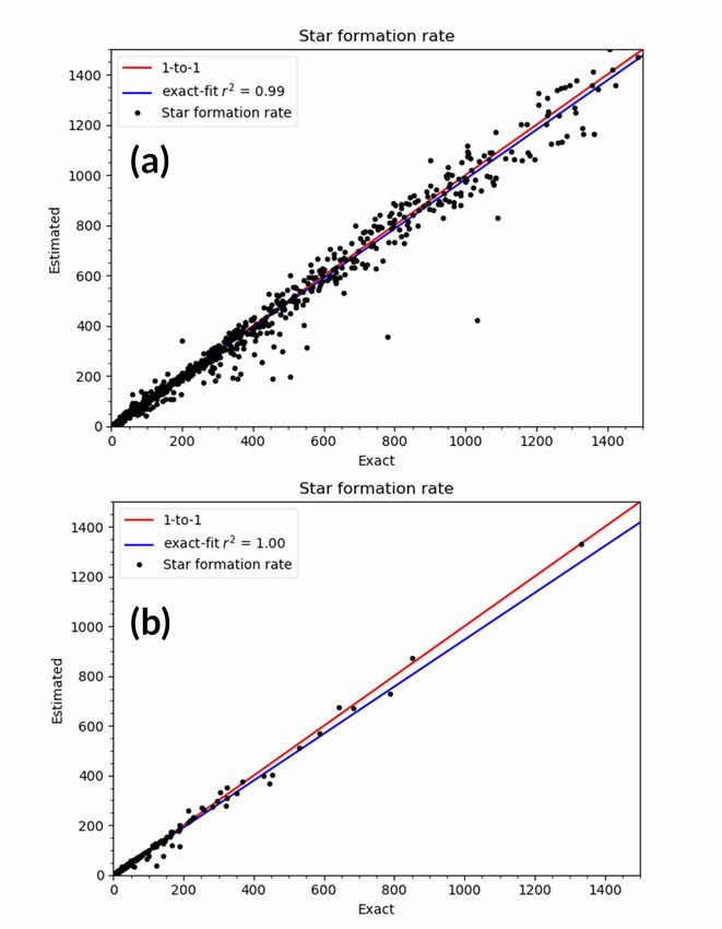
4 D. J. D. Santos et al.

Figure 1. Sample selection flowchart for this study. The left side of the flowchart summarises the MIR-FIR source selection for investigating obscuration-free
AGN activity. The right side, on the other hand, summarises the source selection in the optical wavelengths for measuring galaxy density.

tical to far-infrared (FIR) wavelengths. The multiwavelength anal- removed sources with erroneous redshift values (negative photo- 
ysis is crucial for achieving better constraint of the sources’ galaxy and/or spec- ) and deblended or saturated sources as suggested by
properties. More details about the band-merging can be read from Ho et al. (2021).
Kim et al. (2021). For CIGALE SED fitting (see Sec. 2.2), the reduced chi-square
 This work used similar selection criteria as those presented by ( 2 ) of the best-fit SED of each source must be less than 10 to
Wang et al. (2020). To summarise, in their work, the sources must be make sure that the estimated properties of the sources are reliable.
detected at the AKARI L18W band (18.0 m) and in Herschel/PACS The value of 10 was chosen as the threshold for the reduced 2
Green (100 m) or Herschel/SPIRE PSW (250 m) band to assure value as a result of our visual checks in our SED fitting results.
proper constraint of the templates used for SED fitting. The detec- In addition, it was also used by Wang et al. (2020) because of the
tion requirement in Herschel/PACS Green band or Herschel/SPIRE fact that there are at most 36 photometric points used to estimate
PSW band is implemented to make sure that there is at least one the SED of the sources and they are very likely to be correlated,
observation in the FIR region. The requirement of AKARI L18W causing the 2 value to not be well-estimated (Wang et al. 2020). We
band detection, whose bandwidth is in the longer part of the MIR also investigated the reliability of our constrained galaxy properties
band (MIR-L), is driven by its limited sensitivity compared to the (i.e., AGN contribution fraction and star formation rate) by running
other MIR bands in AKARI. To increase the sample, we also add CIGALE’s mock analysis. The results of our mock analysis is shown
another criterion which is the detection in AKARI S9W band. The in Appendix A. Our mock analysis shows that we were able to
number of detections in this band is the largest among the shorter constrain the AGN contribution fractions and star formation rates
part of the MIR bands (MIR-S). Moreover, S9W has a wide filter of our sources with enough reliability, as the estimated (mock)
width which covers the wavelength ranges of S7 and S11 bands quantities reasonably agree with the exact (true) quantities.
(Kim et al. 2012), making it a viable choice for making sure that Before the reduced 2 cut, we initially acquired 1794 all- 
at least one among the shorter and longer parts of the MIR band sources which are composed of 409 spec- sources and 1385 photo-
is available for all sources. The availability of MIR and FIR data sources. Only 119/1794 (6.6%) sources were removed with this
is important in making sure that the SED fitting is robust via the criteria, and we eventually acquired 1675 all- sources which are
energy balance principle (see Sec. 2.2 for an explanation). composed of 376 spec- sources and 1299 photo- sources. The
 The photometric redshifts (photo- ) of all the sources in the median reduced 2 of our all-z sample after the reduced chi-square
AKARI NEPW field without spectroscopic redshifts (spec- ) were cut is 3.63.
provided by Ho et al. (2021). Ho et al. (2021) performed the photo- On the right side of Fig 1, the selection criteria for constraining
 estimation with Photometric Analysis for Redshift Estimate ( the environment of our sources is shown. Density was calculated
 ℎ ; Arnouts et al. 1999; Ilbert et al. 2006), an SED template- using sources in the AKARI NEPW field detected within 5 de-
fitting code. In this study, we used spec- as the redshift values of the tection limits (with magnitude errors less than 0.2) in all bands of
sources if they were available; otherwise, we used their estimated HSC. Because it has the largest field-of-view (FoV) among optical
photo- . We selected the galaxies in our sample using the 2 value cameras on an 8m telescope (1.5 deg in diameter), HSC was able
provided by ℎ : if gal 2 < 2 (where 2 and 2 are
 star gal star to carry out an optical survey of the AKARI NEPW field with just
the minimum 2 values calculated using the galaxy and stellar 4 FoVs (Goto et al. 2017; Oi et al. 2021). The 5- detection limits
templates, respectively), the object is most likely a galaxy. We also of the HSC bands , , , , and are 28.6, 27.3, 26.7, 26.0, and

 MNRAS 000, 1–19 (2021)

Environmental Effects on AGN activity 5
25.6 (in AB mag), respectively. There are a total of ∼3 million (3M)
optically-detected sources in the AKARI NEPW field.
 As mentioned earlier, only 2026 sources have spec- , and so
the rest must rely on photo- to have their density calculated. The
photo- of the HSC-detected sources without spec- (that are not
included in the AKARI NEPW field catalog) were calculated using
 ℎ . To improve the photo- of the sources, the following data
were also added for estimating photo- : uimaging data of Canada-
France-Hawaii Telescope (CFHT; Iye & Moorwood 2003) obtained
and reduced by Huang et al. (2020), and deep Spitzer Infrared Array
Camera (IRAC) (3.6 m- and 4.5 m-band) data from Nayyeri et al.
(2018). By comparing with sources with spec- , the photo- of
the HSC-detected sources reached a photo- dispersion of 0.064
and an outlier fraction ( , defined as the number ratio of outliers
with |Δz|/(1 + )> 0.15 to the total number of sources) of 9.1%
for sources with < 1.5. Lai et al. (2016) showed that a photo- 
uncertainty of 0.06 is still acceptable for seeing the dependence
of red fraction on galaxy environment for sources at redshift ~ Figure 2. An example SED fitting result from CIGALE. The AKARI ID,
0.8. Although red fraction is not the focus of this paper, a photo- reduced chi-square, redshift, and AGN contribution fraction of the source
uncertainty of 0.064 is good enough for studying the effect of galaxy are displayed on the upper left corner.
environment on AGN activity.
 In addition, galaxy density should be calculated with galaxies
only, so star-galaxy separation was necessary. Galaxies were se-
lected based on two star-galaxy separation criteria: the HSC pipeline Wang et al. (2020). We used the delayed SFH module with op-
parameter base_ClassificationExtendedness_value (to re- tional exponential burst and parameterised age of main stellar
move extended sources), and the chi-square ( 2 ) values of the population in the galaxy. The e-folding times of the main stellar
sources using both the galaxy templates and stellar SED templates population ( main ) and the late starburst population ( burst ) were
provided by ℎ (similar to that from SED Fitting selection also fixed. In addition, we also utilised the stellar templates from
criteria). Bruzual & Charlot (2003) assuming Salpeter (1955)’s initial mass
 We would like to limit our study up to ≤ 1.2 since the photo- function. The standard default nebular emission model from Inoue
performance becomes worse at higher redshift. However, we did not (2011) was also used. The dust attenuation, on the other hand, was
want to lose sources at > 1.2 when calculating density of sources at modelled using Charlot & Fall (2000)’s attenuation law model. This
 = 1.2. At = 1.2, the redshift bin size (further discussed in Sec. 2.3) model assumes that there are two power-law attenuation curves for
is 0.14, so we restricted our density calculation up to = 1.2 + 0.14 the birth cloud and the interstellar medium (ISM) that differ on their
= 1.34. This criteria gave us 366791 sources for density calculation. default slopes. We made the slopes of these curves flexible, turning
Finally after density calculation, we have 336457 sources within z the attenuation law similar to a double power law (e.g. Lo Faro et al.
≤ 1.2 with density values. 2017; Buat et al. 2019). The V-band attenuation in the ISM ( V ISM )
 was separately parameterised but the ratio of the old stars’ V-band
 attenuation to the young stars’ V-band attenuation ( ) was fixed to
2.2 Estimation of Galaxy Physical Properties = 0.44 (Malek et al. 2018). Draine et al. (2013)’s dust emission
CIGALE1 (Boquien et al. 2019), short for Code Investigating model was utilised for our SED fitting to model the reprocessed IR
GALaxy Emission, is an SED fitting and modelling code that can dust emission absorbed from UV/optical stellar emission. Lastly, we
handle many parameters such as dust thermal emission, star for- used the AGN emission model module by Fritz et al. (2006) which
mation history (SFH), single stellar population (SSP), attenuation considers three main components using a radiative transfer model:
law, and AGN emission. We follow Wang et al. (2020)’s approach (1) the primary source of radiation located inside the torus, (2) the
in using CIGALE SED fitting to select AGNs in the AKARI NEPW dust-scattered radiation emission, and (3) the thermal dust emission
field and analyse the dependence of the sources’ AGN activity on (Boquien et al. 2019). Table 1 shows the parameter settings that we
redshift and luminosity. We used CIGALE version 2018.0 to model used in our CIGALE SED fitting. Fig. 2 shows a sample SED fitting
the optical to far-IR emission of each source. CIGALE is mainly result with CIGALE.
centred on the energy balance principle: the energy absorbed by We also used the same bands as Wang et al. (2020) for SED
dust in the UV and optical wavelengths is re-emitted in the mid- fitting. We have all 9 IR bands from AKARI/IRC (Kim et al. 2012),
and far-IR spectral regions (e.g. Burgarella et al. 2005; Noll et al. ∗ -band from CFHT/MegaCam (Hwang et al. 2007; Oi et al. 2014;
2009; Boquien et al. 2019). In this regard, it is important to have Huang et al. 2020), all 5 bands from HSC (Oi et al. 2021), , and
sufficient observations in mid- and far-IR wavelengths to accurately bands from Maidanak/Seoul National University 4K x 4K Camera
measure the absorbed and re-emitted energy. The physical mod- (SNUCAM) (Jeon et al. 2010), - and -bands from Kitt Peak
elling by CIGALE is used to fit the stellar, AGN, and SF components National Observatory (KPNO)/Florida Multi-object Imaging Near-
of each source’s SED, which enables us to get more information IR Grism Observational Spectrometer (FLAMINGOS) (Jeon et al.
about the sources’ properties. 2014), , , and bands from CFHT/Wide-field InfraRed Camera
 This work used the same modules and parameters as (WIRCam) (Oi et al. 2014), all 4 IR bands from WISE/ALLWISE
 (Jarrett et al. 2011), all 4 bands from Spitzer/IRAC (Nayyeri et al.
 2018), Green and Red bands from Herschel/PACS (Pearson et al.
1 https://CIGALE.lam.fr 2019), and all 3 FIR bands from Herschel/SPIRE Pearson et al.

MNRAS 000, 1–19 (2021)

6 D. J. D. Santos et al.

Table 1. List of modules and parameter settings for our CIGALE SED fitting.

 Parameters Value
 Delayed SFH with optional exponential burst
 e-folding time of the main stellar population [106 yr] 5000.0
 Age of the galaxy’s main stellar population [106 yr] 1000.0, 5000.0, 10000.0
 e-folding time of the late starburst population [106 yr] 20000.0
 Age of the late burst [106 yr] 20.0
 Mass fraction of the late burst population 0.00, 0.01
 Multiplicative factor controlling the amplitude of SFR if
 1.0
 normalisation is false
 SSP (Bruzual & Charlot 2003)
 Initial mass function Salpeter (1955)
 Metallicity 0.02
 Age of separation between the young and old star populations 10.0
 Dust attenuation (Charlot & Fall 2000)
 Logarithm of the V-band attenuation in the ISM -2.0, -1.7, -1.4, -1.1, -0.8, -0.5, -0.2, 0.1, 0.4, 0.7, 1.0
 Ratio of V-band attenuation from old and young stars 0.44
 Power-law slope of the attenuation in the ISM -0.9, -0.7, -0.5
 Power-law slope of the attenuation in the birth cloud -1.3, -1.0, -0.7
 Dust emission (Draine et al. 2013)
 Mass fraction of PAH 0.47, 1.77, 2.50, 5.26
 Minimum radiation field (Umin ) 0.1, 1.0, 10.0, 50.0
 dU
 Power-law slope ( dM ∝ ) 1.0, 1.5, 2.0, 2.5, 3.0
 Fraction illuminated from Umin to Umax 1.0
 AGN emission (Fritz et al. 2006)
 Ratio of the maximum and minimum torus radii 60.0
 Optical depth at 9.7 m 0.3, 6.0
 Value of in gas density gradient along the
 -0.5
 radial and polar distance coordinates (Eqn. 3 in Fritz et al. (2006))
 Value of in gas density gradient along the
 4.0
 radial and polar distance coordinates (Eqn. 3 in Fritz et al. (2006))
 Opening angle of the torus 100.0
 Angle between equatorial axis and line of sight 0.001, 60.100, 89.900
 0.0, 0.025, 0.05, 0.075, 0.1, 0.125, 0.15, 0.175, 0.2, 0.225,0.25,
 AGN contribution fraction (fracAGN ) 0.275, 0.3, 0.325, 0.35, 0.375, 0.4, 0.425, 0.45,
 0.475, 0.5, 0.525, 0.55, 0.575, 0.6, 0.625, 0.65, 0.675, 0.7

(2017). More details about their effective wavelengths, area, and Scale Environments (ORELSE) survey, and they adopted the defi-
detection limits/depth are listed in Table 2. nition fracAGN ≥ 0.1 as their AGN selection criteria. However, in
 In this work, we defined two probes of AGN activity following Wang et al. (2020)’s comparison of previously identified AGNs in
Wang et al. (2020): AGN contribution fraction and AGN number the AKARI NEPW field, they decided to select AGNs with fracAGN
fraction. AGN contribution fraction (fracAGN ) is related to the AGN ≥ 0.2 because majority of the sources with fracAGN between 0.1
luminosity in the 8-1000 m range (LAGN ) and total IR luminosity and 0.2 (69%) are not classified as AGNs in both spectroscopic and
(LTIR ): X-ray classifications. Another key result Wang et al. (2020) found
 is that AGN activity increases with redshift and not with lumi-
 LAGN = LTIR × fracAGN . (1) nosity, inferring that we may find more AGNs at higher redshift.
 On the other hand, AGN number fraction (NAGN /Ntot ) is the Using fracAGN ≥ 0.2 as our AGN selection criteria allowed us to
ratio between the number of AGNs, NAGN , and total number of select only 35/1210 AGNs. This can be attributed to our limited
galaxies, tot = NSFG+AGN within a certain bin (e.g. density, lumi- redshift range ( ≤ 1.2). Therefore, for discussion purposes, we also
nosity, redshift): adopted a less strict threshold (fracAGN ≥ 0.15) for AGN selection
 that compromises the number of selected AGNs and accuracy based
 AGN on Wang et al. (2020)’s previous comparison. In this study, we fol-
 NAGN /Ntot = (2)
 SFG+AGN lowed these two AGN selection criteria to also check whether our
 results change with varying threshold of AGN selection or not.
 Wang et al. (2020) focused on finding the relationship between
AGN activity (fracAGN and NAGN /Ntot ) and total IR luminos- Note that AGN contribution fraction and AGN number frac-
ity/redshift for MIR sources in the AKARI NEPW field. This was tion are different physical quantities. AGN contribution fraction is
made possible by using CIGALE to constrain galaxy properties and closely related to the AGN’s strength relative to its host galaxy’s
select AGNs. They compared the number of sources with varying luminosity, while AGN number fraction describes the number of
fracAGN with AGNs classified by spectroscopic surveys and Chan- AGN population with respect to a certain quantity (in this case,
dra X-ray surveys in Shim et al. (2013) and Krumpe et al. (2015), galaxy environment). One of them may exhibit different relation-
and AGNs classified using ℎ Oi et al. (2021). A similar ship with density compared to the other (Wang et al. 2020), and so
study by Shen et al. (2020) also used CIGALE to select AGNs at looking into both quantities is crucial for a better understanding of
0.55 ≤ ≤ 1.30 in the Observations of Redshift Evolution in Large AGN activity and their relationship with galaxy environment.

 MNRAS 000, 1–19 (2021)

Environmental Effects on AGN activity 7

Table 2. Summary of the 36 bands used in this study.

 Wavelength Wavelength Depth
 Band Instrument Reference
 Range ( m) (AB Mag)
 /HSC 0.47 28.6 Oi et al. (2021)
 /HSC 0.61 27.3 Oi et al. (2021)
 /HSC 0.77 26.7 Oi et al. (2021)
 /HSC 0.89 26.0 Oi et al. (2021)
 UV to /HSC 0.97 25.6 Oi et al. (2021)
 Optical ∗ CFHT/MegaCam 0.39 26, 24.6 Hwang et al. (2007); Oi et al. (2014)
 CFHT/MegaPrime 0.38 25.4 Huang et al. (2020)
 Maidanak/SNUCAM 0.44 23.4 Jeon et al. (2010)
 Maidanak/SNUCAM 0.61 23.1 Jeon et al. (2010)
 Maidanak/SNUCAM 0.85 22.3 Jeon et al. (2010)
 2 /IRC 2.3 20.9 Kim et al. (2012)
 3 /IRC 3.2 21.1 Kim et al. (2012)
 4 /IRC 4.1 21.1 Kim et al. (2012)
 7 /IRC 7.0 19.5 Kim et al. (2012)
 9 /IRC 9.0 19.3 Kim et al. (2012)
 11 /IRC 11.0 19.0 Kim et al. (2012)
 15 /IRC 15.0 18.6 Kim et al. (2012)
 Near to
 18 /IRC 18.0 18.7 Kim et al. (2012)
 Mid-IR
 24 /IRC 24.0 17.8 Kim et al. (2012)
 KPNO/FLAMINGOS 1.6 21.3 Jeon et al. (2014)
 KPNO/FLAMINGOS 1.3 21.6 Jeon et al. (2014)
 1 /ALLWISE 3.4 18.1 Jarrett et al. (2011)
 2 /ALLWISE 4.6 17.2 Jarrett et al. (2011)
 3 /ALLWISE 12.0 18.4 Jarrett et al. (2011)
 4 /ALLWISE 22.0 16.1 Jarrett et al. (2011)
 WIRCam 1.02 23.4 Oi et al. (2014)
 WIRCam 1.25 23.0 Oi et al. (2014)
 WIRCam 2.14 22.7 Oi et al. (2014)
 Near to
 IRAC1 3.6 21.8 Nayyeri et al. (2018)
 Mid-IR
 IRAC2 4.5 22.4 Nayyeri et al. (2018)
 IRAC3 5.8 16.6 Nayyeri et al. (2018)
 IRAC4 8.0 15.4 Nayyeri et al. (2018)
 PSW ℎ /SPIRE 253.7 14.0 Pearson et al. (2019)
 PMW ℎ /SPIRE 169.8 14.2 Pearson et al. (2019)
 Far-IR PLW ℎ /SPIRE 253.7 13.8 Pearson et al. (2019)
 PACS Green ℎ /SPIRE 103.7 14.7 Pearson et al. (2017)
 PACS Red ℎ /PACS 169.8 14.1 Pearson et al. (2017)

2.3 Density Estimation of each source to a certain velocity interval. The rest of the sources
 without spec- had their photo- calculated. Instead, for each source
Local density was first used by Dressler (1980) to study galaxy
 with photo- or spec- (we use spec- whenever it is available), we
morphology in clusters. It was also used by many other works due
 select neighbouring galaxies within a certain redshift bin, bin ,
to its usefulness in studying galaxy environments in groups and
 before calculating the local galaxy density. bin is calculated using:
clusters (e.g. Dressler 1980; Lewis et al. 2002) and its capability
to use redshift information of the sources to exclude foreground bin = Δ /(1+ ) (1 + ) (4)
and background sources by limiting the involved galaxy neighbours
to a specific velocity interval (Cooper et al. 2005). In addition, it where Δ /(1+ ) is the photo- dispersion of our sources for density
provides a continuous (non-discrete) measurement of environment, calculation. It is calculated using the normalised median absolute
which is advantageous compared to classifying galaxies into prede- deviation (NMAD) (Hoaglin et al. 1983):
termined environment categories (Cooper et al. 2005). In this work, p − s
we used the 10th-nearest neighbourhood method to calculate the Δ /(1+ ) = 1.48 × median (5)
 1 + s
local galaxy density of our sample (see Sec. 2.1 for the sample
selection for density calculation) which is described by Equation 3: where and are the photo- and spec- , respectively. Rearrang-
 ing this equation gives the photo- uncertainty | p − s | equal to
 10
 Σ10 = (3) bin . In addition, having the (1 + ) factor causes our redshift bins
 10 2 to be redshift dependent (i.e., increasing with redshift). The median
where 10 is the angular separation/projected distance to the 10th value of bin is 0.114, while the range of bin is 0.064 to 0.150.
nearest neighbour (measured in Mpc). As for excluding foreground One common issue in using local density as an environmental
and background sources, we are limited by the very few sources parameter is edge correction. When a target galaxy is close to the
with spectroscopic redshifts (spec- ). Only 2026 of the sources in survey edge, it is possible that there are other galaxies close to the
the AKARI NEPW field have spec- provided by Shim et al. (2013) target galaxy that is not covered by the survey. Therefore, there is a
and Miyaji et al. (2018), thereby we cannot restrict the neighbours chance that the measured density is smaller than what it is supposed

MNRAS 000, 1–19 (2021)

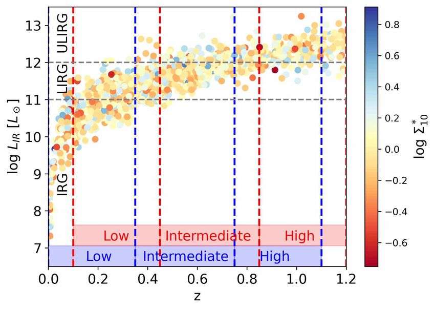
8 D. J. D. Santos et al.
to be ( is apparently "larger" because the other galaxies that may
be closer to it are outside the survey area). Previous studies (e.g.,
Miller et al. 2003) did "edge correction" by removing "edge galax-
ies" whose distances from the edge are smaller than their nth-nearest
neighbour distance. However, this edge effect may be a problem for
surveys with smaller survey areas (e.g., GOODS-North Field with
an area of 10′ × 16′ or approximately 0.044 deg2 (Giavalisco et al.
2004)) and may remove a significant number of valuable sources
for analysis (Cooper et al. 2005). Cooper et al. (2005) suggested to
recover the edge galaxies by scaling the measured counts by the
amount of aperture area covered by the survey area (this was sug-
gested under measuring galaxy environment by counting the galax-
ies within a fixed aperture size). Despite the fact that our survey
 Figure 3. A schematic diagram showing how our edge correction works.
area (5.4 deg2 ) is large enough, we would like to produce a reliable The true th nearest neighbour distance ( m ) is the th nearest neighbour
method for edge correction without removing any sources. distance ( n ). edge , on the other hand, is the distance of the source from the
 Keeping all these in mind, an edge correction method for calcu- survey edge. is the approximate fraction of the circular area (with m as
lating local galaxy density was devised and implemented to correct the radius) that is not covered by the survey. See Sec. 2.3 for a more thorough
the density of edge galaxies. A diagram explaining our method is explanation.
shown in Fig. 3. First, "edge galaxies" were selected by identifying
galaxies whose distance from the edge ( edge ) is smaller than their
 th nearest neighbour distance ( m ). Afterwards, we considered a
circular area with radius equal to the distance to m , and so this cir-
cular area must contain numbers of galaxies. We then measured
the approximate area that is not covered by the survey (that is, the
part of this circle that is outside the survey edge). Let be the ap-
proximate fraction of the area that is not covered by survey, so that
(1 − ) of the circular area contains number of galaxies. Assuming
that the number of galaxies is proportional to the area fraction (i.e.,
uniform density), we obtained the following relationship:

 = (1 − ) (6)
 Eqn. 6 tells us that the true th nearest neighbour distance
is the th nearest neighbour distance. In this method, we used the
galaxies included in the survey to estimate the edge galaxies’ "true"
local density. Our work dealt with density related to the 10th near- Figure 4. Histogram of 366791 sources with density values (top panel),
 logarithm of density, Σ10 , in Mpc−2 (middle panel, red scatterplot) and
est neighbour distance, so we set = 10. For example, if 40% of
 logarithm of normalised density, Σ∗10 , vs. redshift, . For the scatterplots,
this circular area is not covered by the survey, = 6. Therefore, the black line with 1 error bars connected in a line shows the median line.
we considered the 6th nearest neighbour as the galaxy’s "true" 10th
nearest neighbour. The robustness of this edge correction method is
more thoroughly discussed in Appendix B, where we tried different correlation coefficient of = -0.05 (both Pearson rank r-coefficient
values of aside from = 10. Our robustness tests show that among values showed a -value close to zero).
the possible values of used, = 10 performs well in terms of esti-
mating the correct local density of edge galaxies. Larger values of 
may make cluster finding algorithms using our density calculations 3 RESULTS
to be less sensitive to overdensities, while smaller values of cause
our edge correction to be erroneous. This section is dedicated to understanding the AGN activity-
 Among the 366791 HSC sources in the NEPW field with environment relation in galaxies selected in the AKARI NEPW
density values, 5601 (2%) of them are edge galaxies (with cor- field. We first discuss the distribution of our sample in terms of
rected density values). On the other hand, among the 1210 MIR-FIR luminosity and redshift in Sec. 3.1. The effect of normalised local
sources with reliable SED fits and density values at z ≤ 1.2, only density, Σ∗10 , in the AGN activity of our sources is investigated in
10 (1%) of them are edge galaxies. Despite the very low number of Sec 3.2.
edge galaxies in our sample, we believe that our edge correction is
still valuable for our research.
 3.1 Binning of MIR-FIR Sample Distribution
 The density values of each source were also normalised by the
median density of the redshift bin where it belongs to, making our In our analyses, we divided our 1210 all- sample into different
density estimator unitless. Normalisation was needed to remove the luminosity bins pertaining to different classes of infrared galaxies:
redshift dependence of density, which is shown in Fig 4. Without (normal) infrared galaxies, hereafter IRGs [log(LTIR /L ⊙ ) ≤ 11],
normalisation, the density would decrease with redshift (Pearson luminous infrared galaxies, hereafter LIRGs [11 < log(LTIR /L ⊙ ) ≤
rank correlation coefficient is = -0.37), which we attribute to faint 12], and ultraluminous infrared galaxies, hereafter ULIRGs [12 <
galaxies being less likely to be detected at higher redshifts. How- log(LTIR /L ⊙ )]. The total IR luminosity of each source were cal-
ever, normalisation alleviates this effect, producing a Pearson rank culated using Eqn. 1 by dividing the AGN luminosity by the AGN

 MNRAS 000, 1–19 (2021)

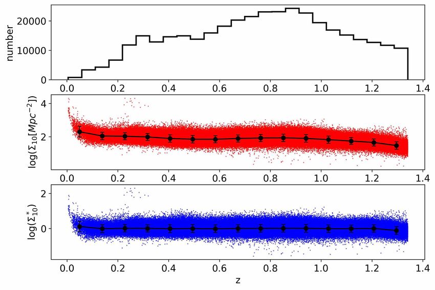
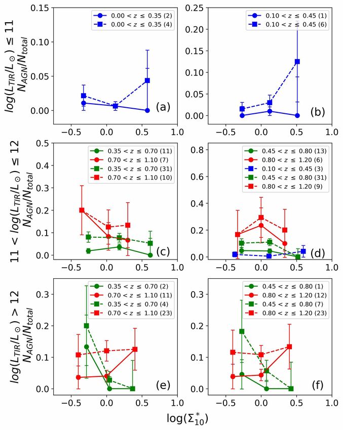
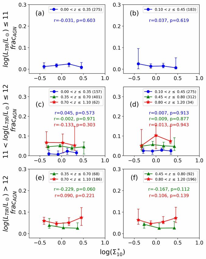
Environmental Effects on AGN activity 9

Figure 5. Scatterplot of our sources’ logarithm of total IR luminosity vs.
redshift. The redshift-luminosity bins used in this work are shown by the
dashed lines. Blue (red) dashed vertical lines show the original (shifted)
redshift bins. The gray horizontal lines show the luminosity bins. The color
of the data points refer to the logarithm of their normalised densities (log
Σ∗10 ).

contribution fraction. Then, for each luminosity bin, we further di-
vided the samples into 3 redshift bins: 0.00 < ≤ 0.35, 0.35 < ≤
0.70, and 0.70 < ≤ 1.10. However, some of the redshift-luminosity
bins had very small number of sources to produce significant statis-
tical results (sample size ≤ 10), and so they were excluded from our Figure 6. Median lines of AGN contribution fraction (frac AGN ) vs. logarithm
analyses. To include some of the removed sources in our analyses of normalised local density, log Σ∗10 , for the original redshift bins (left
and investigate how our results change with varying redshift bins, column; panels a, c, and e) and shifted redshift bins (right column; panels
we decided to shift the redshift bins by adding 0.1. The value 0.1 b, d, and f). Varying colors and markers indicate redshift bins as shown
was decided from the photo- dispersion (0.064), indicating that by the respective legends. Each row represents luminosity groups: IRG
the photo- may be uncertain by about 0.1. The resulting shifted (panels a and b), LIRG (panels c and d), and ULIRG (panels e and f). The
redshift bins were: 0.10 < ≤ 0.45, 0.45 < ≤ 0.80, and 0.80 < ≤ number of sources per redshift-luminosity bin are enclosed in parenthesis.
1.20. The reason for binning the sources is to see the dependence of For the error bars, bootstrapped (10000 times) 95% confidence intervals (for
the AGN activity-environment relation on redshift and luminosity. fracAGN ) were used. The Pearson correlation coefficients ( ) and p-values
 ( ) are also shown in each panel, following the same color coding. The
Fig. 5 shows a visualisation of our redshift-luminosity binning.
 density bins are of equal width and contain at least 15 sources (except for
 redshift-luminosity bins with < 100 sources, in which case we only make
 sure that the density bins are of equal width).
3.2 AGN Activity vs. Normalised Local Density
First, we investigated the relationship between AGN contribution
fraction fracAGN and logarithm of the normalised local density (log
Σ∗10 ) in Fig. 6. For IRGs and LIRGs, the median line of fracAGN as a
function of log Σ∗10 showed very mild to almost no trend for the first relatively lower compared to those from our IRG and LIRG samples.
two redshift bins, but the highest redshift bin (0.70 < ≤ 1.10 and However, the p-values are still large to confirm the significance of
0.80 < ≤ 1.20) for LIRGs showed large errors aside from the lack these trends. Choosing our significance level to be < 0.05 shows
of trend. As a countercheck, we also investigated the Pearson rank that the correlations between fracAGN and log Σ∗10 among different
correlation coefficients ( ) and -values of fracAGN vs. log Σ∗10 . The redshift and luminosity bins are not statistically significant.
Pearson rank correlation coefficient assesses the linear correlation We also investigated the AGN number fraction (NAGN /Ntot )
between two datasets (in this case, fracAGN and log Σ∗10 ) without as a function of log Σ∗10 in Fig 7. We first considered all sources with
taking into consideration the uncertainties from the median lines). fracAGN ≥ 0.2 as AGNs (solid lines). One limitation of this criterion
Our countercheck shows that the -values for IRGs and LIRGs are is that it selects very few sources for our analysis, contributing to
very large across all redshift bins (not to mention that their Pearson the large error bars (Poisson error) across all redshift bins for all
rank correlation coefficients are very close to zero) suggesting that luminosity groups. However, the increasing (decreasing) trend of
their correlation is not statistically significant. AGN activity (in this case, AGN number fraction) is still apparent
 However, in Fig. 6 we see for ULIRGs that at the intermediate for the highest (intermediate) redshift bin for ULIRGs. We also tried
redshift bins (0.35 < ≤ 0.70 and 0.45 < ≤ 0.80), fracAGN mildly to lower the fracAGN threshold of selecting AGNs from 0.2 to 0.15
decreases with log Σ∗10 , but this reverses at the highest redshift (dashed lines). Fig. 7 shows the result of adjusting this threshold.
bins (0.70 < ≤ 1.10 and 0.80 < ≤ 1.20). The Pearson correlation As far as the ULIRGs are concerned, the aforementioned trends are
coefficients for ULIRGs’ fracAGN vs. log Σ∗10 imply that these trends still apparent, but a larger sample of AGN further emphasised these
are small or weak (| | < 0.3). We also see that their -values are trends.

MNRAS 000, 1–19 (2021)

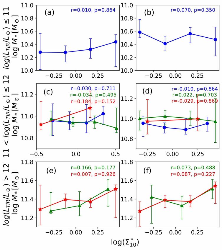
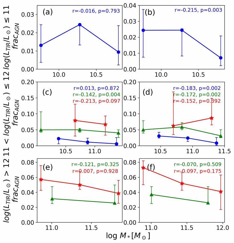
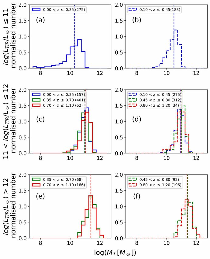
10 D. J. D. Santos et al.

 Figure 8. Histogram of log ∗ [ ⊙ ] for the original redshift bins (left col-
Figure 7. AGN number fraction (NAGN /Ntot ) vs. logarithm of normalised umn; panels a, c, and e) and shifted redshift bins (right column; panels b, d,
local density, log Σ∗10 , for the original redshift bins (left column; panels a, c, and f). Each row represents luminosity groups: IRG (panels a and b), LIRG
and e) and shifted redshift bins (right column; panels b, d, and f). Solid lines (panels c and d), and ULIRG (panels e and f). The number of sources per red-
with circle markers refer to sources with fracAGN ≥ 0.2 selected as AGNs. shift bin for each luminosity group are enclosed in parenthesis. The vertical
On the other hand, dashed lines with square markers refer to sources with dashed lines correspond to the median log ∗ [ ⊙ ] of the distributions.
fracAGN ≥ 0.15 selected as AGNs. Varying colors indicate redshift bins as
shown by the respective legends. Each row represents luminosity groups:
IRG (panels a and b), LIRG (panels c and d), and ULIRG (panels e and
f). The number of sources per redshift bin for each luminosity group are shift bin (0.00 < ≤ 0.35). For the shifted redshift bins, the LIRGs
enclosed in parenthesis. For the error bars, Poisson error bars were used. at the lowest (0.10 < ≤ 0.45) and intermediate (0.45 < ≤ 0.80)
The density bins are of equal width and contain at least 15 sources (except shifted redshift bins showed significant difference ( ≈ 0.003). The
for redshift-luminosity bins with < 100 sources, in which case we only make rest have very high -values ( ≥ 0.23). However, our ULIRGs’
sure that the density bins are of equal width). For NAGN /Ntot = 0, Poisson did not show any significant differences in their stellar mass dis-
single-sided upper limits corresponding to 1 (Gehrels 1986) are shown. tributions even at the shifted redshift bins ( ≥ 0.29). The mixed
 results of significant differences in the stellar mass distributions of
 our LIRGs may have caused the absence of apparent correlation
4 DISCUSSION between AGN activity and environment. However, for ULIRGs, the
 effect of stellar mass is not so strong or has no clear evidence of
4.1 Effect of Stellar Mass
 affecting our results.
In this section, we discuss the effect of stellar mass on our re- We also investigated the relationship between stellar mass
sults, especially in the suggested reversal trend observed in the and density/AGN activity. Previous studies (Elbaz et al. 2007;
SFR-density relation for our ULIRG sample. Since our results sug- Hwang, Shin, & Song 2019) showed a reversal in SFR-density re-
gest a reversal in the relationship between AGN activity and en- lation at higher redshifts (increasing SFR with increasing density
vironment in ULIRGs, we need to check the stellar mass distri- in contrast with lower redshifts). They explored the effect of stellar
butions of our sources at different redshift-luminosity bins. Fig 8 mass in their observed reversal trend. In Elbaz et al. (2007)’s work,
shows the histogram of the sources’ logarithm of stellar mass, log if SFR increases with stellar mass at higher redshifts and stellar mass
 ∗ [ ⊙ ]. As expected, increasing luminosity implies increasing increases with density at higher redshifts, stellar mass may serve
stellar mass distributions. For each luminosity group, we also per- as a physical reason why there is enhanced SF activity in denser
formed a Kolmogorov-Smirnov (KS) test as a countercheck. For environments at higher redshifts. In our work, instead of looking
LIRGs, we found relatively significant differences for pairs of stel- at SFR, we explore the correlation between fracAGN and log ∗ ,
lar mass distributions. For instance, we have ≈ 0.018 for the stellar and stellar mass and log Σ∗10 . These are shown in Figs. 9 and 10,
mass distributions of LIRGs in the highest original redshift bin (0.70 respectively. Although our small sample size limits us to reach high
< ≤ 1.10) and the intermediate original redshift bin (0.35 < ≤ significance levels ( < 0.05) in most of our redshift-luminosity
0.70). We also have ≈ 0.063 for the stellar mass distributions of bins, it is quite clear that just by looking at our ULIRG sample,
LIRGs in the highest original redshift bin and lowest original red- their fracAGN decreases with stellar mass (which is also suggested

 MNRAS 000, 1–19 (2021)

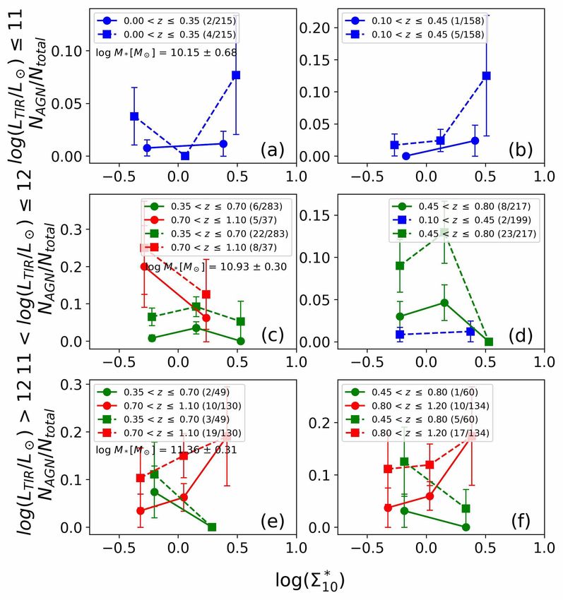
Environmental Effects on AGN activity 11

Figure 9. Similar to Fig. 6, but for fracAGN vs. log ∗ [ ⊙ ]. The same
legends apply.
 Figure 10. Similar to Fig. 6, but for log ∗ [ ⊙ ] vs. log Σ∗10 . The same
 legends apply.
in the other luminosity bins), and stellar mass increases with log Σ∗10
(which is less marginal in other luminosity bins) across intermedi-
ate and high redshift bins, regardless of shifting them or not. This
implies that we should expect that fracAGN decreases with log Σ∗10
across all redshift bins as far as our ULIRG sample is concerned.
However, this is not what our results show (panels (e) and (f) in Fig.
6), as we see that fracAGN increases with Σ∗10 at our highest redshift
bin. Our results suggest that there is a possibility of environmental
dependence of AGN activities in ULIRGs.
 Hwang, Shin, & Song (2019), on the other hand, looked at the
possibility of the observed SFR-density reversal being an effect of
galaxies in different density bins having different stellar masses. To
verify this, they narrowed the mass range of the sample galaxies
and tried to observe the same reversal trend. We implored the same
method in Fig. 11, wherein we narrowed down the mass range
of our luminosity bins by selecting galaxies within the average
log ∗ [ ⊙ ] ± the standard deviation of log ∗ [ ⊙ ] for each
luminosity bin. It is clear from Fig. 11 that even if restrict our
sample into narrow stellar mass bins, the reversal in AGN number
fraction-environment relation for ULIRG remains unchanged. We
therefore conclude that stellar mass does not have a strong effect in
the suggested reversal trend in ULIRG AGN activity-environment.

4.2 Selection bias due to FIR detection
The FIR detection, as also explained by Wang et al. (2020), also
 Figure 11. Similar to Fig. 7, but for each luminosity bin (each row), the
produces selection bias for our study. As explained earlier, this cri-
 stellar mass of the sample are narrowed down (the stellar mass ranges for
terion is important to make sure that our SED fitting is robust via each luminosity bin are shown in the first column). In the legends of each
the energy balance principle. The resulting selection bias happens panel, the number of AGNs over the new total number of sources per redshift-
because this criterion will make the sources flux-limited in FIR at luminosity bins are shown. The same legends apply.
higher redshift. This also means that we can only select very lumi-
nous FIR galaxies at high redshift, and high- objects dominated
by AGNs but lack far-IR detection might be dropped from our sam-
ple due to this criteria. We therefore expect that majority of our
galaxies have high star-formation activity. However, because of the

MNRAS 000, 1–19 (2021)